

Abstract
We have used an analysis of signal and variation in motor behavior to elucidate the organization of the cerebellar and brain stem circuits that control smooth pursuit eye movements. We recorded from the abducens nucleus and identified floccular target neurons (FTNs) and other, non-FTN vestibular neurons. First, we assessed neuron-behavior correlations, defined as the trial-by-trial correlation between the variation in neural firing and eye movement, in brain stem neurons. In agreement with prior data from the cerebellum, neuron-behavior correlations during pursuit initiation were large in all neurons. Second, we asked whether movement variation arises upstream from, in parallel to, or downstream from a given site of recording. We developed a model that highlighted two measures: the ratio of the SDs of neural firing rate and eye movement (“SDratio”) and the neuron-behavior correlation. The relationship between these measures defines possible sources of variation. During pursuit initiation, SDratio was approximately equal to neuron-behavior correlation, meaning that the source of signal and variation is upstream from the brain stem. During steady-state pursuit, neuron-behavior correlation became somewhat smaller than SDratio for FTNs, meaning that some variation may arise downstream in the brain stem. The data contradicted the model's predictions for sources of variation in pathways that run parallel to the site of recording. Because signal and noise are tightly linked in motor control, we take the source of variation as a proxy for the source of signal, leading us to conclude that the brain controls movement synergies rather than single muscles for eye movements.
Keywords: brain stem, electrophysiology, motor noise, motor synergies, variability
our goal is to ask whether the brain generates conjugate eye movements by controlling synergies or single muscles [e.g., Evarts (1968); Overduin et al. (2012); Todorov (2000)]. Our approach is based on an earlier, simplified analysis in the cerebellar cortex of the relation between neural and motor variation (Medina and Lisberger 2007). These authors showed that shared variation across the population of floccular Purkinje cells leads to an impressive trial-by-trial correlation between the firing rate of the Purkinje cells and the ensuing eye movements. Further analyses have revealed the same “neuron-behavior” correlation in extrastriate visual area middle temporal (MT) (Hohl et al. 2013) and in the smooth eye-movement region of the frontal eye fields (Schoppik et al. 2008). In the present study, we have again studied neuron-behavior correlations but used a more general model with the broader goal of understanding the organization of the oculomotor circuits in the brain stem.
Signal and variation are linked in sensory-motor circuits in the sense that the size of the noise depends on the size of the signal (Harris and Wolpert 1998; Medina and Lisberger 2007). This link suggests a common source for signal and noise in motor control. As a result, discovery of whether variation is distributed to movement synergies or to single muscles would serve as a proxy for the same question about signal. If we found evidence that variation in the movement command is distributed uniformly to all pathways in the downstream motor circuits, then we could conclude that motor commands specify high-level parameters of the movements and drive synergies rather than single muscles. For example, horizontal eye movements are generated by the lateral and medial rectus muscles, which are innervated by motoneurons in the abducens and oculomotor nuclei. If the brain controls synergies, then we would find evidence of correlated variation in the activity of the two motoneuron populations. If the brain controls muscles separately, then we would find evidence that variations in the firing of abducens and oculomotor neurons are uncorrelated to some degree. The distinction between higher control of movement synergies and single muscles has not been of great concern in eye movements [but see also Zhou and King (1998)]. Still, eye movements have the advantage of allowing clean, quantitative assessment of general questions, possibly leading to future applications to the more complex problem of controlling somatic movements.
For the system we study, smooth pursuit eye movements, the specifics of the essential circuit (Lisberger 2010) suggest a general framework for thinking about the sources of motor variation. From the perspective of any given recording site, the source of motor variation could be upstream from that site, downstream from that site, or in a pathway that runs in parallel to that site. For example, relative to the motoneurons in the abducens nucleus, motor variation could arise: upstream in a source that provides equal inputs to the medial and lateral rectus motoneurons; independently in parallel in the pathways to the agonist and antagonist lateral and medial rectus motoneurons; or downstream in the motor periphery.
Our strategy was to test the data against the predictions of a model that extends the prior analysis in the cerebellar flocculus (Medina and Lisberger 2007). The model developed a theoretical/computational framework that allows us to infer what we want to know [the sources of motor variation (and signal)] from what we can measure (the neuron-behavior correlations and firing-rate variance of identified brain stem neurons). Our analysis of these two parameters for neurons in the abducens nucleus and nearby regions of the brain stem implies that all of the variation in the initiation of pursuit arises upstream from the brain stem and is “shared” uniformly by the different parallel pathways in the brain stem. During steady-state tracking, some variation may arise in the circuits between neurons that receive monosynaptic inhibition from the cerebellar flocculus (FTNs) and motoneurons. Because variation and signal arise together, we conclude that the pursuit motor system controls movement synergies rather than single muscles. Signals for the initiation of pursuit and steady-state tracking are distributed uniformly to the parallel neural pathways that create the final motor commands.
MATERIALS AND METHODS
Data were collected from two male rhesus macaque monkeys (Macaca mulatta) that had been prepared for electrical stimulation, behavior, and neural recording using techniques described in detail previously (Joshua et al. 2013). All procedures had been approved in advance by the Institutional Animal Care and Use Committee at the University of California, San Francisco, where the experiments were performed. Procedures were in strict compliance with the National Institutes of Health Guide for the Care and Use of Laboratory Animals.
Briefly, we implanted hardware to allow us to restrain the monkey's head and a coil of wire on one eye (Ramachandran and Lisberger 2005) to measure eye position, using the magnetic search coil technique (Fuchs and Robinson 1966). After they had recovered from surgery, we trained the monkeys to track spots of light that moved across a video monitor placed in front of them. In a later surgery, we used a trephine to make a hole in the skull, and we implanted a recording cylinder aimed at the brain stem (Lisberger et al. 1994). Glass-coated, platinum-iridium electrodes were then lowered into the brain stem to record from neurons in the vestibular and abducens nuclei. To identify neurons that received monosynaptic inhibition from the floccular complex of the cerebellum, we implanted a bipolar-stimulating electrode (Rhodes Medical Instrument, Woodland Hills, CA) chronically at a site in the floccular complex where stimulation with single pulses or brief trains caused smooth eye velocity toward the side of stimulation, with a latency of ∼10 ms (Lisberger et al. 1994).
Experimental design.
Visual stimuli appeared on a Barco monitor at a distance of 30 cm from the monkey's eye. Targets were bright, 0.6° circles on a dark background. All experiments were carried out in a dimly lit room. To classify each neuron, we characterized its responses under several different tracking conditions. To determine the relationship between neuronal firing rate and eye position, the target moved in 5° steps to a variety of different positions over a range of ±20°, while the monkeys fixated within a 3° square window for an interval of 1 s or 1.5 s. To determine the relationship between neuronal firing rate and smooth pursuit with the head stationary, we provided sinusoidal target motion along the horizontal or vertical axis. To determine the contribution of vestibular inputs, the target either moved exactly with the monkey during sinusoidal vestibular rotation [vestibuloocular reflex (VOR) cancellation] or remained stationary in space during the same rotation (VOR in the light). Sinusoidal stimuli were at 0.5 Hz ± 10°.
After classifying each neuron, we recorded its responses during pursuit of step-ramp target motions (Rashbass 1961), presented in discrete trials. At the start of each trial, a stationary target appeared, and monkeys were required to fixate within a 2–3° square window for an interval that was randomized between 500 and 700 ms. The target then displaced to a location eccentric to the position of gaze (step) and immediately began moving toward the fixation point (ramp). The size of the displacement was chosen to minimize the presence of initial saccades and hence, varied slightly between monkeys, recording days and target speeds. Neurons were tested in several pursuit conditions. To compare responses with different directions of movement, the target ramp had a speed at 30°/s and moved in the on or off direction of the neuron under study. In experiments that varied the initial eye position, the movement started at the center of the screen or at an offset of 10° in the off direction of the neuron under study and then underwent a step-ramp motion, with the ramp in the on direction at 30°/s. In some experiments, in monkey I, we presented step-ramp target motion in the on direction of the neuron under study at 30°/s or 10°/s, usually starting from a fixation position that was offset 10° toward the off direction of the neuron.
Neural database.
We recorded from 112 abducens neurons (44 and 68 from monkeys I and P) and 243 neurons in the region of the vestibular nucleus (206 and 37 from monkeys I and P). For the analysis of neuron-behavior correlations, we used cells that were well isolated for more than 30 trials of pursuit: 52 abducens neurons and 131 vestibular neurons passed these criteria. Of the 131 vestibular neurons, 30 were identified as FTNs, because they were inhibited at monosynaptic latencies by stimulation in the floccular complex. An additional five neurons were excited by floccular stimulation. Of the vestibular neurons that were not inhibited or excited by floccular stimulation, 37 responded to eye and head movement in the same direction during pursuit with the head stationary and cancellation of the VOR and were classified as “eye-head velocity” (EHV) neurons. Twenty-seven neurons responded to eye and head motion in the opposite direction during pursuit with the head stationary and cancellation of the VOR and were classified as “position-vestibular-pause” (PVP) neurons. Twenty-two neurons responded only to eye movement and were classified as “eye-movement” neurons. The remaining 10 neurons did not fall in any of these categories or could not be categorized because of too little data. The five neurons that were excited orthodromically by stimulation in the floccular complex were grouped with FTNs, because they had similar response properties. We did not study neurons that lacked response modulation during smooth eye movements with the head stationary, leading us to exclude the “vestibular-only” neurons.
Of course, neurons still could have been FTNs, even if they were not inhibited at monosynaptic latencies by stimulation through the electrodes that we implanted in the floccular complex. For example, it is possible that there are differential projections from different parts of the larger floccular complex that comprise the flocculus and the ventral paraflocculus. The most likely candidates for this class of error would be the EHV neurons, which have many but not all of the response properties of neurons that we identified as FTNs (Joshua et al. 2013). Therefore, we reanalyzed our data after grouping the EHV neurons with the FTNs, but we did not find any changes that affected our conclusions. We cannot provide histological verification of the location of the stimulating electrodes, because the monkeys have been explanted and donated to a sanctuary. However, we think that the locations of the electrodes are similar to what we have reported before (Lisberger et al. 1994), because of the similar eye movements evoked from the electrodes and the similar response properties of the neurons identified as FTNs.
Data acquisition and analysis.
To measure and quantify eye movements, we scaled the signals from the eye coil monitor to obtain signals related to horizontal and vertical eye position. We then passed the position voltages through an analog circuit to create signals proportional to horizontal and vertical eye velocity. The circuit differentiated frequency content from 0 to 25 Hz and filtered higher frequencies with a rolloff of 20 dB/decade. Signals related to eye position, eye velocity, and turntable angular velocity were digitized at 1,000 samples/s on each channel. We calculated eye acceleration by differentiating the velocity signals. We used the reciprocal of the interspike interval to convert the spike train for each individual pursuit trial to a continuous firing-rate variable. We then filtered eye position, velocity, acceleration, and firing rate using a low-pass digital filter with a cutoff at 12.5 Hz and a rolloff of 20 dB/decade. The application of filters with cutoffs at higher frequencies made our data noisier but did not alter any of our conclusions. Saccades were replaced with straight-line segments before filtering. After filtering, neural data and eye movements from 40 ms before to 40 ms after the saccade were treated as missing data. The use of step-ramp target motions caused catch-up saccades to have fairly long latencies, and we were able to obtain enough repetitions to perform our analysis, even though we omitted from analysis any spike trains that had bursts or pauses related to saccades in the analysis interval.
Model with shared and parallel noise.
The goal of our computational model is to compare the predictions of various circuit configurations with the data measured in the experiments. The three quantities that we measured in the experiment are the trial-by-trial correlations between neural and behavior variations, the trial-by-trial variation in firing rate, and the trial-by-trial variation in eye movement. In the following section, we develop the equations that will allow us to compare the data with the model.
We assume the variation in the firing rate of a neuron has three components
| (1) |
where ηup represents “upstream” variation that is shared across all neurons in the network, ηparallel represents variation that is restricted to one of two parallel populations of neurons, and ηind represents variation that is independent in each neuron. In the term fri,j, j can be one or two and represents two parallel groups of model neurons, whereas i ranges from one to n and indexes the model neurons within each population. Among the sources of variation, ηup lacks an index, because it is distributed to all model neurons in both parallel populations; ηjparallel is indexed only by j, because there are separate sources of variation for each of the two parallel populations; and ηi,jind is indexed by i and j, because it is drawn independently for each model neuron.
To contrive the variances of each quantity to have the proper relation to the variance of firing rate, we define
| (2a) |
| (2b) |
| (2c) |
Here, Vx is a scalar gain that describes the fractional contributions of source “x” to the variance of firing rate. We assume that the three sources of variation are independent so that their covariance terms are zero in the equations that follow.
The eye movement is derived from the population activity in the network and is defined as
| (3) |
where N1 and N2 are the number of active neurons in the two parallel groups of model neurons, and ηdownstream is an additional source of variation (variance = σDS2) that is added to the eye-movement command after pooling of the responses of the two groups of model neurons. The downstream variation is independent of all other sources of variation, so that covariance (cov)(ηdownstream,fri,j) = 0. Equation 3 defines a linear relationship between eye movement and firing rate in the model, normalized by the number of neurons in the model. This is different only in detail from the situation in the data, where we created a linear relationship by using regression on eye kinematics to transform eye movement into the units of firing rate (see Eq. 12 below).
To be able to compute the trial-by-trial correlation between the firing rate of each model neuron and the output of the model (“Eye” in Eq. 3), we use the definitions in Eqs. 1–3 to formulate equations for the variance of firing rate and eye movement
| (4) |
| (5a) |
We can substitute Eq. 4 into Eq. 5a, because by definition, the different sources of variation are independent, and the covariance terms are zero
| (5b) |
By substituting the variance terms with the right sides of Eq. 2, a–c, we obtain
| (5c) |
The presence of a large number of neurons means that the independent noise disappears through averaging, yielding
| (5d) |
To simplify the equations, we define Gi as the fraction of active neurons in group i relative to the total number of active neurons, Gi ≡ Ni/(N1 + N2), yielding
| (6) |
The ratio between the SDs of the network output and the firing rate of the neurons will turn out in results to be important for analyzing the sources of variation. Therefore, we have termed the ratio of the SDs of neural firing rate and eye movement (SDratio), and we have computed it as
| (7) |
To calculate the neuron-behavior correlation, we develop the term for the covariance between the firing rate of a model neuron and the eye movement
| (8) |
To expand and then simplify this equation, we assume j = 1, so that the neuron is part of group 1, and all covariance terms with parallel variation from group 2 are equal to zero. In addition, all of the terms that contain different, independent sources of variation are, by definition, equal to zero. Finally, the independent noise is small compared with the number of neurons. This allows us to simplify and derive the equations for neuron-behavior correlation
| (9) |
To derive the equation for neuron-behavior correlation, we use the equations developed for the covariance in Eq. 9 and for the variance of firing rate and eye movement in Eqs. 4 and 6:
| (10a) |
| (10b) |
| (11) |
In results, we use Eqs. 7 and 11 to compare model predictions with the neuron-behavior correlation (RNB) and the SDratio in our data.
RESULTS
Our presentation will unfold in three steps. First, we verify the expectation from our prior study that we will find impressive trial-by-trial correlations between the firing rate of brain stem neurons and pursuit eye movements, i.e., RNB. Although we expect this conclusion, it need not be so. In principle, correlation coefficients could take any value between -1 and 1 and could modulate dynamically as a function of time. Indeed, the exact value and temporal modulation of RNB are critical pieces of information for our larger goal of specifying how signals are processed in the brain stem premotor circuits for eye movements. Second, we develop and explore a general model of circuit organization and use it to understand the implications of different sources of neural signal and variation for the organization of the motor command. Third, we use the predictions of our general model to guide the analysis of our data. We make the link from measures of RNB to what we want to know, namely whether motor commands for eye movement are distributed to movement synergies or independently to individual muscles.
Correlation between neural activity and behavior during smooth pursuit.
The goal of this section is to demonstrate the existence of RNB in the various brain stem neurons that we are able to identify, determine the magnitude of the correlations, and characterize how the correlations evolve through a full pursuit eye movement. The resulting description will provide the database for advancing our understanding of the organization of the final motor pathways in the rest of the paper.
We recorded neural and behavioral responses, as monkeys moved their eyes to track a target that was stationary initially and then moved at constant speed on a display in front of them. As shown in Fig. 1A, the monkey's eye began to rotate smoothly after a short delay of ∼100 ms from the onset of step-ramp target motion (Rashbass 1961). Later in the trial, eye velocity reached and remained similar to target velocity, almost until the target stopped moving. The choice of the correct amplitude for the target step obviated the need for a saccade during movement initiation, creating eye position records that are largely free of saccades. Eye acceleration shows a positive pulse at the start of the pursuit response and a negative pulse at the end. Across multiple repetitions of the same target motion, individual eye-movement responses (Fig. 1A, gray traces) showed some trial-to-trial variation but grouped fairly tightly around the average responses (black traces).
Fig. 1.
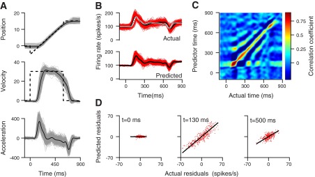
Neuron-behavior correlation (RNB) between firing rate and eye movement for an example floccular target neuron (FTN). A: for eye kinematics, gray traces illustrate single trials, and solid black traces show the average across all trials. B: The 2 sets of traces show actual and predicted firing rate for a FTN neuron. Black and red lines show the averages across trials and many single-trial responses. C: the RNB matrix. The color of each pixel indicates the strength of the trial-by-trial correlation between predicted firing rate at the time on the vertical axis and the actual firing rate at the time on the horizontal axis. D: trial-by-trial correlation between actual and predicted firing rate at 3 separate times: fixation (t = 0 ms), initiation (t = 130 ms), and steady-state pursuit (t = 500 ms). Each point shows data from a different trial. The black lines show the results of linear regression.
We identified the various brain stem neurons according to criteria detailed in a prior paper (Joshua et al. 2013). Abducens neurons had a characteristic, very regular firing in relation to eye movement and were located in a group of “singing” neurons, with the well-known response properties of motoneurons (Fuchs and Luschei 1970). FTNs showed a full cessation of spontaneous activity at monosynaptic latencies after application of a single shock through an electrode implanted in the floccular complex of the cerebellum. Other, non-FTN vestibular neurons did not show any sign of inhibition after stimulation in the floccular complex and included traditional PVP neurons, as well as other neurons that showed modulation of firing rate in relation to eye movement and/or passive vestibular rotation. The response properties of FTNs and non-FTNs in the present sample agreed well with those in prior studies of the same area of the brain stem (Lisberger et al. 1994; Ramachandran and Lisberger 2008).
To study the trial-by-trial relationship between the variations in the behavior and the firing of single neurons in the pursuit motor pathways, we used the approach described by Medina and Lisberger (2007). Because the average firing rate of brain stem neurons is described well by a simple linear regression model (Joshua et al. 2013), we fitted the average response of each cell to a linear weighted sum of the average eye kinematic parameters (E, position; Ė, velocity; and Ë, acceleration) (Fuchs et al. 1988; Medina and Lisberger 2007; Scudder and Fuchs 1992; Sylvestre and Cullen 1999)
| (12) |
where rr is firing rate during fixation toward the midline, and Δt indicates by how much time the eye-movement averages need to be shifted to optimize the fit to the average firing rate. The values of parameters a, r, and k represent the sensitivity of a cell to eye acceleration, velocity, and position. We used the parameters that provide the best fit to the responses for all target speeds and initial eye positions in a given direction, and we also confirmed that the parameters were very similar when Eq. 12 was fitted to the average responses for each individual target motion. We did not separate the trial-to-trial variation into components related to the latency vs. speed of pursuit (Osborne et al. 2005). The mean latencies of pursuit were 86 ms and 87 ms, and the SDs of 8.3 ms and 11.4 ms were small enough in the two monkeys so that latency variation would have little impact on our findings.
We used the regression model for the mean responses to transform the eye movement in each behavioral trial into a surrogate in units of spikes/s, allowing us to use the same units to correlate eye movement with firing rate and assess the extent to which they co-vary. This approach is better than correlating actual firing rate with eye acceleration, velocity, or position, because it takes into account all of the parameters of eye movement that affect a neuron's firing rate. For the FTN, illustrated in Fig. 1B, and all other neurons (Joshua et al. 2013), the approach, based on the regression equation, is validated by the good agreement between the average of actual firing rate and the predictions based on the average eye movements (compare black and white traces in the top of Fig. 1B or the “actual” and “predicted” traces in the same panel).
The FTN, illustrated in Fig. 1, showed a strong correlation between the trial-by-trial variations in firing rate and eye movement at the initiation of pursuit. In Fig. 1C, the color of each pixel indicates the correlation coefficient for actual vs. predicted firing rate at the times indicated by the location of the pixel on the horizontal and vertical axes. The largest correlations occurred along the diagonal for pixels that represent correlations with zero or small time lags between actual and predicted firing rate (defined by Δt in Eq. 12). The larger blob of redder pixels along the diagonal close to the bottom left of the image indicates larger correlations at movement initiation. For this particular FTN, the correlation coefficient reached a maximum of 0.88 at 130 ms after the onset of target motion. Correlations were strongest along the entire diagonal of the matrix but in general, had lower values (yellow pixels) during steady-state pursuit, starting ∼200 ms after the onset of target motion. Correlations were very weak (blue pixels) before the onset of pursuit, at times before 100 ms. Weak oscillations in steady-state eye velocity during pursuit led to the periodic bands that run parallel to the diagonal.
For brain stem neurons, the RNB was very clear in scatter plots from individual times during pursuit. In the examples shown in Fig. 1D, we calculated the residuals of the actual and predicted firing rate in each trial by computing the absolute (predicted or actual) firing rate minus the mean (predicted or actual) firing rate as a function of time. We then plotted the residuals from each trial as a separate symbol. The results show a very low correlation at time 0 (r = 0.05); a high correlation, 130 ms after the onset of target motion (r = 0.88); and an intermediate correlation, 500 ms after the onset of target motion (r = 0.56).
FTNs, non-FTN vestibular neurons, and abducens neurons displayed patterns of RNB that were qualitatively similar but quantitatively different. The images in Fig. 2, A–C, show the averages of the full correlation matrices across all recordings from each population. In all three populations, the average RNB was small at fixation, peaked at movement initiation, and continued at lower levels along the diagonals throughout steady-state pursuit. The FTNs (Fig. 2A) had a large RNB close to the initiation of pursuit, as illustrated by the red pixels at times between 100 and 200 ms after the onset of target motion. During steady-state pursuit, FTNs showed smaller values of RNB, illustrated by the light blue colors along the diagonal of the matrix in Fig. 2A. Non-FTN vestibular neurons (Fig. 2B) showed the same general pattern as FTNs, with lower values of RNB during steady-state pursuit vs. pursuit initiation. However, the values of RNB were lower throughout the movement in non-FTN vestibular neurons vs. FTNs. Abducens neurons (Fig. 2C) showed very high values of RNB throughout the pursuit behavior but still with somewhat larger values during pursuit initiation vs. steady-state pursuit. The wider swath of high correlations along the diagonal for abducens neurons vs. FTNs can be attributed to the sensitivity of abducens neurons to eye position and the resulting correlations across time in each behavioral trial.
Fig. 2.

Population averages of RNB. A–C: the color of each pixel indicates the strength of the trial-by-trial correlation between predicted firing rate at the time on the vertical axis and the actual firing rate at the time on the horizontal axis for FTNs (A), non-FTN vestibular neurons (B), and abducens neurons (C). D and E: the continuous traces show the value of RNB along the diagonals of the images in A–C as a function of time from the onset of target motion. The shading around the traces shows the SE across neurons. Different colored traces show results for different groups of brain stem neurons, and the black line shows the results for floccular Purkinje cells from Medina and Lisberger (2007). E only, modulation during eye movement with the head stationary but not during cancellation of the vestibuloocular reflex; PVP, position-vestibular-pause; EHV, eye-head velocity.
To quantify the patterns of RNB in the different populations of neurons, we measured the values of RNB along the diagonal of the correlation matrix as a function of time from the onset of target motion for each neuron. We then averaged the curves relating RNB to time for all neurons within each sample population and superimposed them in Fig. 2D for direct comparison. In the 100 ms before the onset of target motion, the large eye position sensitivity of abducens neurons and the small fluctuations of fixation position led to values of RNB larger than those of FTNs and vestibular neurons (0.19 vs. 0.07 and 0.08; P < 0.001 one-way ANOVA; Tukey's post hoc comparison). During the initiation of pursuit, the RNB of abducens neurons (blue traces) and FTNs (red traces) reached identical peak values of 0.65, but the FTNs reached a sharper peak at a slightly earlier time (130 ms vs. 190 ms after the onset of target motion). The peak RNB of the non-FTN vestibular neurons was significantly lower compared with the other populations (RNB = 0.31; P < 0.001 one-way ANOVA; Tukey's post hoc comparison). During steady-state pursuit, 500 ms after the onset of target motion, RNB was largest for abducens neurons, moderate for FTNs, and smallest for non-FTN vestibular neurons (RNB = 0.5, 0.31, and 0.16; P < 0.001 one-way ANOVA; Tukey's post hoc comparison).
To compare RNB across more of the pursuit circuit, we also plotted RNB as a function of time for a population of Purkinje cells recorded in the cerebellar floccular complex by Medina and Lisberger (2007), during very similar eye-movement behavior. The peak values of RNB during the initiation of pursuit were similar in FTNs (red trace) and Purkinje cells (black trace), whereas the steady-state values of RNB were somewhat larger for FTNs. Note that the black trace for Purkinje cells in Fig. 2D stays high for a longer time than do the colored traces for brain stem neurons, because the pursuit trials were 100 ms longer in the recordings of Medina and Lisberger (2007) than in our experiments.
Finally, we divided the non-FTN vestibular neurons into smaller groups, according to their functional response properties in relation to eye movement and vestibular rotation (Fig. 2E). Compared with the values in FTNs (red trace), RNB was relatively small in all groups. The smallest correlations occurred in neurons that discharged in relation to eye position and velocity in one direction, with the head stationary and head velocity in the opposite direction during cancellation of the VOR (“PVP”; P < 0.05 one-way ANOVA on the peak of the RNB in the first 300 ms after target motion; Tukey's post hoc comparison). RNB were intermediate in the neurons that showed modulation during eye movement with the head stationary but not during cancellation of the VOR (“E only”) and for the EHV neurons. EHV neurons were not inhibited by stimulation through the electrodes in the floccular complex but like FTNs, showed modulation during eye and head motion in the same direction for recordings with the head stationary and during cancellation of the VOR. We cannot exclude the possibility that the EHV neurons might have been classified as FTNs if the stimulating electrodes had been placed elsewhere within the floccular complex.
The sources of motor variation.
In the present section, we move forward from the description of the time course of RNB to analyze the sources of variation for each neuron and for the motor output. Specifically, we ask the extent to which neural variation arises from a shared correlation with the evoked movement across the population vs. independent variability that could arise from the intrinsic noise in spike generation. We also ask whether it is necessary to postulate noise added downstream from each neuron population to account for the variation in eye movement.
We start with simple algebra to show how we can estimate each component of the variation independently. After Medina and Lisberger (2007)
| (13a) |
where RNB is the neuron-behavior correlation for a particular neuron, σEye2 is the variance in eye movement, σFR and σEye are the SDs of firing rate and eye movement, and σDS2 is the variance in motor output that is generated downstream from the neuron under study. Intuitively, the variation in the eye movement is divided into two components. The first component is shared across all neurons in a given population. Because shared variation is not reduced through averaging across neurons, it leads to RNB. The first term on the right side of Eq. 13a represents the contribution of shared variation to eye movement and is equal to the covariance of the firing rate and the eye movement. The second component of eye-movement variation comes from variation that is added downstream from the neurons under study. It is represented by the second term on the right side of Eq. 13a. Simple algebra converts Eq. 13a into Eq. 13b and shows how we can estimate the downstream noise from what we can measure—eye-movement variance, firing-rate variance, and RNB
| (13b) |
We can compute the variation that is shared across the population, and probably arises upstream from the recording site, as the difference between the overall variation in eye movement and the variation that originates downstream
| (14) |
We can compute the independent variation in a neuron's firing rate as the difference between the total variance and the shared variance that arises upstream
| (15) |
As before, the variance of the eye movement is in units of firing rate, determined by the parameters of the regression fit made to each neuron using Eq. 12. As a result, the dynamics and magnitude of the variance of eye movement depend on the coding properties of the neuron and are different for different neural populations.
Next, we apply the algebra, derived above, to assess the relative importance of different sources of variation. Consistent with our previous analysis in the cerebellum (Medina and Lisberger 2007), all of the variation in the initiation of pursuit can be accounted for by shared noise that originates upstream from the brain stem. The upstream origin of the variation is indicated in Fig. 3 by the close apposition of the traces for shared variance (red) and eye variance (blue) in the interval from 100 ms to 200 ms after the onset of target motion, indicating that no variation is added downstream. Thereafter, the traces separate a little for the abducens neurons and progressively more for non-FTN vestibular neurons and FTNs. The progressive separation is consistent with the conclusion (see discussion) that downstream variation accumulates during steady-state pursuit, with some of the variation appearing between FTNs and abducens neurons.
Fig. 3.

Time courses of the components of variation that contribute to the total variance of firing rate. The 3 panels show results for FTNs (A), non-FTN vestibular neurons (B), and abducens neurons (C). Black lines illustrate the population average variance of the firing rate. Blue traces illustrate the average variance of the eye movements, estimated with the inverse model, that provides the best fit to the average firing rate of the neurons. Red traces show the variance in the eye movement that can be attributed to upstream sources that are shared by all neurons in the population. Green traces illustrate the independent noise.
Figure 3 also reveals differences in the overall variation and in the importance of independent noise in the three populations of neurons. The overall variance of firing rate (black traces) decreases progressively from FTNs to non-FTN vestibular neurons to abducens neurons. Abducens neurons and FTNs both have high sensitivities to eye movement and high values of RNB, because independent variance of firing rate (green traces) is only one-half of the total variance during pursuit initiation and modestly more than one-half during steady-state pursuit. Non-FTN vestibular neurons have low values of RNB, because independent variance is almost equal to total firing-rate variance throughout the pursuit movement. Differences between the populations did not depend on details of the data analysis, such as amount of smoothing and the details of binning.
The large RNB of brain stem neurons provide the most direct evidence that motor variation is not generated in the motor apparatus itself. The upstream origin of variation in the initiation of pursuit is not surprising, given the similar conclusion of Medina and Lisberger (2007) for the cerebellar floccular complex. Still, it seems worthwhile to have checked their conclusions through analysis of other neurons, and it was not a foregone conclusion that the results would be the same. For example, violation of the assumptions of the model could have led to other results. In addition, the analysis of brain stem neurons during steady-state tracking gives us some hints about the loci of the accumulation over time of variation in the brain stem premotor pathways for eye movement.
Conceptual framework for more precise localization of sources of motor variation.
In the first two sections of results, we analyzed the likely sources of motor variation using a serial model that assumes that all variation arises upstream from, at, or downstream from the site of recording. However, there is parallel processing in the premotor pathways for eye movement, and variation added in parallel pathways could affect the parameters that we measure in a unique way that helps diagnose its site of origin. To understand this more realistic situation, our next step was to expand the model that we used in the previous section (Medina and Lisberger 2007). We now develop a generative model of a neural circuit that includes both serial and parallel processing, and we use the model to predict how variation originating in different parts of the circuit would affect the variables that we can measure. We will go on, in the final section of results, to use the predictions of the model to understand how our data can diagnose sources of variation in serial vs. parallel pathways.
The scheme in Fig. 4A shows a general model circuit for neural signal processing. The ellipse labeled “local” represents the site of a neural recording, and the ellipse labeled “parallel” represents pathways for motor commands that run in parallel to the site of the recording. Our analysis distinguishes between correlated and independent neural variation. The correlated variation within a population of neurons propagates through a system and leads to variation in the output (Medina and Lisberger 2007; Schoppik et al. 2008; Shadlen et al. 1996). The independent variation in the responses of individual neurons largely disappears through averaging across the large populations of neurons in the vertebrate brain.
Fig. 4.

Schematic representation and predictions of a generative model for the source of motor variation. A: schematic diagram of the model. The top ellipse represents a neural motor command that is distributed evenly to the 2 parallel groups of neurons represented by 2 middle ellipses. The bottom ellipse represents the eye. The small σ next to each circle represents sources of variation that are common to the local and parallel pools (σupstream), separate for each pool (σparallel), and downstream (σDownstream). B: each symbol plots RNB as a function of the ratio of shared vs. independent variation for an individual model neuron. The red symbols illustrate the result of the simulations with noise generated only upstream. Blue and green symbols illustrate the result of the simulations with variation generated in parallel in the local and parallel populations, with the local pool as the larger (green) or smaller (blue) population. Black symbols illustrate the result of the simulations with all variation generated downstream. C: the predicted relationship between RNB and the ratio of the SDs of neural firing rate and eye movement (SDratio). Colors correspond to the same simulations as in B. The dashed line illustrates the unity line.
In Fig. 4A, the top ellipse represents a source of correlated variation that arises upstream from and therefore, is shared by the local and parallel pathways. Correlated upstream variation propagates unfettered through both pathways to the eye muscles. The bottom ellipse represents correlated variation in the final movement that arises downstream from the site of recordings. The local and parallel ellipses indicate that pathways could be separate sources of correlated variation. The configuration of Fig. 4A recognizes the general principle that neural variation could arise upstream from a site of recording in a parallel pathway that may run within or outside of the recording site or downstream from the site.
We can think of the local site as the abducens nucleus and the parallel site as the motoneurons for the medial rectus muscle in the third nerve (oculomotor) nucleus. However, the circuit model generalizes to almost any brain circuit. We will apply it to recordings at several levels of the brain stem oculomotor system, and it could easily be applied in somatic movement circuits as well. In the framework of Fig. 4A, we intend that shared variation originates upstream from the site of recording and that local variation arises in a specific population. However, we note that the model is more general and does not specify exact anatomical sources or correlations. Any source of variation will be considered as local if it is private to the local population and does not propagate to the parallel population, even if the variation results upstream from a private source of input. Similarly, shared variation could arise through local, lateral connections rather than being generated upstream.
We ran the model using different parameters for the different sources of variation to understand how the structure of variation within a circuit affects measurements that we can make from our data: the variance of neural and behavioral responses and the RNB. After we complete analysis of the generative model, we will invert the logic and use measurements of variance and RNB from identified neurons to infer the structure of the noise and the nature of signal processing within the real circuit in the brain.
Our first simulation created correlated variation as part of the upstream motor command and distributed the variation, like the motor command, to the local and parallel populations with opposite signs. The simulation computed the eye-movement output as the activity in local neurons minus the activity in the parallel neurons, normalized by the total number of neurons. Analysis of the model neurons revealed a strong RNB (Fig. 4B, red symbols) that varied as a function of the ratio of correlated vs. independent noise (x-axis). Our next simulation tested the case where equal amounts of shared variation arose separately in the local and parallel pathways. Then, the RNB for the local neurons depended on the size of the group. The RNB was larger when the local population was larger than the parallel population (Fig. 4B, green symbols; n = 100 vs. 50 neurons) and was smaller when the sizes of the two populations were swapped (blue symbols). A third simulation showed that variation generated solely downstream from the site of recording precludes RNB (Fig. 4B).
Analysis of the simulation results shows that RNB and the variances of firing rate and eye movement together provide the best diagnosis of the source(s) of motor variation. In Fig. 4C, we exploit the two measures together by plotting the RNB vs. the SDratio, defined as the SD of the eye-movement output divided by the SD of the neuron's activity (Eq. 7). The points lie on the line of slope one, because RNB and SDratio are equal when correlated variation is generated upstream to the parallel and local sites. The points lie above or below the line of slope one when variation is generated separately in the local and parallel pathways, depending on the size of the two groups of model neurons. The distribution of the green and blue dots above and below the unity line in Fig. 4C predicts that RNB is larger than SDratio for the larger group of model neurons and smaller than SDratio for the smaller group.
Variation that is generated downstream from the local site of recording has opposite effects on RNB and SDratio. Increases in downstream variation would increase the variance of the eye movement but will decrease the value of RNB, because it provides variation that is unrelated to local firing rate. As a result, the values of RNB are small and much smaller than the SDratio. The exact values of the SDratio and RNB also depend on the magnitude of the independent noise in each neuron, causing the points for different model neurons in our simulations to be distributed along the x-axis in Fig. 4C.
The method of plotting the data in Fig. 4C shows that we can use the relationship between RNB and SDratio to localize the source(s) of correlated neural variation that are responsible for motor variation. Our next step was to understand this relationship better by exploring the parameter space of the model. We consider systematically the effects of independent noise and shared variation, including shared variation that is located: 1) upstream from the site of recording, 2) in a pathway that runs parallel to the site of recording, and 3) downstream from the site of recording.
Independent noise and downstream variation both affect RNB (Fig. 5A) (Medina and Lisberger 2007). As a result, RNB can assume a wide range of values, even if all shared variation originates upstream from the local site of recording. When shared variation arises upstream from the local pool, the RNB can be very high and approaches a value of 1.0 when there is no downstream variation, parallel variation, or independent noise (point indicated by downward arrow in Fig. 5A). As shown by others (Medina and Lisberger 2007; Schoppik et al. 2008), RNB decreases as the amount of downstream variation increases from 0 to 100% of the shared variation, causing the right- and downward progression within each set of connected symbols in Fig. 5A. RNB also decreases as the independent noise in each neural response increases, causing the downward shift across curves in Fig. 5A. Thus the value of RNB alone will not constrain the brain site of origin of eye-movement variation or reveal the amount of downstream or parallel variation.
Fig. 5.

Computer simulations showing the effect of different sources of noise on RNB and SDratio. A and B: variation arises upstream and downstream to the site of recording without parallel noise. A: the relation between the RNB and downstream variation. B: the relation between RNB and SDratio. Simulations without downstream noise plot on the unity line. A and B: different sets of connected symbols correspond to different levels of independent variation, indicated by the values on the right of the graphs. C and D: variation arises in a parallel pathway without shared variation. C: the relation between RNB and the relative group size [N1/(N1 + N2)], where Ni is the number of cells in a group. Arrows indicate similar values of RNB, resulting from different blends of parallel and independent noise. D: the relation between RNB and SDratio. C and D: different lines correspond to different levels of independent noise ranging from 0 to 0.75. Black and gray lines show values for the larger and smaller of the parallel groups of model neurons.
The relationship between RNB and SDratio provides a more diagnostic test of the neural source of eye-movement variation. In Fig. 5B, the leftmost point in each set of connected points represents simulations with zero downstream noise, and each point plots on the line of slope one, indicating equality of RNB and SDratio. The curves come from the same simulations used in Fig. 5A, so moving to the right and down along each set of connected points reveals that increasing amounts of downstream noise cause decreases in RNB and increases in SDratio. As a result, all points plot below the line of slope one. The different sets of connected symbols show simulations with different amounts of independent noise: increases in independent noise cause the sets of connected points to shift downwards. Thus we can determine whether eye-movement variation arises entirely upstream from the site of recording by determining whether RNB and SDratio are statistically equal.
We show next that we can probe for a source of variation in a parallel pathway if we can manipulate experimentally the sizes of the local and parallel groups of neurons. In the simulation summarized in Figs. 5, C and D, we created separate correlated variation in the local and parallel populations of model neurons and again, varied the amount of independent noise. The data in Fig. 5C are plotted as a function of the relative sizes of the local and parallel groups, where “Group size” is Nlocal/(Nlocal + Nparallel); thus equal-size groups yield a value of 0.5 on the x-axis. RNB increased with the size of the local population (Fig. 5C; sets of connected symbols) and decreased as the amount of independent noise increased from 0 to 0.75 (different sets of connected symbols).
If we analyze the relationship between RNB and SDratio, then we can distinguish whether eye-movement variation arises in a larger, local group with large levels of independent noise (left-pointing arrow) or in a small-sized, parallel group with small amounts of independent noise (right-pointing arrow). In all simulations with a larger pool at the site of recording vs. the parallel site (Fig. 5D, black symbols), RNB is larger than SDratio, and the points plot above the line of slope one. When the pool at the site of recording is smaller than the parallel pool (gray symbols), RNB is smaller than SDratio. When the pools are equal in size, the points plot on the unity line. In our experiments, we manipulate the relative sizes of the parallel motoneuron populations by having the monkey fixate in different locations. For example, if the monkey fixates straight ahead vs. at 10° to the left, then more motoneurons will be above threshold for firing in the right abducens nucleus compared with the medial rectus cell group of the right oculomotor nucleus [e.g., Fuchs and Luschei (1970); Robinson (1970)].
Applying a new framework to reveal sources of variation in pursuit.
In the final figure of the paper, we apply the framework developed in Figs. 4 and 5 to data from neurons recorded in the brain stem during smooth pursuit eye movements. For each neuron, we plotted RNB as a function of SDratio. The location of the points relative to the line of slope one allows us to estimate the amount of eye-movement variation arising downstream from the site of the recording (Fig. 5B). The use of different initial eye positions varies the effective number of neurons in the local vs. parallel populations and therefore, allows us to estimate the amount of variation added in parallel pathways (Fig. 5D).
During the initiation of pursuit (black symbols in Fig. 6), the values of RNB and SDratio were distributed along the unity line for abducens neurons (Fig. 6, A–C), FTNs (Fig. 6D), and non-FTN vestibular neurons (Fig. 6, E–G). Here, each black symbol plots data from a different neuron in the interval, from 100 ms to 150 ms, after the onset of target motion. The three rows of graphs show data for different classes of neurons, and the different graphs along each row show analysis of responses, as we varied the eye-movement conditions. The points lie around the unity line for on- and off-direction pursuit (A, D, and E), for pursuit that started at different eye positions (B and F), and for pursuit of target motion at different speeds (C and G). The difference between SDratio and RNB was not significant for any of the eye-movement conditions (P > 0.05; paired t-test), and the difference between the conditions was also not significant (P > 0.05; paired t-test on values of RNB–SDratio).
Fig. 6.

The relationship between RNB and SDratio during pursuit. In the scatter plots, each symbol shows data for an individual neuron. Black and red symbols show data for pursuit initiation and steady-state pursuit. The 3 rows of plots show results for abducens neurons (A–C), FTNs (D), and non-FTN vestibular neurons (E–G). In the 3 columns, the different symbols show data for different pursuit conditions. From left to right, the columns used open and filled symbols to compare: pursuit in the on vs. off direction of the neuron under study, pursuit starting from an eye position 10° in the off direction vs. straight ahead, and pursuit of target motion at 30 vs. 10°/s.
The near equality of RNB and SDratio in all classes of brain stem neurons across eye-movement conditions is most consistent with the hypothesis that variation in the initiation of pursuit eye movement arises entirely upstream from the brain stem. The data also argue against separate sources of variation that run in parallel to any of the groups of neurons in our sample. Under the logic developed in our simulations, changing the initial eye position should change the relative size of, for example, agonist and antagonist motoneuron pools. Points should separate vertically into different clouds for different initial eye positions if variation arose separately in parallel pathways. Our data reveal no clear evidence of the predicted separation of open and closed symbols for the abducens neurons and non-FTN vestibular neurons in Fig. 6, B and F. We did not attempt to acquire data for different initial eye positions from FTNs, because the modulation of their firing rate with eye position is relatively small, and eye-position tuning curves are diverse across the populations (Joshua et al. 2013; Lisberger et al. 1994). Note that we were not able to compare between pursuit in the on and off directions for FTNs, because they cease firing briefly during pursuit initiation in the off direction. Their firing rate is zero, does not vary at pursuit initiation, and therefore, could not support RNB.
Comparison of the data for target motion at speeds of 10°/s vs. 30°/s also argues in favor of a source of eye-movement variation that is entirely upstream from the motoneurons. Given that variation in eye movement scales with the amplitude of the movement, the eye movements during the initiation of pursuit should (and do) show larger variation for a higher target speed. If the increased variation arose downstream from the abducens nucleus, then SDratio should go up due to increased eye-movement variation, and RNB should go down, because the downstream variation would interfere with RNB. In fact, SDratio and RNB increased in tandem and remained approximately equal when we used the higher target speed both for abducens neurons (Fig. 6C) and for non-FTN vestibular neurons (Fig. 6G).
Abducens neurons and non-FTN vestibular neurons showed the same relationship between RNB and SDratio during steady-state pursuit as they did during the initiation of pursuit. Figure 6 shows data averaged across the interval from 300 ms to 600 ms after the onset of target motion. The red symbols have been plotted in a lower layer of the graph, so that they emerge from the clouds of black symbols only insofar as they plot at different locations in the graph. Statistical analysis reveals that all populations tended to plot below the unity line (paired t-test; P < 0.05 for all cases except the open circles in Fig. 6F and the closed circles in Fig. 6G that had only 18 and nine data points). At least for the abducens neurons and non-FTN vestibular neurons, however, the graphs indicate that the downward shift was small in magnitude. We conclude that most, but maybe not all, of the variation in steady-state pursuit arises upstream from these two groups of neurons. It seems unlikely that some of the variation in steady-state pursuit arises in parallel populations of neurons because of the failure of the groups of neurons to separate according to the initial eye position.
FTNs showed a clear downward shift of the location of the data for steady-state pursuit relative to the data for the initiation of pursuit (Fig. 6D; P < 0.05; paired t-test). Thus some of the variation in steady-state pursuit eye movement may arise between FTNs and abducens neurons.
DISCUSSION
Motor system neurophysiologists have long asked the question of whether the brain controls movements or muscles (Evarts 1968; Overduin et al. 2012; Todorov 2000). We reframe that question by using an analysis of variation to ask whether the signals that drive movement are distributed in a shared, uniform way to the parallel pathways to different eye muscles to control movement as synergies or whether separate signals are sent to each motoneuron pool to control single muscles. Because signal and noise are tightly linked in motor behavior (Harris and Wolpert 1998), it seems likely that variation in motor behavior should arise from the same sites as the command signals for movement. Therefore, the pursuit command should be distributed to downstream circuits, according to the same rules as pursuit variation.
Theoretical framework.
In the present paper, we developed a framework that allows us to use measurements of RNB to draw conclusions about the sources of motor variation. Our generative model shows how we can probe for the sources of variation and the structure of the motor circuit by plotting the size of the RNB for a given neuron as a function of the SDratio. Equality of these two measures implies the absence of a source of motor variation, downstream from the site of the recording. We also show that it is possible, at least in principle, to diagnose potential sources of motor variation in sites that run in parallel to the site of recording. To do so, we must alter experimentally the size of the active population of neurons in two parallel pathways while recording the responses of neurons in one of the pathways.
The model we have used is generic. It could be applied to any neural circuit and be used to diagnose the contributions of upstream, downstream, and parallel variation to the variation in the final output from the circuit in our instance eye movement. The framework is conceptually quite simple in the eye-movement system, because neural responses can be related to eye kinematics by simple linear regression. The framework might be more challenging in other systems with more complicated relationships between neural activity and movement. Different equations may emerge, but the problem should be tractable, and the principles should be similar for inferring sources of variation and the structure of neuron–neuron correlations from RNB.
Sources of motor variation.
The earliest papers concluded that motor variation originated in the motor periphery (Harris and Wolpert 1998; Jones et al. 2002). Subsequent analyses, however, agree that at least some of motor variation arises in sensory processing, leaving open the possibility of a distributed source of motor variation [e.g., Medina and Lisberger (2007); van Beers (2007)]. The present paper argues more strongly for a sensory origin of motor variation. It shows that variation in pursuit arises almost entirely upstream from all groups of brain stem eye-movement neurons.
For the initiation of pursuit, we found that essentially all of the trial-by-trial variation in eye velocity arises upstream from the brain stem and is distributed in parallel to all eye muscles. The presence of large RNB in the brain stem provides direct evidence for substantial sources of variation upstream from the final motor processing and agrees with our more focused analysis in the cerebellum (Medina and Lisberger 2007) and with the results from recordings of RNB in the smooth eye-movement region of the frontal eye fields (Schoppik et al. 2008) and extrastriate visual area MT (Hohl et al. 2013). Our data do not prove a sensory origin for variation in pursuit behavior but are consistent with other evidence in favor of a sensory origin for motor variation in the correlated variation in the responses of neurons in extrastriate area MT (Huang and Lisberger 2009; Osborne et al. 2005). Because signal and variation have a common source, we conclude that sensory signals are distributed in parallel to the neural pathways that control the agonist and antagonist muscles of each eye.
For steady-state pursuit, our data appear to imply that at least some of the variation in the eye movement originates in circuits between FTNs and abducens neurons. From the original description of motor variation (Harris and Wolpert 1998) and our analysis of variation, added downstream from the cerebellar floccular complex (Medina and Lisberger 2007), it seems reasonable to expect that true motor variation would scale with the amplitude of the movement and accumulate as a function of time during steady-state motor behavior [but see Brunton et al. (2013)]. The velocity-to-position neural integrator lies between FTNs and abducens neurons, and integration could accumulate variation as a function of time (Churchland et al. 2011). Thus it is fairly easy to accept the conclusion that a source of pursuit variation lies between FTNs and abducens neurons and accumulates variation as a function of time.
We note, however, that a possible analysis artifact could cause the data to appear to suggest a source of variation in steady-state pursuit that arises between FTNs and abducens neurons. The magnitude of the contribution of eye-movement variation to the numerator of SDratio depends on the neuron's sensitivity to different parameters of eye movement and the frequency content of the eye movement. For example, FTNs have a higher sensitivity to eye acceleration (Joshua et al. 2013), whereas abducens neurons are mainly sensitive to eye position (Fuchs et al. 1988; Sylvestre and Cullen 1999). The eye accelerations during steady-state tracking might cause the SDratio of FTNs to be inflated relative to that of abducens neurons, moving FTNs to the right of the unity line in plots of RNB vs. SDratio, such as Fig. 6D. Thus the apparent existence of a source of variation in steady-state pursuit between FTNs and abducens neurons might simply reflect the fact that the two groups of neurons respond to very different kinematic properties of pursuit eye movement.
The question of whether variation arises in parallel pathways is more complicated, but we can draw some conclusions. Because internuclear neurons in one abducens nucleus share the inputs with motoneurons and project to medial rectus motoneurons for the other eye, we would expect that variation would be shared between the movements of the two eyes, as it is (Heuer HW and Lisberger SG, unpublished observations). We have not attempted to separate the abducens population into motoneurons vs. internuclear neurons (Baker and Highstein 1975; Fuchs et al. 1988), but the homogeneity of our results across the abducens population implies that there would not be any differences in the sources of noise and signal. Our data also argue for shared inputs to the control of the medial and lateral rectus muscles of each individual eye. We changed the number of active neurons in the two parallel motoneuron populations by altering initial eye position, but we did not observe the effect predicted by our model for parallel variation. Plots of RNB vs. SDratio produced overlapping rather than vertically offset clouds of points for the two eye positions. Our analysis probably does not address the possibility of a separate source of variation in pursuit pathways through the cerebellar vermis (Dash et al. 2012; Shinmei et al. 2002; Takagi et al. 2000). We currently do not know of a way to alter the relative number of active neurons in the pathways through the vermis and the floccular complex, and therefore, the framework that we have developed cannot be used to test for a parallel source of pursuit variation in the inputs to or outputs from the vermis.
It was not a foregone conclusion that abducens neurons or any other brain stem neurons should have RNB that are neither zero nor one. We can understand the intermediate values based on two principles. First, RNB are nonzero and in fact, quite large, because some of the variation in the firing of populations of neurons with similar response properties arises upstream, is shared, cannot be eliminated by pooling across the population, and propagates all the way to the motor output. Second, each neuron has its own independent variation, seen in Fig. 3. The independent variation does not propagate to the motor output and therefore, limits the magnitude of RNB. Indeed, the smaller RNB in some non-FTN vestibular neurons reflect larger amounts of independent variation rather than sources of motor variation located downstream.
Control of muscles vs. synergies.
Our results imply that motor commands are assembled at a high level and distributed as shared inputs to the pairs of antagonistic muscles that control the horizontal movements of each eye. Thus the same control signals project to the motoneurons in the abducens nucleus and the medial rectus subgroup of the oculomotor nucleus on a given side of the brain stem. Much of the drive for the medial rectus motoneurons of one eye arises from internuclear neurons in the abducens nucleus on the opposite side of the brain (Baker and Highstein 1975), at least for conjugate eye movements. Although we cannot be sure that internuclear neurons and motoneurons receive identical inputs, current thinking is that they do. Therefore, our failure to find evidence for a parallel source of variation implies that the same control signals project to the bilateral abducens nuclei. We conclude that a single command is distributed to all four horizontal eye muscles by a hard-wired synergy, supporting the view of Hering rather than that of Helmholtz regarding the mechanisms of coordination of the two eyes [but see King (2011)]. At the very least, our data imply that the two horizontal muscles on a given eye receive the same commands with opposite signs, a logical arrangement for an agonist-antagonist pair of muscles that does not undergo co-contraction (Miller et al. 2002).
The detailed analysis of brain stem responses during pursuit eye movement has broader implications for our understanding of how motor systems form their final commands. We have demonstrated shared inputs to the brain stem for almost all of the variation in eye movement, but we must presume that the signal and noise come from the same sources, so that signals arise in a shared configuration as well. At least in the oculomotor system, the brain does not appear to control motor units or antagonist muscles independently. We assume that the same is true for somatic movements, where we imagine that much of the command for somatic movement is also formed at quite a high level in the nervous system and distributed in a shared way to agonist and antagonist motoneurons. At the very least, the framework that we have developed for eye movements provides a roadmap for the same kind of analysis throughout the motor system.
GRANTS
Support for this research was provided by the Howard Hughes Medical Institute, National Eye Institute (grant EY-017210), and Human Frontiers Science Program.
DISCLOSURES
There is no conflict of interest from any of the authors.
AUTHOR CONTRIBUTIONS
Author contributions: M.J. and S.G.L. conception and design of research; M.J. performed experiments; M.J. analyzed data; M.J. and S.G.L. interpreted results of experiments; M.J. and S.G.L. prepared figures; M.J. and S.G.L. drafted manuscript; M.J. and S.G.L. edited and revised manuscript; M.J. and S.G.L. approved final version of manuscript.
ACKNOWLEDGMENTS
We thank K. MacLeod, E. Montgomery, S. Tokiyama, S. Ruffner, D. Kleinhesselink, D. Wolfgang-Kimball, D. Floyd, S. Happel, and K. McGary for technical assistance.
REFERENCES
- Baker R, Highstein SM. Physiological identification of interneurons and motoneurons in the abducens nucleus. Brain Res 91: 292–298, 1975 [DOI] [PubMed] [Google Scholar]
- Brunton BW, Botvinick MM, Brody CD. Rats and humans can optimally accumulate evidence for decision-making. Science 340: 95–98, 2013 [DOI] [PubMed] [Google Scholar]
- Churchland AK, Kiani R, Chaudhuri R, Wang XJ, Pouget A, Shadlen MN. Variance as a signature of neural computations during decision making. Neuron 69: 818–831, 2011 [DOI] [PMC free article] [PubMed] [Google Scholar]
- Dash S, Catz N, Dicke PW, Thier P. Encoding of smooth-pursuit eye movement initiation by a population of vermal Purkinje cells. Cereb Cortex 22: 877–891, 2012 [DOI] [PubMed] [Google Scholar]
- Evarts EV. Relation of pyramidal tract activity to force exerted during voluntary movement. J Neurophysiol 31: 14–27, 1968 [DOI] [PubMed] [Google Scholar]
- Fuchs AF, Luschei ES. Firing patterns of abducens neurons of alert monkeys in relationship to horizontal eye movement. J Neurophysiol 33: 382–392, 1970 [DOI] [PubMed] [Google Scholar]
- Fuchs AF, Robinson DA. A method for measuring horizontal and vertical eye movement chronically in the monkey. J Appl Physiol 21: 1068–1070, 1966 [DOI] [PubMed] [Google Scholar]
- Fuchs AF, Scudder CA, Kaneko CR. Discharge patterns and recruitment order of identified motoneurons and internuclear neurons in the monkey abducens nucleus. J Neurophysiol 60: 1874–1895, 1988 [DOI] [PubMed] [Google Scholar]
- Harris CM, Wolpert DM. Signal-dependent noise determines motor planning. Nature 394: 780–784, 1998 [DOI] [PubMed] [Google Scholar]
- Hohl SS, Chaisanguanthum KS, Lisberger SG. Sensory population decoding for visually-guided movement. Neuron 79: 167–179, 2013 [DOI] [PMC free article] [PubMed] [Google Scholar]
- Huang X, Lisberger SG. Noise correlations in cortical area MT and their potential impact on trial-by-trial variation in the direction and speed of smooth-pursuit eye movements. J Neurophysiol 101: 3012–3030, 2009 [DOI] [PMC free article] [PubMed] [Google Scholar]
- Jones KE, Hamilton AF, Wolpert DM. Sources of signal-dependent noise during isometric force production. J Neurophysiol 88: 1533–1544, 2002 [DOI] [PubMed] [Google Scholar]
- Joshua M, Medina JF, Lisberger SG. Diversity of neural responses in the brainstem during smooth pursuit eye movements constrains the circuit mechanisms of neural integration. J Neurosci 33: 6633–6647, 2013 [DOI] [PMC free article] [PubMed] [Google Scholar]
- King WM. Binocular coordination of eye movements—Hering's law of equal innervation or uniocular control? Eur J Neurosci 33: 2139–2146, 2011 [DOI] [PMC free article] [PubMed] [Google Scholar]
- Lisberger SG. Visual guidance of smooth-pursuit eye movements: sensation, action, and what happens in between. Neuron 66: 477–491, 2010 [DOI] [PMC free article] [PubMed] [Google Scholar]
- Lisberger SG, Pavelko TA, Broussard DM. Responses during eye movements of brain stem neurons that receive monosynaptic inhibition from the flocculus and ventral paraflocculus in monkeys. J Neurophysiol 72: 909–927, 1994 [DOI] [PubMed] [Google Scholar]
- Medina JF, Lisberger SG. Variation, signal, and noise in cerebellar sensory-motor processing for smooth-pursuit eye movements. J Neurosci 27: 6832–6842, 2007 [DOI] [PMC free article] [PubMed] [Google Scholar]
- Miller JM, Bockisch CJ, Pavlovski DS. Missing lateral rectus force and absence of medial rectus co-contraction in ocular convergence. J Neurophysiol 87: 2421–2433, 2002 [DOI] [PubMed] [Google Scholar]
- Osborne LC, Lisberger SG, Bialek W. A sensory source for motor variation. Nature 437: 412–416, 2005 [DOI] [PMC free article] [PubMed] [Google Scholar]
- Overduin SA, d'Avella A, Carmena JM, Bizzi E. Microstimulation activates a handful of muscle synergies. Neuron 76: 1071–1077, 2012 [DOI] [PMC free article] [PubMed] [Google Scholar]
- Ramachandran R, Lisberger SG. Neural substrate of modified and unmodified pathways for learning in monkey vestibuloocular reflex. J Neurophysiol 100: 1868–1878, 2008 [DOI] [PMC free article] [PubMed] [Google Scholar]
- Ramachandran R, Lisberger SG. Normal performance and expression of learning in the vestibulo-ocular reflex (VOR) at high frequencies. J Neurophysiol 93: 2028–2038, 2005 [DOI] [PMC free article] [PubMed] [Google Scholar]
- Rashbass C. The relationship between saccadic and smooth tracking eye movements. J Physiol 159: 326–338, 1961 [DOI] [PMC free article] [PubMed] [Google Scholar]
- Robinson DA. Oculomotor unit behavior in the monkey. J Neurophysiol 33: 393–403, 1970 [DOI] [PubMed] [Google Scholar]
- Schoppik D, Nagel KI, Lisberger SG. Cortical mechanisms of smooth eye movements revealed by dynamic covariations of neural and behavioral responses. Neuron 58: 248–260, 2008 [DOI] [PMC free article] [PubMed] [Google Scholar]
- Scudder CA, Fuchs AF. Physiological and behavioral identification of vestibular nucleus neurons mediating the horizontal vestibuloocular reflex in trained rhesus monkeys. J Neurophysiol 68: 244–264, 1992 [DOI] [PubMed] [Google Scholar]
- Shadlen MN, Britten KH, Newsome WT, Movshon JA. A computational analysis of the relationship between neuronal and behavioral responses to visual motion. J Neurosci 16: 1486–1510, 1996 [DOI] [PMC free article] [PubMed] [Google Scholar]
- Shinmei Y, Yamanobe T, Fukushima J, Fukushima K. Purkinje cells of the cerebellar dorsal vermis: simple-spike activity during pursuit and passive whole-body rotation. J Neurophysiol 87: 1836–1849, 2002 [DOI] [PubMed] [Google Scholar]
- Sylvestre PA, Cullen KE. Quantitative analysis of abducens neuron discharge dynamics during saccadic and slow eye movements. J Neurophysiol 82: 2612–2632, 1999 [DOI] [PubMed] [Google Scholar]
- Takagi M, Zee DS, Tamargo RJ. Effects of lesions of the oculomotor cerebellar vermis on eye movements in primate: smooth pursuit. J Neurophysiol 83: 2047–2062, 2000 [DOI] [PubMed] [Google Scholar]
- Todorov E. Direct cortical control of muscle activation in voluntary arm movements: a model. Nat Neurosci 3: 391–398, 2000 [DOI] [PubMed] [Google Scholar]
- van Beers RJ. The sources of variability in saccadic eye movements. J Neurosci 27: 8757–8770, 2007 [DOI] [PMC free article] [PubMed] [Google Scholar]
- Zhou W, King WM. Premotor commands encode monocular eye movements. Nature 393: 692–695, 1998 [DOI] [PubMed] [Google Scholar]