Larger Extrastriate Population Receptive Fields in Autism Spectrum Disorders

Abstract

Previous behavioral research suggests enhanced local visual processing in individuals with autism spectrum disorders (ASDs). Here we used functional MRI and population receptive field (pRF) analysis to test whether the response selectivity of human visual cortex is atypical in individuals with high-functioning ASDs compared with neurotypical, demographically matched controls. For each voxel, we fitted a pRF model to fMRI signals measured while participants viewed flickering bar stimuli traversing the visual field. In most extrastriate regions, perifoveal pRFs were larger in the ASD group than in controls. We observed no differences in V1 or V3A. Differences in the hemodynamic response function, eye movements, or increased measurement noise could not account for these results; individuals with ASDs showed stronger, more reliable responses to visual stimulation. Interestingly, pRF sizes also correlated with individual differences in autistic traits but there were no correlations with behavioral measures of visual processing. Our findings thus suggest that visual cortex in ASDs is not characterized by sharper spatial selectivity. Instead, we speculate that visual cortical function in ASDs may be characterized by extrastriate cortical hyperexcitability or differential attentional deployment.

Introduction

Autism spectrum disorders (ASDs) are a group of developmental conditions comprising deficits in social cognition, verbal, and nonverbal communication, and repetitive behaviors. Alongside the core syndrome, individuals with ASDs are reported to have atypical perceptual function characterized by greater or unreliable responses in brain networks associated with sensory processing (Dinstein et al., 2012; Samson et al., 2012) and enhanced local processing at the expense of integrating global contextual information (Happé, 1996; Rinehart et al., 2000; Spencer et al., 2000; Dakin and Frith, 2005; Simmons et al., 2009; Robertson et al., 2012). Atypical visual perception in ASDs could explain improved performance on matrix reasoning tasks (Soulières et al., 2009). Enhanced local processing also predicts individual differences in autistic traits within the neurotypical population (Chouinard et al., 2013). Yet the physiological mechanisms underlying such perceptual differences remain unknown.

There is evidence for abnormal head growth and brain formation in ASDs (Courchesne, 2004) with possibly stronger local connection at the expense of long-range connectivity (Courchesne et al., 2007), also borne out by resting-state functional connectivity analyses (Cherkassky et al., 2006). Intracortical connectivity has been linked to the folding of the cortical sheet and may determine the arealization of cortical regions (Van Essen, 1997; Rajimehr and Tootell, 2009). Brain structure analysis revealed differences in the occipital cortex of individuals with ASDs (Ecker et al., 2010). Reduced contextual interactions in ASDs (Happé, 1996; Dakin and Frith, 2005) could therefore result from atypical neural response selectivity in visual cortex, with sharper spatial tuning, more centrally biased cortical magnification, and/or weaker contextual interactions. We recently found a link between contextual illusions and the cortical surface area of V1 devoted to the center of gaze (Schwarzkopf et al., 2011; Schwarzkopf and Rees, 2013; Song et al., 2013), a result that could be due to finer spatial acuity in individuals with stronger cortical magnification (Duncan and Boynton, 2003, 2007). One functional MRI (fMRI) study, however, found no anomalies in visual cortical territory in ASDs (Hadjikhani et al., 2004). Nevertheless, such macroscopic retinotopic mapping experiments may lack the sensitivity necessary for revealing subtle differences in spatial selectivity.

Unlike traditional retinotopic mapping, population receptive field (pRF) analysis with fMRI (Dumoulin and Wandell, 2008) can provide insights into the fine-grained functional architecture of visual cortex. For each voxel, it estimates the pRF, the range of the visual field that can drive its response. Here we used pRF analysis to compare the spatial selectivity and cortical magnification in the visual cortex of individuals with high-functioning ASDs and demographically matched, neurotypical controls. We reasoned that if autism is associated with sharper spatial selectivity, we should observe smaller pRFs in ASDs, whereas differences in attentional deployment and/or general response characteristics should reveal the opposite effect.

Materials and Methods

Participants.

We recruited 15 participants who were previously diagnosed with Asperger Syndrome by a qualified clinician (6 female, 1 left-handed) and 12 neurotypical controls (5 female, all right-handed), matched for age (t₍₂₄₎ = −0.875, p = 0.391) and full-scale IQ (t₍₂₄₎ = 0.008, p = 0.994; Wechsler Adult Intelligence Scale (WAIS-III-UK; Wechsler, 1999a) or Wechsler Abbreviated Scale of Intelligence (WASI; Wechsler, 1999b; Table 1). All participants had normal or corrected-to-normal visual acuity and gave written informed consent to participate. All procedures were approved by the University College London Research Ethics Committee. One ASD participant was excluded from all analyses because of noncompliance with task instructions.

Table 1.

Demographic characteristics of participants included in the analysis

ID	Group	Age	Gender	DH	AQ	IQ	ADOS
401	Control	29.5	M	R	7	112	—
456	Control	37.2	F	R	11	108	—
281	Control	43.5	M	R	11	112	—
412	Control	32.9	F	R	18	107	—
498	Control	37.7	F	R	10	127	—
499	Control	33.5	M	R	7	123	—
497	Control	28.9	M	R	11	128	—
414	Control	42.4	M	R	16	113	—
467	Control	30.7	M	R	18	102	—
440	Control	36.9	F	R	20	121	—
606	Control	33.1	M	R	10	126	—
430	Control	20.9	F	R	12	104	—
180	ASD	26.3	M	R	39	136	17
352	ASD	47.8	F	R	45	116	15
351	ASD	48.0	M	R	27	118	15
327a	ASD	60.9	M	R	46	103	8
308	ASD	57.5	M	R	45	132	7
388	ASD	21.9	F	R	40	129	3
316	ASD	34.7	F	R	46	103	9
313	ASD	34.2	M	R	40	116	7
397	ASD	27.9	F	R	37	131	7
160	ASD	28.6	F	R	48	112	7
115	ASD	35.3	M	L	41	88	—
184	ASD	48.6	F	R	39	115	6
121	ASD	24.6	M	R	35	108	13
306	ASD	28.2	M	R	48	107	12

^aOne participant could not perform the Ebbinghaus illusion task.

DH, Dominant hand; AQ, autism-spectrum quotient; IQ, full scale intelligence quotient; ADOS, autism diagnostic observation scale.

All participants completed the Autism-Spectrum Quotient (AQ; Baron-Cohen et al., 2001) and the groups differed on this measure (t₍₂₄₎ = 13.986, p < 0.001). ASD participants were also tested on the Autism Diagnostic Observation Scale (ADOS-G; Lord et al., 2000) to confirm their diagnosis; five met criteria for autism, six for autism spectrum, two for none, and data were missing for one participant. The two participants who did not meet ADOS criteria for an ASD were not excluded as they had high IQs (115 and 129) and their social and communication difficulties were felt to be more obviously evident in their daily lives.

Stimuli and task in fMRI experiments.

The fMRI experiment was divided into five functional runs: four runs (duration: 377.4 s) for retinotopic mapping and one run (316.2 s) to estimate the hemodynamic response function (HRF). For both of these we used a dynamic, high-contrast “ripple” pattern to maximize the visual response. The pattern was defined by the following function:

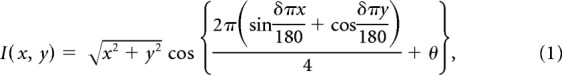where I is the intensity of a pixel with coordinates x and y relative to the center of the screen, and the other parameters, θ and δ, configure the phase and spatial frequency of the pattern. The θ parameter varied across time from 0 to 4π in 72 equal steps of 32 ms duration and thus completed one cycle approximately every 1.15 s. The final parameter, δ, was a function of θ:

Pixel intensities, I, were then rectified such that all positive values were set to white (1997.5 cd/m²) and all negative and zero values were set to black (1.3 cd/m²) presented against a uniform gray background (547.5 cd/m²).

During the mapping runs, participants fixated centrally while a bar (width: 1.5°) containing the ripple pattern traversed the visual field in 24 discrete steps of 0.75°, one per fMRI image acquired. The bar was oriented either vertically or horizontally, and moved in opposite directions in separate sweeps. Each run contained four sweeps of the bar, one for each direction/orientation, and two blank periods. Each sweep or blank period lasted 61.2 s. The order of orientations was different in the four runs, but the blank periods always occurred after the second and the fourth sweep. The bar (and ripple pattern) only ever covered a circular region with a radius of 9° visual angle around fixation, so that it was bounded by the outer edge of this circle. At the edges of the bar and the bounding circular region, the contrast of the ripple pattern was ramped linearly down to zero over a range of 0.28° (Fig. 1). During the HRF measurement run, we presented the full-scale version of the ripple pattern, i.e., a circular region with a radius of 9° visual angle around fixation. In each trial, the stimulus appeared for 2.55 s followed by a blank period of 28.05 s. There were 10 trials in the run.

Figure 1.

Illustration of the mapping stimulus used. Each panel illustrates one trial (only 3 trials are shown but a run comprised six trials). Within a trial of the pRF mapping runs a bar swept across the visual field (in 24 discrete step of half a bar width) in four cardinal directions. The third and sixth trial in each run always contained a blank period. The order of sweep directions varied between runs. During HRF runs the full-field version of this stimulus is how the stimuli would appear to participants.

The fixation dot in all runs was a blue circle (diameter: 0.23°) surrounded by a gap region with background gray (diameter: 1.17°) placed in the center of the screen. In the outer 0.28° of this gap, the contrast of the stimuli was also ramped down to zero. In addition, to facilitate fixation stability throughout the run a low-contrast “radar screen” pattern covered the entire screen: there were 12 radial lines extending from just outside the fixation dot to a maximum eccentricity of 12° (the horizontal edge of the screen). These “spokes” were equally spaced by 30° of polar angle, thus corresponded to analog clock positions. There were also 11 concentric rings centered on fixation increasing in radius in equal steps of 1.09°. Parts of this pattern therefore extended beyond the vertical edges of the screen.

After every 200 ms, the fixation dot could change color to purple with a probability of 0.05 and then change back to blue after 200 ms. Color changes would never occur in immediate succession. Participants were instructed to press a button on an MRI-compatible response box whenever they noticed a color change. Stimuli were projected on a screen at the back of the scanner bore and participants viewed them via a front-surface mirror mounted over the headcoil. All stimuli were generated in MATLAB R2012a (MathWorks) and displayed using the Psychtoolbox package (3.0.10).

Data acquisition.

We acquired fMRI data in a Siemens 3T TIM-Trio scanner using a 32-channel head coil. Because the top half of the coil restricted the participants' field of view this was removed during the functional scans leaving 20 effective channels. Participants lay supine inside the bore and viewed visual stimuli presented on a screen at the bore via a mirror mounted on top of the head coil.

We acquired functional data using a gradient echo planar imaging sequence (2.3 mm isotropic resolution, 30 transverse slices per volume, acquired in interleaved order and centered on the occipital cortex;, matrix size: 96 × 96, slice acquisition time: 85 ms, TE: 37 ms, TR: 2.55 s). We obtained 148 volumes per mapping run and 124 volumes per HRF run. Further, we used a double-echo FLASH sequence short TE: 10 ms, long TE: 12.46 ms, 3 × 3 × 2 mm, 1 mm gap) to acquire B0 field maps to correct for inhomogeneity in the B0 magnetic field. For an initial coregistration of functional and structural images, we acquired a T1-weighted structural image without the front part of the head coil, using a magnetization-prepared rapid acquisition with gradient echo sequence (1 mm isotropic resolution, 176 sagittal slices, matrix size 256 × 215, TE 2.97 ms, TR 1900 ms). Subsequently, we used the full 32-channel head coil with a 3D modified driven equilibrium Fourier transform sequence (1 mm isotropic resolution, 176 sagittal partitions, matrix size 256 × 240, TE: 2.48 ms, TR: 7.92 ms, TI: 910 ms) for cortical reconstruction.

During scanning we acquired data for eye position and pupil size using an EyeLink 1000 MRI compatible eyetracker (http://www.sr-research.com). For technical reasons, reliable eye tracking data could only be collected for 11 ASDs and 8 control participants.

Data analysis.

The first four images in each scanning run were excluded from all further analyses to allow the signal to reach equilibrium. The remaining functional images were preprocessed using SPM8 (Wellcome Trust Centre for Neuroimaging, University College London), including intensity bias correction, slice time correction, motion correction (by realigning images in a two pass procedure, first to the first image acquired, then to the mean across all images from the first pass), unwarping (using B0 field maps to correct for distortion), and coregistration to the T1-weighted structural scans. We first coregistered the functional data to the T1-weighted structural scans acquired without the front part of the head coil, and subsequently all data were coregistered to the second structural scan acquired with the full head coil.

This second T1 structural scan was also used for segmentation and cortical reconstruction (Dale et al., 1999; Fischl et al., 1999) using Freesurfer (version 5.0.0, http://surfer.nmr.mgh.harvard.edu). This creates two 3D surface meshes of each cortical hemisphere, one for the boundary between gray and white matter, and one for the outer (pial) boundary of the white matter. The cortical surfaces were further inflated, smoothing out the cortical curvature and then inflated further to create a spherical model.

All further analyses were performed using custom software developed in the MATLAB programming environment. Functional data were projected onto the gray/white matter surface. At each vertex, we determined the coordinate halfway between the corresponding vertices on the gray/white matter and the pial surfaces and selected this voxel in functional space. This created a functional time series for each vertex. The time series for each run were then z-score normalized and linear detrending was applied.

To estimate each participant's HRF we averaged the time series during each of the 10 trials in the HRF measurement run. Outliers that were further than ±1.5 SDs from the mean were excluded. We then restricted the analysis to all visually active vertices by selecting only those vertices where the average response during first five volumes of each trial after stimulus offset exceeded +1 SEM. Subsequently, we fitted a two-gamma function to estimate the HRF using a simplex search Nelder–Mead algorithm (Nelder and Mead, 1965; Lagarias et al., 1998) to minimize the residual sum of squares. There were four free parameters, the peak amplitude of the function, the ratio of the amplitudes of the two component functions, as well the latency for the initial response and the undershoot.

For pRF analysis we concatenated all the runs acquired with the bar mapping stimulus. We used a forward modeling approach similar to the one described by Dumoulin and Wandell (Dumoulin and Wandell, 2008; Harvey and Dumoulin, 2011) to estimate the pRF parameters for each vertex. The pRF was modeled as a two-dimensional Gaussian in visual space with four free parameters: x and y describes the pRF center position in Cartesian coordinates relative to fixation, σ denotes the SD of the Gaussian, reflecting the spatial spread of the pRF, and β is the response amplitude. In a further analysis we used a difference-of-Gaussians pRF model (cf. Zuiderbaan et al., 2012 for a similar analysis) that incorporates an excitatory center and a larger, inhibitory surround. Here the pRF was modeled with two separate SDs for the center and surround Gaussians, respectively, and an amplitude ratio for the two Gaussians relative to each other. Thus, this model required fitting six free parameters. We used the linear overlap between the pRF model and a binary mask of the stimulus across time (where each 200 × 200 pixel frame corresponds to the stimulus presented during one fMRI volume) to predict the response of neuronal population at each vertex. This predicted neural response was then further convolved with each participant's specific HRF.

To reduce problems with local minima we first conducted an exhaustive grid search. We applied heavy smoothing (Gaussian kernel with FWHM >8.3 mm) to the functional data overlaid on the spherical surface model. We then calculated the Pearson correlation between the time series from each vertex and a search grid comprising 15 × 15 × 34 combinations of x, y, and σ, and selected the combination of parameters resulting in the maximal correlation. The use of Pearson correlation obviated the need to model the signal amplitude of the response. Subsequently, we used these parameters as seeds for an optimization procedure (simplex search algorithm using the Nelder–Mead algorithm) to fit the pRF parameters to the unsmoothed time series for each vertex by minimizing the residual sum of squares between the predicted and observed time series. This model fitting stage included the β parameter for the amplitude. In the difference-of-Gaussians pRF model we used the coarse fitting parameters from the standard Gaussian pRF model to seed the optimization procedure, which then fitted the six parameters of the difference-of-Gaussians model.

Finally, we applied another smoothing step along the spherical surface (Gaussian kernel with FWHM of 5 mm) to the parameter maps. This was to ensure a smooth gradient of the maps based on the assumption that retinotopic organization is macroscopically smooth. This is particularly important for the calculation of cortical surface area and the area subtended by each face in the surface mesh in visual space, and for making inferences of eccentricity-dependent effects. Generally, it is a way to deal with gaps within a map comprising vertices of poor model fits. We calculated a local cortical magnification factor (CMF; Harvey and Dumoulin, 2011) by dividing the square root of visual area (as determined by distances of each pRF to the pRF positions of its cortical neighbors) by the corresponding square root of the cortical surface area calculated in the same way.

Visual regions were delineated manually in Freesurfer by displaying pseudo-color coded maps of polar angle and eccentricity maps calculated from the pRF locations. We delineated V1–V3 according to standard criteria using the reversals in the polar angle map (DeYoe et al., 1994; Sereno et al., 1995; Engel et al., 1997). We further delineated V4 and V3A as full hemifield representations adjacent to the ventral and dorsal portions, respectively, of V3 (Wandell et al., 2007). Finally, we also delineated a region corresponding to MT+ by selecting a region centered on a representation of the upper vertical meridian and extending in an anterior and posterior direction to include two lower vertical meridians (Amano et al., 2009). The anterior portion could only be identified in the subset of participants. These regions likely correspond to areas TO1 and TO2. Both previous literature (Amano et al., 2009) and further experiments of our own (data not shown) showed that this region also corresponded to a cluster of vertices showing a significantly stronger response to moving than static dot stimuli.

We then extracted the vertices labeled in each region (separately for each hemisphere). To measure the macroscopic surface area of a region we summed the area estimates of all vertices whose pRF locations fell between 2° and 7° eccentricity. We further subdivided the vertex data into 1° wide eccentricity bands within a range of 1° and 8° eccentricity. Only vertices with a goodness of fit, R² > 0.1 were included in any further analyses. To make inferences about pRF model parameters, we calculated the mean of each parameter estimate for each bin, averaged these bins across participants in each group, and plotted this group averages against eccentricity. Statistical inferences of differences between the groups were conducted in two ways. First, we simply compared parameters in each bin at the second (group) level using independent sample t tests. Because pRF parameters can show substantial interindividual variability in the normal population (Harvey and Dumoulin, 2011), we confirmed the results of these bin-wise comparisons also using more robust, nonparametric resampling methods. In one instance of these tests, we resampled participants 1000 times (with and without replacement) from the combined sample into two groups of the same size (n = 14 and 12 for ASDs and controls, respectively) and then recalculated the t tests for each bin on each iteration. We estimated statistical significance as the proportion of iterations in which the absolute effect size was larger than the observed one. In another resampling analysis, we instead resampled two groups exclusively from the control group. Resampling in this analysis was always done with replacement. This analysis tested the assumption that a random selection of normal participants could have resulted in the observed differences.

Second, we fitted a cumulative Gaussian curve to the group averages for pRF size σ as a function of eccentricity ρ:

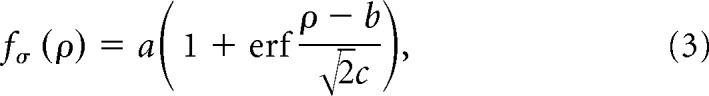where a determines the amplitude of the curve, b its horizontal shift, and c its slope. Similarly, we fitted an exponential decay function to the CMF group averages as a function of eccentricity ρ:

where m determines the amplitude of the curve, k the decay factor, and l the level at which the curve asymptotes. For the amplitude ratios of the difference-of-Gaussians model, we used a simple linear function with a slope and an intercept. We then calculated the difference in these parameters between the two groups and further bootstrapped these fits by resampling each group 1000 times with replacement, refitting the curves, and recalculating the differences between parameters for each iteration. Subsequently, we calculated the proportion of bootstrapped differences in parameters that were opposite to the observed difference. The same procedure was also applied to the squared area under the fitted curves to estimate differences in the overall magnitude of the curves.

For visualization purposes only, we spatially normalized the pRF parameter maps for each participant by resampling them to the template brain “fsaverage” provided within the Freesurfer package. This allowed us to display average retinotopic maps (polar angle, eccentricity, pRF size, goodness-of-fit) on a template brain.

Behavioral experiments.

After completing the MRI scan session, all participants were further tested in a darkened room on short psychophysical experiments. The aim of these experiments was to quickly assess some measures of visual function. Therefore, they were not extensive psychophysical experiments and we neither strongly controlled viewing distance (∼57 cm) nor were participants instructed to maintain fixation. The experiments were performed in a darkened room. As during scanning stimuli were displayed by a desktop computer on an LCD display (Samsung SM2233RZ; refresh rate, 60 Hz) using MATLAB and Psychtoolbox. The luminance range of the display was not linearized.

We used a simple two-down, one-up staircase procedure to test thresholds for discriminating the orientation of a small Gabor patch and the direction of motion of a field of dots. In addition, we used two interleaved one-down, one-up staircases to measure the strength of the Ebbinghaus illusion. In all staircases, we subsequently determined the threshold performance by removing the signal of all reversals outside ±2 median absolute deviations from the median across reversals. Pilot experiments and visual inspection of the data confirmed that this was a robust and precise approach to determine and less susceptible to short-term fluctuation than simply calculating the mean across a final set of reversals. There were 100 trials in each staircase.

In the orientation discrimination experiment we used the method of constant stimuli. After a 100 ms blank period, in each trial a Gabor patch (SD, 1.38°; carrier wavelength, 0.28°) appeared on a gray background (luminance, 76 cd/m²) for 300 ms followed by another blank interval (500 ms) after which a test Gabor appeared (300 ms). The first Gabor was always oriented at 45°, whereas the second could be rotated either clockwise or anticlockwise (counterbalanced, pseudorandomized order). The amount of rotation was controlled by the staircase and the participants were instructed to respond (either by pressing a key on a keyboard or by vocalizing to the experimenter) which way the second Gabor was rotated relative to the first. The angle of rotation always started at 15° and became progressively smaller. It was fixed to be a maximal 30° and minimally 0.5°. Up to the fifth reversal of the staircase, the angle changed by 1°; after that, the angle changed by 0.5°.

In the direction discrimination experiment we used the method of single stimuli and instructed participants to respond whether on average the field of dots was moving to the left or the right. There were 800 dots on a black background (0.6 cd/m²). The average direction of motion was always either left or right (counterbalanced, pseudorandomized order) but random noise drawn from a Gaussian distribution was added to the direction of each dot. The staircase procedure controlled the SD of this noise distribution. It started at zero and progressively increased if participants responded correctly up to a maximal 90°. Up to the fifth reversal, the noise changed by 5°; after that, it changed by 2.5°. This gives a measure of the threshold level of directional uncertainty in the stimulus that a participant can tolerate. We chose this measure because it might be a better estimate of global motion sensitivity than measuring motion coherence because a coherence task could simply be solved by a local strategy, for example counting the number of signal dots. However, in prior pilot experiments we found a close correlation between thresholds for motion coherence and on this directional uncertainty measure. The dots had a diameter of 0.33° and moved with a speed of 8.3°/s. They remained on screen for 300 ms with unlimited lifetime. In the center of the screen there was also a white fixation dot (diameter, 0.16°), although we did not instruct participants to fixate.

For testing the Ebbinghaus illusion, we used a classical illusion stimulus comprising one target disc on a black background (0.6 cd/m²) surrounded by an annulus of 16 smaller discs (disc diameter, 0.4°; distance of disc centers from target center, 1.6°), and one target disc surrounded by an annulus of 6 larger discs (diameter, 3.5°; distance, 3.7°). These two components of the illusion stimulus were presented in left and right halves of the screen on the horizontal meridian centered at an eccentricity of 4.97°. The side on which each component appeared was counterbalanced and pseudorandomized across trials. The target surrounded by small discs was the test stimulus that varied in size, whereas the other target always remained fixed as the reference (diameter, 1.77°). There were two randomly interleaved staircases, one that started with the test being larger (diameter, 2.64°) than the reference, and the other started with the test being smaller (diameter, 1.19°). Participants were instructed to respond which of the targets was larger. Each time they responded correctly/incorrectly, the size ratio of test and reference would decrease/increase (by 0.04 in natural logarithmic units up to the fifth reversal and by 0.02 units afterward). The estimates of illusion strength for the two independent staircases were very reliable (ASD: r = 0.94, p < 10⁻⁵; controls: r = 0.98, p < 10⁻⁷; pooled: r = 0.96, p < 10⁻¹⁴).

Results

We acquired retinotopic mapping data using fMRI on a group of participants with ASDs and matched, neurotypical controls. Figure 2 shows maps for polar angle, eccentricity, and pRF size averaged within each group. Maps in each participant were spatially aligned to a spherical template of the cortical surface. Only the left hemisphere is shown here but very similar maps were seen in the right hemisphere. Reliable retinotopic organization was evident in both groups of participants, with no clear qualitative differences in terms of the macroscopic architecture of the visual regions between groups (Fig. 2A,B). However, pRF sizes in extrastriate regions were qualitatively larger in the ASD group than in controls (Fig. 2C).

Figure 2.

Maps for polar angle (A), eccentricity (B), and pRF size (C) on a spherical model of an anatomical template left cortical surface (see Materials and Methods). Maps from individual participants were spatially normalized by registering their cortical surfaces to the template. Data were then averaged within each group. Left, ASDs. Right, Neurotypical controls. The boundaries of visual regions included in the analysis are indicated on each map. These are based on the group polar map (A) and only for illustration. For analysis, the regions were delineated in native space separately for each participant. Only regions that could be identified in every participant are shown here. The length of the boundaries indicates the extent of an area.

Next, we quantified these parameters by calculating them at a single-participant level (in native space). There were no differences between groups in the macroscopic surface area of any region (independent samples t tests, all p > 0.15), including V1. Neither were there any differences when the surface area of each region was normalized by expressing it as a percentage of overall cortical area (p > 0.0648). Even though ASDs have been linked with anomalies in overall brain size (Courchesne, 2004; Courchesne et al., 2007), we also confirmed that there was no significant difference in the overall cortical surface area between the groups (t₍₂₄₎ = 1.46, p = 0.157).

Focusing on the fine-grained functional architecture, however, revealed considerable differences between groups in extrastriate cortex, in particular at perifoveal eccentricities. Generally, pRF sizes increased as expected with eccentricity and across the visual processing hierarchy (Fig. 3A,C). However, pRF sizes in ASDs were significantly larger than those in controls as evidenced by significantly greater area under the cumulative Gaussian curves fitted to the relationship between pRF size and eccentricity in V2 (bootstrap test: p = 0.001), V3 (p = 0.002), V4 (p = 0.001), and MT+ (p = 0.009) although the latter did not survive Bonferroni correction for multiple comparisons (α = 0.0083). There were no significant differences in V1 (p = 0.207) or V3A (p = 0.376), and there were no differences in terms of any single coefficient of the curves (all p > 0.025) except for the amplitude (p = 0.008) in V4. These findings were further supported by significant binwise differences in the same regions from ∼3–4° eccentricity using both parametric t tests and more robust, nonparametric resampling approaches (see Materials and Methods). These results suggest that autism may be associated with a coarser representation of the perifoveal visual field in extrastriate areas.

Figure 3.

pRF size (A, C) and cortical magnification factors (B, D) averaged across each group and plotted against eccentricity for early (A, B) and higher visual areas (C, D). pRF became larger with greater eccentricity, whereas cortical magnification decreased. However, in V2 and V3 there were also differences between groups in both measures. PRF sizes were also larger in V4 and MT+. Symbols denote the mean in each eccentricity band, solid lines are curves fitted to these data. Error bars denote ±1SEM (errors were typically smaller than the symbol size). Warm colors, ASD group; cold colors, controls. A, B, Circles, V1; diamonds, V2; squares, V3. C, D, Circles, V3A; diamonds, V4; squares, MT+.

We further compared the CMF at each eccentricity between groups (Fig. 3B,D). As expected, CMF decayed exponentially with increasing eccentricity. In V2 and V3, there was a significant difference between groups in both the amplitude (V2, p = 0.001; V3, p < 0.001) and decay factor (V2, p = 0.002; V3, p = 0.003) of the exponential fit. This was likely driven entirely by more centrally biased magnification factors in ASDs at 1°, the most central eccentricity band tested although these differences did not survive correction for multiple comparisons (V2: t₍₂₂₎ = 2.39, p = 0.026; V3: t₍₂₄₎ = 2.82, p = 0.009). There were no differences in the level where the function asymptotes in any area and there were no other differences in any other region.

We also observed subtly greater responses to the mapping stimuli (β parameter in pRF model) in ASDs compared with controls for at least half of eccentricities tested (t tests for each eccentricity band, uncorrected statistical threshold) in V2 (≥5.5° eccentricity, all p < 0.042) and V3 (≥4.5° eccentricity, all p < 0.03). This pattern of results relatively closely followed the pRF size differences (Fig. 4A,C). To ensure that our finding of larger pRFs in autism was not trivially explained by the reliability of model fits, we assessed the goodness of fit, quantified by the coefficient of determination, R², for each region (Fig. 4B,D). In V2 model fits were significantly better in the ASD group than in controls beyond an eccentricity of 6° (all p < 0.011). In V3 there was only a significant difference at 6.5° eccentricity (p = 0.019). We did however not find the same in any other regions (all other p > 0.053). Poor model fits are typically associated with larger pRF sizes, making it unlikely that greater pRFs in ASDs were artifactual (and note that most of these differences would not survive correction for multiple comparisons).

Figure 4.

Beta estimates (A, C) and goodness-of-fit for the pRF model (B, D) averaged across each group and plotted against eccentricity for early (A, B) and higher visual areas (C, D). Beta estimates were slightly larger in the ASD group in many of the same regions as the pRF differences we observed. Symbols denote the mean in each eccentricity band. Error bars denote ±1 SEM. Warm colors, ASD group; cold colors, controls. A, B, Circles, V1; diamonds, V2; squares, V3. C, D, Circles, V3A; diamonds, V4; squares, MT+.

Enlarged pRF sizes could reflect larger neuronal receptive fields and/or increased positional scatter of neuronal receptive fields within a voxel. However, an alternative explanation for larger pRFs in the Gaussian model could be that contextual interactions, in particular surround suppression, are abnormal in ASDs, which would be consistent with reports of an atypical excitatory/inhibitory balance in autism (Foss-Feig et al., 2013; Robertson et al., 2013b). To test for this we conducted an additional analysis. We refitted the data using a center-surround pRF model, based on a difference-of-Gaussians profile comprising a small excitatory center and a larger inhibitory surround (cf. Zuiderbaan et al., 2012 for a similar analysis). This largely confirmed our main findings from the standard two-dimensional Gaussian pRF model (Fig. 5). The size of the central part of the pRF (Fig. 5A) was significantly enlarged in ASDs in V2 (bootstrap test, p = 0.002) and V3 (p < 0.0001). In V4 and MT+ the same trend was observed although these differences were not significant (V4, p = 0.106; MT+, p = 0.044). Critically, the sizes of the inhibitory surrounds (Fig. 5B) were not significantly different in any region (all p > 0.104) and neither were the amplitude ratios (Fig. 5C) of the two component Gaussians (all p > 0.088). Finally, the β parameters for this pRF model (Fig. 5D) confirmed the subtly larger signal strength in ASDs we observed using the standard pRF model. Betas were significantly greater in ASDs in V2 and V3 from 6° eccentricity (largest p = 0.0051).

Figure 5.

Results from difference-of-Gaussians pRF model. Only results from V1–V3 are shown but the pattern is comparable in higher regions. pRF center size (A), surround size (B), surround/center amplitude ratio (C), and β parameters (D) are plotted against eccentricity. All other conventions are the same as in Figures 3 and 4.

We also tested whether our spherical smoothing algorithm distorted the results. The inflation of the folded cortical surface to a sphere may have resulted in different warping factors in the two groups, leading in turn to effective smoothing kernels of different sizes. Such a possibility would be consistent with previous reports of structural differences in occipital cortex between ASDs and neurotypical individuals (Ecker et al., 2010). However, this is unlikely to have affected our results, due to the absence of any macroscopic differences in cortical surface area between groups in the present study. We nonetheless repeated our pRF analysis using unsmoothed data. This essentially corroborated the main results except that the difference in pRF sizes in V3 was now no longer significant after multiple comparison correction (p = 0.047). The other regions, however, showed the same pattern as the main analysis with significant differences in most extrastriate areas (V2, p = 0.001; V4, p < 0.0001; MT+, p = 0.001) but no differences in V1 (p = 0.01) or V3A (p = 0.04). Small differences for unsmoothed data are to be expected because parameter estimates are necessarily more variable in such an analysis.

We further investigated whether differences in the shape or amplitude of the hemodynamic response could have affected our results. There were no significant differences in the average response at each volume in the HRF measurement (Fig. 6A) even at a relaxed uncorrected statistical threshold (t test at each volume, all p > 0.051). Similarly, there were no differences in the fitted parameters of the HRF model (all p > 0.061), except for the overall amplitude being significantly greater in ASDs (t₍₂₄₎ = 2.2, p = 0.037) although this difference did not survive correction for multiple comparisons. The HRF had been quantified using all visual responsive voxels in the functional volume. However, the pattern of results was virtually the same when restricting the HRF comparison separately to each region of interest (Fig. 6B,C). Qualitatively similar results were seen for earlier and higher visual regions, although the relatively small number of voxels in higher regions resulted in relatively large variability there.

Figure 6.

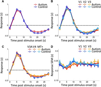
A–C, Hemodynamic response functions for all visually responsive voxels (A) and separately for each of the early visual areas, V1–V3, (B) and V3A-MT+ (C). The response to a 2.55 s visual stimulus is plotted against time. D, SEM of the response in each participant at each time point, averaged across participants in each group, plotted against time. Error bars denote ±1 SEM across participants. Warm colors, ASD group; cold colors, controls. B, Circles, V1; diamonds, V2; squares, V3. C, Circles, V3A; diamonds, V4; squares, MT+.

Eye tracking during the mapping experiment confirmed that there were no significant differences in the variability of eye fixation positions between groups (horizontal position: t₍₁₇₎ = 0.36, p = 0.721; vertical position: t₍₁₇₎ = 0.49, p = 0.631) or in terms of pupil dilation (t₍₁₇₎ = −1.36, p = 0.191). Similarly, we quantified the amount of head motion by extracting the motion parameters from realignment. There were also no significant differences in the mean SD in head translation (x-axis: t₍₂₄₎ = 1.75, p = 0.093; y-axis: t₍₂₄₎ = 0.56, p = 0.578; z-axis: t₍₂₄₎ < 0.01, p = 0.997) or rotation (pitch: t₍₂₄₎ = 0.88, p = 0.388; roll: t₍₂₄₎ = 1.69, p = 0.104 yaw: t₍₂₄₎ = 1.7, p = 0.101) between groups. Finally, analysis of the behavioral performance in the central fixation task revealed no significant differences (hit rate: t₍₂₁₎ = −1.02, p = 0.32; false alarm rate: t₍₂₁₎ = 0.9, p = 0.378). Performance was close to ceiling levels for most participants with high mean hit rates (ASD, 0.85; controls, 0.89) and very low false alarm rates (ASD, 0.002; controls, 0.001).

Previous research reported increased variability in cortical responses to sensory stimulation in ASD participants (Dinstein et al., 2012). We tested whether this could also be observed in our participants. For this analysis, we concentrated on the HRF measurement run because this sparse event-related design is more amenable for this purpose than the more complex pRF mapping design. We found no significant group differences in the SEM in response amplitudes across trials (Fig. 6D), averaged across participants, at any time point (t tests for each volume, all p > 0.111).

We also conducted an exploratory analysis to test whether individual differences in pRF size could be predicted by the severity of autistic symptoms. In V3, the region with the largest differences in pRF size between groups, we found that the average pRF size across the mapped eccentricity range correlated significantly with the AQ of participants [ASD: r = 0.563, p = 0.036 uncorrected, bootstrapped 95% confidence interval (−0.09, 0.95); controls: r = 0.585, p = 0.046 uncorrected (0.38, 0.92)].

Because Pearson correlation can be highly susceptible to the effects of influential bivariate outliers, we further compared the 95% confidence intervals estimated through bootstrapping with the nominal confidence interval expected for these correlations and sample sizes under parametric test assumptions. This revealed considerable deviations suggesting that outliers may have influenced these results. We therefore applied a robust test of association that uses Spearman's ρ after removing outliers based on the bootstrapped Mahalanobis distance (Shepherd's π test; Schwarzkopf et al., 2012). This not only confirmed the relationship between pRF size and AQ but suggested that outliers may have masked its strength (π = 0.8, p < 0.0001 Bonferroni corrected by number of areas and groups). A similar positive correlation was seen in all other tests but none of these were statistically significant, which may be unsurprising due to the small sample sizes. Scatter plots illustrating these correlations are shown in Figure 7.

Figure 7.

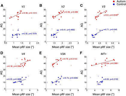
Individual AQ scores plotted against pRF size averaged across each region of interest for V1 (A), V2 (B), V3 (C), V4 (D), V3A (E), and MT+ (F). Statistics in each panel show the strength of robust correlation between variables for each group. Each circle denotes results from one participant; open circles denote outliers rejected by the robust correlation test. Red, ASD group; blue, neurotypical controls. The solid lines indicate the best fitting linear model to the data.

Finally, we also collected behavioral data outside the scanner to test three visual perceptual functions that have been suggested to be atypical in ASDs: discrimination thresholds for global motion direction (Fig. 8A) and orientation (Fig. 8B), and the magnitude of the Ebbinghaus illusion (Fig. 8C). Because such thresholds are frequently not normally distributed, we used nonparametric statistics to compare the median measures for each test (Mann–Whitney U test). We found no significant group differences in orientation thresholds or Ebbinghaus illusion magnitude (orientation, p = 0.939; Ebbinghaus, p = 0.849); however, the discrimination thresholds for global motion direction were significantly worse (p = 0.012) in ASDs compared with controls replicating earlier reports (Spencer et al., 2000; Robertson et al., 2012). This difference was robust to the exclusion of a likely outlier with very poor direction discrimination (p = 0.019). None of the behavioral measures predicted the variability in pRF size in any region (all p > 0.098).

Figure 8.

Behavioral perceptual measures. Threshold uncertainty (SD) in global direction discrimination (A), threshold angle in orientation discrimination (B), and the magnitude (point of subjective equality) of the Ebbinghaus illusion (C) for both groups. Large circles and solid line, median; small circles, individual participants. A, One outlier with a direction uncertainty threshold <60° was excluded from ASD group. C, One ASD participant could not perform the Ebbinghaus task.

Discussion

Consistent with previous research (Hadjikhani et al., 2004), our experiments revealed no differences in macroscopic retinotopic organization in autism spectrum disorders compared with neurotypical controls. However, pRF sizes in extrastriate cortex were significantly enlarged in autism. Interestingly, pRF sizes, at least in V3, also predicted individual differences in autistic traits quantified by the AQ.

To test whether abnormal surround suppression could explain these results, we also fitted a pRF model that explicitly characterized surround suppression. We observed no differences between groups in the width or the strength of surround suppression. However, although pRFs estimated with fMRI show good correspondence with measures based on electrophysiology (Winawer et al., 2011), the relationship between single neuron response properties and pRF parameters measured with fMRI remains unresolved. At the level of fMRI signals, our data indicate that surround suppression does not confound our findings; however, it remains possible that surround suppression at the single neuron level differs between groups.

Visual cortex in ASDs may also be hyper-responsive (Samson et al., 2012). Greater fMRI responses to visual stimulation outside the pRF center would be reflected in larger pRF size estimates. Consistent with this, we observed subtly greater mapping signals (β estimates) throughout extrastriate cortex. We also observed a similar difference in HRF amplitudes. Hyper-responsiveness accords with reports of a reduced ability to filter out task-irrelevant distractors and reduced perceptual load effects on visual processing (Remington et al., 2012) and fMRI responses (Ohta et al., 2012). Unlike previous reports (Dinstein et al., 2012), in our data the variability of fMRI responses to stimulation was not greater in ASDs than in controls: pRF model fits were better in autism compared with controls suggesting a greater signal-to-noise ratio. Hyper-responsive cortical functioning could result from an atypical balance between excitatory and inhibitory processing in primary sensory circuits (Foss-Feig et al., 2013; Robertson et al., 2013b), although others have failed to find such an imbalance in autism (Said et al., 2013). It could also result from abnormal regulatory functions, e.g., reduced adaptation or homeostatic effects.

Alternatively, autism may be associated with a cognitive style where individuals deploy more spatially focused attention to visual stimuli. Enhanced attentional focus on the center of gaze and withdrawal of resources from the surrounding visual field (where the mapping stimuli were located) may result precisely in the blurring of the functional representation of the unattended space and enhanced cortical magnification of the (attended) central visual field. During pRF mapping, participants performed a very simple task at fixation. Behavioral performance was unsurprisingly at ceiling levels for both groups. Nevertheless, it is possible that individuals with autism may engage a more focused attentional “spotlight.” The attentional gradient induced in a cuing paradigm is sharper in autism than in neurotypical controls (Robertson et al., 2013a). Naturally, our task differs from these behavioral experiments, as any attentional resources should be deployed voluntarily in our design.

Although our results cannot conclusively adjudicate between attentional factors or hyper-responsive cortex underlying atypical visual processing in ASDs, our results speak clearly against sharper spatial selectivity of the visual cortex in autism. We observed differences throughout most of extrastriate regions, but no effect in V1. Attentional effects are frequently stronger in higher regions than earlier visual cortex (Maunsell and Cook, 2002). However, if our results reflect differences in responsiveness, this could suggest that higher-level visual functions, such as grouping and object recognition, may be atypical in ASDs, Whichever of these two factors underlies our findings, the correlation between pRF size effects and AQ, an index of the severity of behavioral autistic traits that includes questions on aspects, such as one's attention to detail or the ability to switch the attentional focus, further support the interpretation that our neuroimaging findings are linked to differences in behavior.

Our findings thus provide evidence that spatial selectivity in autism is not generally sharper, ruling out that explanation for atypical perceptual processing reported in individuals with ASDs (Happé, 1996; Rinehart et al., 2000; Spencer et al., 2000; Dakin and Frith, 2005; Simmons et al., 2009; Robertson et al., 2012). Instead, they may point toward potential differences in either the response properties in visual cortex and/or a different cognitive style. Testing a subset of perceptual functions implicated to be abnormal in ASDs, we however found no differences in basic orientation discrimination ability or in the strength of the Ebbinghaus illusion, where the context in which an object appears alters the perception of its size. We did confirm a well replicated finding of decreased ability to discriminate global motion signals (Spencer et al., 2000; Robertson et al., 2012). Yet none of these perceptual functions showed any significant relationship with pRF size differences.

The absence of psychophysical differences could stem from the fact that ASDs comprise a highly heterogeneous group of symptoms. Our experiments were limited to individuals with high-functioning autism and Asperger's syndrome. This reduces the prevalence of comorbid conditions and substantially increases the compliance of participants with experimental procedures. Effects of head or eye motion during the MRI scans can greatly confound neuroimaging results, especially important in-group comparisons. Our inclusion criteria minimized such effects (and our analysis suggests these factors did not confound the results); however, it also opens the possibility that this reduces genuine differences compared with if we had included a broader range of the autism spectrum. Our high-functioning sample may also explain differences to previous studies on ASDs.

A sharpened attentional gradient could in fact explain the lack of differences in orientation thresholds and Ebbinghaus illusion magnitude. Our experiments used fast thresholding procedures with the (perhaps naive) aim to collect perceptual measures in a special population without extensive psychophysical testing. We did not measure eye movements or require participants maintain fixation during these tests. It is feasible that attentional engagement on these local targets permitted all participants to perform at similar levels. Moreover, the forced choice procedure we used to measure illusion strength is not entirely robust against cognitive biases in response criterion (Morgan et al., 2012). We cannot rule out that ASD participants may have responded in a way that mimics the normal illusion. Improved techniques for measuring subjective perception that are impervious to response bias may help address this question in future work.

In our data, the most robust test comparing local and global visual processing was probably the measurement of global motion discrimination. The threshold estimated in these experiments was an objective measure of perceptual sensitivity and it taps into the process of global perception by requiring the observer to average (Robertson et al., 2012) the motion signals over a large region of visual space. Similar findings have been reported previously (Spencer et al., 2000) and at least for global motion discrimination the critical factor may be stimulus duration (Robertson et al., 2012).

Ultimately, further research will be needed to conclusively determine whether attentional deployment rather than general sensory responsiveness are atypical in autism. Our design did not seek to manipulate attention specifically but we simply used a paradigm that moderately engages participants' attentional resources and helps them maintain stable eye fixation. Future mapping studies must seek to compare the effects of directly manipulating spatial attention in autism and controls. However, our findings clearly demonstrate that autism is not characterized by generally finer spatial tuning that could explain enhanced local perceptual processing.

Notes

Supplemental material for this article is available at http://www.fil.ion.ucl.ac.uk/∼sschwarz/Ripples.gif. Animated full-field version illustrating the “ripple” stimulus. This was how the stimulus would appear during HRF measurement runs (presentation duration 2.55 s). During pRF mapping runs the stimulus would be viewed through bar apertures as seen in Figure 1. (Note that the speed of the movie may not be accurate in this illustration). This material has not been peer reviewed.

References

- Amano K, Wandell BA, Dumoulin SO. Visual field maps, population receptive field sizes, and visual field coverage in the human MT+ complex. J Neurophysiol. 2009;102:2704–2718. doi: 10.1152/jn.00102.2009. [DOI] [PMC free article] [PubMed] [Google Scholar]
- Baron-Cohen S, Wheelwright S, Skinner R, Martin J, Clubley E. The autism-spectrum quotient (AQ): evidence from Asperger syndrome/high-functioning autism, males and females, scientists and mathematicians. J Autism Dev Disord. 2001;31:5–17. doi: 10.1023/A:1005653411471. [DOI] [PubMed] [Google Scholar]
- Cherkassky VL, Kana RK, Keller TA, Just MA. Functional connectivity in a baseline resting-state network in autism. Neuroreport. 2006;17:1687–1690. doi: 10.1097/01.wnr.0000239956.45448.4c. [DOI] [PubMed] [Google Scholar]
- Chouinard PA, Noulty WA, Sperandio I, Landry O. Global processing during the Müller-Lyer illusion is distinctively affected by the degree of autistic traits in the typical population. Exp Brain Res. 2013;230:219–231. doi: 10.1007/s00221-013-3646-6. [DOI] [PubMed] [Google Scholar]
- Courchesne E. Brain development in autism: early overgrowth followed by premature arrest of growth. Ment Retard Dev Disabil Res Rev. 2004;10:106–111. doi: 10.1002/mrdd.20020. [DOI] [PubMed] [Google Scholar]
- Courchesne E, Pierce K, Schumann CM, Redcay E, Buckwalter JA, Kennedy DP, Morgan J. Mapping early brain development in autism. Neuron. 2007;56:399–413. doi: 10.1016/j.neuron.2007.10.016. [DOI] [PubMed] [Google Scholar]
- Dakin S, Frith U. Vagaries of visual perception in autism. Neuron. 2005;48:497–507. doi: 10.1016/j.neuron.2005.10.018. [DOI] [PubMed] [Google Scholar]
- Dale AM, Fischl B, Sereno MI. Cortical surface-based analysis: I. Segmentation and surface reconstruction. Neuroimage. 1999;9:179–194. doi: 10.1006/nimg.1998.0395. [DOI] [PubMed] [Google Scholar]
- DeYoe EA, Bandettini P, Neitz J, Miller D, Winans P. Functional magnetic resonance imaging (FMRI) of the human brain. J Neurosci Methods. 1994;54:171–187. doi: 10.1016/0165-0270(94)90191-0. [DOI] [PubMed] [Google Scholar]
- Dinstein I, Heeger DJ, Lorenzi L, Minshew NJ, Malach R, Behrmann M. Unreliable evoked responses in autism. Neuron. 2012;75:981–991. doi: 10.1016/j.neuron.2012.07.026. [DOI] [PMC free article] [PubMed] [Google Scholar]
- Dumoulin SO, Wandell BA. Population receptive field estimates in human visual cortex. Neuroimage. 2008;39:647–660. doi: 10.1016/j.neuroimage.2007.09.034. [DOI] [PMC free article] [PubMed] [Google Scholar]
- Duncan RO, Boynton GM. Cortical magnification within human primary visual cortex correlates with acuity thresholds. Neuron. 2003;38:659–671. doi: 10.1016/S0896-6273(03)00265-4. [DOI] [PubMed] [Google Scholar]
- Duncan RO, Boynton GM. Tactile hyperacuity thresholds correlate with finger maps in primary somatosensory cortex (S1) Cereb Cortex. 2007;17:2878–2891. doi: 10.1093/cercor/bhm015. [DOI] [PubMed] [Google Scholar]
- Ecker C, Marquand A, Mourão-Miranda J, Johnston P, Daly EM, Brammer MJ, Maltezos S, Murphy CM, Robertson D, Williams SC, Murphy DG. Describing the brain in autism in five dimensions: magnetic resonance imaging-assisted diagnosis of autism spectrum disorder using a multiparameter classification approach. J Neurosci. 2010;30:10612–10623. doi: 10.1523/JNEUROSCI.5413-09.2010. [DOI] [PMC free article] [PubMed] [Google Scholar]
- Engel SA, Glover GH, Wandell BA. Retinotopic organization in human visual cortex and the spatial precision of functional MRI. Cereb Cortex. 1997;7:181–192. doi: 10.1093/cercor/7.2.181. [DOI] [PubMed] [Google Scholar]
- Fischl B, Sereno MI, Dale AM. Cortical surface-based analysis: II. Inflation, flattening, and a surface-based coordinate system. Neuroimage. 1999;9:195–207. doi: 10.1006/nimg.1998.0396. [DOI] [PubMed] [Google Scholar]
- Foss-Feig JH, Tadin D, Schauder KB, Cascio CJ. A substantial and unexpected enhancement of motion perception in autism. J Neurosci. 2013;33:8243–8249. doi: 10.1523/JNEUROSCI.1608-12.2013. [DOI] [PMC free article] [PubMed] [Google Scholar]
- Hadjikhani N, Chabris CF, Joseph RM, Clark J, McGrath L, Aharon I, Feczko E, Tager-Flusberg H, Harris GJ. Early visual cortex organization in autism: an fMRI study. Neuroreport. 2004;15:267–270. doi: 10.1097/00001756-200402090-00011. [DOI] [PubMed] [Google Scholar]
- Happé FG. Studying weak central coherence at low levels: children with autism do not succumb to visual illusions: a research note. J Child Psychol Psychiatry. 1996;37:873–877. doi: 10.1111/j.1469-7610.1996.tb01483.x. [DOI] [PubMed] [Google Scholar]
- Harvey BM, Dumoulin SO. The relationship between cortical magnification factor and population receptive field size in human visual cortex: constancies in cortical architecture. J Neurosci. 2011;31:13604–13612. doi: 10.1523/JNEUROSCI.2572-11.2011. [DOI] [PMC free article] [PubMed] [Google Scholar]
- Lagarias J, Reeds J, Wright M, Wright P. Convergence properties of the Nelder–Mead simplex method in low dimensions. SIAM J Optim. 1998;9:112–147. doi: 10.1137/S1052623496303470. [DOI] [Google Scholar]
- Lord C, Risi S, Lambrecht L, Cook EH, Jr, Leventhal BL, DiLavore PC, Pickles A, Rutter M. The autism diagnostic observation schedule-generic: a standard measure of social and communication deficits associated with the spectrum of autism. J Autism Dev Disord. 2000;30:205–223. doi: 10.1023/A:1005592401947. [DOI] [PubMed] [Google Scholar]
- Maunsell JH, Cook EP. The role of attention in visual processing. Philos Trans R Soc Lond B Biol Sci. 2002;357:1063–1072. doi: 10.1098/rstb.2002.1107. [DOI] [PMC free article] [PubMed] [Google Scholar]
- Morgan M, Dillenburger B, Raphael S, Solomon JA. Observers can voluntarily shift their psychometric functions without losing sensitivity. Atten Percept Psychophys. 2012;74:185–193. doi: 10.3758/s13414-011-0222-7. [DOI] [PMC free article] [PubMed] [Google Scholar]
- Nelder JA, Mead R. A simplex method for function minimization. Comput J. 1965;7:308–313. doi: 10.1093/comjnl/7.4.308. [DOI] [Google Scholar]
- Ohta H, Yamada T, Watanabe H, Kanai C, Tanaka E, Ohno T, Takayama Y, Iwanami A, Kato N, Hashimoto RI. An fMRI study of reduced perceptual load-dependent modulation of task-irrelevant activity in adults with autism spectrum conditions. Neuroimage. 2012;61:1176–1187. doi: 10.1016/j.neuroimage.2012.03.042. [DOI] [PubMed] [Google Scholar]
- Rajimehr R, Tootell RB. Does retinotopy influence cortical folding in primate visual cortex? J Neurosci. 2009;29:11149–11152. doi: 10.1523/JNEUROSCI.1835-09.2009. [DOI] [PMC free article] [PubMed] [Google Scholar]
- Remington AM, Swettenham JG, Lavie N. Lightening the load: perceptual load impairs visual detection in typical adults but not in autism. J Abnorm Psychol. 2012;121:544–551. doi: 10.1037/a0027670. [DOI] [PMC free article] [PubMed] [Google Scholar]
- Rinehart NJ, Bradshaw JL, Moss SA, Brereton AV, Tonge BJ. Atypical interference of local detail on global processing in high-functioning autism and Asperger's disorder. J Child Psychol Psychiatry. 2000;41:769–778. doi: 10.1111/1469-7610.00664. [DOI] [PubMed] [Google Scholar]
- Robertson CE, Martin A, Baker CI, Baron-Cohen S. Atypical integration of motion signals in autism spectrum conditions. PloS One. 2012;7:e48173. doi: 10.1371/journal.pone.0048173. [DOI] [PMC free article] [PubMed] [Google Scholar]
- Robertson CE, Kravitz DJ, Freyberg J, Baron-Cohen S, Baker CI. Tunnel vision: sharper gradient of spatial attention in autism. J Neurosci. 2013a;33:6776–6781. doi: 10.1523/JNEUROSCI.5120-12.2013. [DOI] [PMC free article] [PubMed] [Google Scholar]
- Robertson CE, Kravitz DJ, Freyberg J, Baron-Cohen S, Baker CI. Slower rate of binocular rivalry in autism. J Neurosci. 2013b;33:16983–16991. doi: 10.1523/JNEUROSCI.0448-13.2013. [DOI] [PMC free article] [PubMed] [Google Scholar]
- Said CP, Egan RD, Minshew NJ, Behrmann M, Heeger DJ. Normal binocular rivalry in autism: implications for the excitation/inhibition imbalance hypothesis. Vision Res. 2013;77:59–66. doi: 10.1016/j.visres.2012.11.002. [DOI] [PMC free article] [PubMed] [Google Scholar]
- Samson F, Mottron L, Soulières I, Zeffiro TA. Enhanced visual functioning in autism: an ALE meta-analysis. Hum Brain Mapp. 2012;33:1553–1581. doi: 10.1002/hbm.21307. [DOI] [PMC free article] [PubMed] [Google Scholar]
- Schwarzkopf DS, Rees G. Subjective size perception depends on central visual cortical magnification in human v1. PloS One. 2013;8:e60550. doi: 10.1371/journal.pone.0060550. [DOI] [PMC free article] [PubMed] [Google Scholar]
- Schwarzkopf DS, Song C, Rees G. The surface area of human V1 predicts the subjective experience of object size. Nat Neurosci. 2011;14:28–30. doi: 10.1038/nn.2706. [DOI] [PMC free article] [PubMed] [Google Scholar]
- Schwarzkopf DS, De Haas B, Rees G. Better ways to improve standards in brain-behavior correlation analysis. Front Hum Neurosci. 2012;6:200. doi: 10.3389/fnhum.2012.00200. [DOI] [PMC free article] [PubMed] [Google Scholar]
- Sereno MI, Dale AM, Reppas JB, Kwong KK, Belliveau JW, Brady TJ, Rosen BR, Tootell RB. Borders of multiple visual areas in humans revealed by functional magnetic resonance imaging. Science. 1995;268:889–893. doi: 10.1126/science.7754376. [DOI] [PubMed] [Google Scholar]
- Simmons DR, Robertson AE, McKay LS, Toal E, McAleer P, Pollick FE. Vision in autism spectrum disorders. Vision Res. 2009;49:2705–2739. doi: 10.1016/j.visres.2009.08.005. [DOI] [PubMed] [Google Scholar]
- Song C, Schwarzkopf DS, Rees G. Variability in visual cortex size reflects tradeoff between local orientation sensitivity and global orientation modulation. Nat Commun. 2013;4:2201. doi: 10.1038/ncomms3201. [DOI] [PMC free article] [PubMed] [Google Scholar]
- Soulières I, Dawson M, Samson F, Barbeau EB, Sahyoun CP, Strangman GE, Zeffiro TA, Mottron L. Enhanced visual processing contributes to matrix reasoning in autism. Hum Brain Mapp. 2009;30:4082–4107. doi: 10.1002/hbm.20831. [DOI] [PMC free article] [PubMed] [Google Scholar]
- Spencer J, O'Brien J, Riggs K, Braddick O, Atkinson J, Wattam-Bell J. Motion processing in autism: evidence for a dorsal stream deficiency. Neuroreport. 2000;11:2765–2767. doi: 10.1097/00001756-200008210-00031. [DOI] [PubMed] [Google Scholar]
- Van Essen DC. A tension-based theory of morphogenesis and compact wiring in the central nervous system. Nature. 1997;385:313–318. doi: 10.1038/385313a0. [DOI] [PubMed] [Google Scholar]
- Wandell BA, Dumoulin SO, Brewer AA. Visual field maps in human cortex. Neuron. 2007;56:366–383. doi: 10.1016/j.neuron.2007.10.012. [DOI] [PubMed] [Google Scholar]
- Wechsler D. Wechsler adult intelligence scale (WAIS) Ed 3. London: Psychological; 1999a. [Google Scholar]
- Wechsler D. Wechsler abbreviated scale of intelligence (WASI) San Antonio, TX: Harcourt Assessment; 1999b. [Google Scholar]
- Winawer J, Rauschecker AM, Parvizi J, Wandell BA. Population receptive fields in human visual cortex measured with subdural electrodes. J Vis. 2011;11(11):1196. doi: 10.1167/11.11.1196. [DOI] [Google Scholar]
- Zuiderbaan W, Harvey BM, Dumoulin SO. Modeling center-surround configurations in population receptive fields using fMRI. J Vis. 2012;12(3):10. doi: 10.1167/12.3.10. [DOI] [PubMed] [Google Scholar]