Coupled dimensionality reduction and classification for supervised and semi-supervised multilabel learning

Abstract

Coupled training of dimensionality reduction and classification is proposed previously to improve the prediction performance for single-label problems. Following this line of research, in this paper, we first introduce a novel Bayesian method that combines linear dimensionality reduction with linear binary classification for supervised multilabel learning and present a deterministic variational approximation algorithm to learn the proposed probabilistic model. We then extend the proposed method to find intrinsic dimensionality of the projected subspace using automatic relevance determination and to handle semi-supervised learning using a low-density assumption. We perform supervised learning experiments on four benchmark multilabel learning data sets by comparing our method with baseline linear dimensionality reduction algorithms. These experiments show that the proposed approach achieves good performance values in terms of hamming loss, average AUC, macro F₁, and micro F₁ on held-out test data. The low-dimensional embeddings obtained by our method are also very useful for exploratory data analysis. We also show the effectiveness of our approach in finding intrinsic subspace dimensionality and semi-supervised learning tasks.

1. Introduction

Multilabel learning considers classification problems where each data point is associated with a set of labels simultaneously instead of just a single label (Tsoumakas et al., 2009). This setup can be handled by training distinct classifiers for each label separately (i.e., assuming no correlation between the labels). However, exploiting the correlation information between the labels may improve the overall prediction performance. There are two common approaches for exploiting this information: (i) joint learning of the model parameters of distinct classifiers trained for each label (Boutell et al., 2004; Zhang and Zhou, 2007; Sun et al., 2008; Petterson and Caetano, 2010; Guo and Gu, 2011; Zhang, 2011; Zhang et al., 2011) and (ii) learning a shared subspace and doing classification in this subspace (Yu et al., 2005; Park and Lee, 2008; Ji and Ye, 2009; Rai and Daumé III, 2009; Ji et al., 2010; Wang et al., 2010; Zhang and Zhou, 2010). In this paper, we are focusing on the second approach.

Dimensionality reduction algorithms try to achieve two main goals: (i) removing the inherent noise to improve the prediction performance and (ii) obtaining low-dimensional visualizations for exploratory data analysis. Principal component analysis (PCA) (Pearson, 1901) and linear discriminant analysis (LDA) (Fisher, 1936) are two well-known algorithms for unsupervised and supervised dimensionality reduction, respectively.

We can use any unsupervised dimensionality reduction algorithm for multilabel learning. However, the key idea in multilabel learning is to use the correlation information between the labels and we only consider supervised dimensionality reduction algorithms. As an early attempt, Yu et al. (2005) propose a supervised latent semantic indexing variant that makes use of multiple labels. Park and Lee (2008) and Wang et al. (2010) modify LDA algorithm for multilabel learning. Rai and Daumé III (2009) propose a probabilistic canonical correlation analysis method that can also be applied in semi-supervised settings. Ji et al. (2010) and Zhang and Zhou (2010) formulate multilabel dimensionality reduction as an eigenvalue problem that uses input features and class labels together.

For supervised learning problems, dimensionality reduction and prediction steps are generally performed separately with two different target functions, leading to low prediction performance. Hence, coupled training of these two steps may improve the overall system performance. Biem et al. (1997) propose a multilayer perceptron variant that performs coupled feature extraction and classification. Coupled training of the projection matrix and the classifier is also studied in the framework of support vector machines by introducing the projection matrix into the optimization problem solved (Chapelle et al., 2002; Pereira and Gordon, 2006). Gönen and Alpaydm (2010) introduce the same idea to a localized multiple kernel learning framework to capture multiple modalities that may exist in the data. There are also metric learning methods that try to transfer the neighborhood in the input space to the projected subspace in nearest neighbor settings (Goldberger et al., 2005; Globerson and Roweis, 2006; Weinberger and Saul, 2009). Sajama and Orlitsky (2005) use mixture models for each class to obtain better projections, whereas Mao et al. (2010) use them on both input and output data. The resulting projections found by these approaches are not linear and they can be regarded as manifold learning methods. Yu et al. (2006) propose a supervised probabilistic PCA and an efficient solution method, but the algorithm is developed only for real outputs. Rish et al. (2008) formulate a supervised dimensionality reduction algorithm coupled with generalized linear models for binary classification and regression, and maximize a target function composed of input and output likelihood terms using an iterative algorithm.

In this paper, we propose novel supervised and semi-supervised multilabel learning methods where the linear projection matrix and the binary classification parameters are learned together to maximize the prediction performance in the projected subspace. We make the following contributions: In Section 2, we give the graphical model of our approach for supervised multilabel learning called Bayesian supervised multilabel learning (BSML) and introduce a deterministic variational approximation for inference. Section 3 formulates our two variants: (i) BSML with automatic relevance determination (BSML+ARD) to find intrinsic dimensionality of the projected subspace and (ii) Bayesian semi-supervised multilabel learning (BSSML) to make use of unlabeled data. In Section 4, we discuss the key properties of our algorithms. Section 5 tests our algorithms on four benchmark multilabel data sets in different settings.

2. Coupled dimensionality reduction and classification for supervised multilabel learning

Performing dimensionality reduction and classification successively (with two different objective functions) may not result in a predictive subspace and may have low generalization performance. In order to find a better subspace, coupling dimensionality reduction and single-output supervised learning is previously proposed (Biem et al., 1997; Chapelle et al., 2002; Goldberger et al., 2005; Sajama and Orlitsky, 2005; Globerson and Roweis, 2006; Pereira and Gordon, 2006; Yu et al., 2006; Rish et al., 2008; Weinberger and Saul, 2009; Gönen and Alpaydm, 2010; Mao et al., 2010). We should consider the predictive performance of the target subspace while learning the projection matrix. In order to benefit from the correlation between the class labels in a multilabel learning scenario, we assume a common subspace and perform classification for all labels in that subspace using different classifiers for each label separately. The predictive quality of the subspace now depends on the prediction performances for multiple labels instead of a single one.

Figure 1 illustrates the probabilistic model for multilabel binary classification with a graphical model and its distributional assumptions. The data matrix X is used to project data points into a low-dimensional space using the projection matrix Q. The low-dimensional representations of data points Z and the classification parameters {b, W} are used to calculate the classification scores. Finally, the given class labels Y are generated from the auxiliary matrix T, which is introduced to make the inference procedures efficient (Albert and Chib, 1993). We formulate a variational approximation procedure for inference in order to have a computationally efficient algorithm.

Figure 1.

Coupled dimensionality reduction and classification for supervised multilabel learning.

The notation we use throughout the manuscript is given in Table 1. The superscripts index the rows of matrices, whereas the subscripts index the columns of matrices and the entries of vectors. As short-hand notations, all priors in the model are denoted by Ξ = {λ, Φ, Ψ}, where the remaining variables by Θ = {b, Q, T, W, Z} and the hyper-parameters by ζ = {α_λ, β_λ, α_ϕ, β_ϕ, α_ψ, β_ψ}. Dependence on ζ is omitted for clarity throughout the manuscript. N(·; μ, Σ) denotes the normal distribution with the mean vector μ and the covariance matrix Σ. G(·; α, β) denotes the gamma distribution with the shape parameter α and the scale parameter β. δ(·) denotes the Kronecker delta function that returns 1 if its argument is true and 0 otherwise.

Table 1.

List of notation.

D	Input space dimensionality
N	Number of training instances
R	Projected subspace dimensionality
L	Number of output labels
X ∈ ℝD×N	Data matrix (i.e., collection of training instances)
Q ∈ ℝD×R	Projection matrix (i.e., dimensionality reduction parameters)
Φ ∈ ℝD×R	Priors for projection matrix (i.e., precision priors)
Z ∈ ℝR×N	Projected data matrix (i.e., low-dimensional representation of instances)
W ∈ ℝL×R	Weight matrix (i.e., classification parameters for labels)
Ψ ∈ ℝL×R	Priors for weight matrix (i.e., precision priors)
b ∈ ℝL	Bias vector (i.e., bias parameters for labels)
λ ∈ ℝL	Priors for bias vector (i.e., precision priors)
T ∈ ℝL×N	Auxiliary matrix (i.e., discriminant outputs)
Y ∈ {±1}L×N	Label matrix (i.e., true labels of training instances)

2.1. Inference using variational approximation

The variational methods use a lower bound on the marginal likelihood using an ensemble of factored posteriors to find the joint parameter distribution (Beal, 2003). Assuming independence between the approximate posteriors in the factorable ensemble can be justified because there is not a strong coupling between our model parameters. We can write the factorable ensemble approximation of the required posterior as

$$p(\mathbf{\Theta },\mathbf{\Xi }\mid \mathbf{X},\mathbf{Y})\approx q(\mathbf{\Theta },\mathbf{\Xi })=q(\mathbf{\Phi })q(\mathbf{Q})q(\mathbf{Z})q(\mathit{\lambda })q(\mathbf{\Psi })q(\mathit{b},\mathbf{W})q(\mathbf{T})$$

and define each factor in the ensemble just like its full conditional distribution:

$$\begin{array}{lll}q(\mathbf{\Phi })& =& \prod _{f=1}^D\prod _{s=1}^{R}G({\varphi }_s^f;\alpha ({\varphi }_s^f),\beta ({\varphi }_s^f))\\ q(\mathbf{Q})& =& \prod _{s=1}^{R}N({\mathit{q}}_s;\mu ({\mathit{q}}_s),\mathrm{\sum }({\mathit{q}}_s))\\ q(\mathbf{Z})& =& \prod _{i=1}^{N}N({\mathit{z}}_i;\mu ({\mathit{z}}_i),\mathrm{\sum }({\mathit{z}}_i))\\ q(\mathit{\lambda })& =& \prod _{o=1}^{L}G({\lambda }_o;\alpha ({\lambda }_o),\beta ({\lambda }_o))\\ q(\mathbf{\Psi })& =& \prod _{o=1}^L\prod _{s=1}^{R}G({\psi }_o^s;\alpha ({\psi }_o^s),\beta ({\psi }_o^s))\\ q(\mathit{b},\mathbf{W})& =& \prod _{o=1}^{L}N\left(\left[\begin{array}{c}{b}_o\\ {\mathit{w}}_o\end{array}\right];\mu (b_o,{\mathit{w}}_o),\mathrm{\sum }(b_o,{\mathit{w}}_o)\right)\\ q(\mathbf{T})& =& \prod _{o=1}^L\prod _{i=1}^{N}TN(t_i^o;\mu (t_i^o),\mathrm{\sum }(t_i^o),\rho (t_i^o))\end{array}$$

where α(·), β(·), μ(·), and Σ(·) denote the shape parameter, the scale parameter, the mean vector, and the covariance matrix for their arguments, respectively. TN(·; μ, Σ, ρ(·)) denotes the truncated normal distribution with the mean vector μ, the covariance matrix Σ, and the truncation rule ρ(·) such that TN(·; μ, Σ, ρ(·)) ∝ N(·; μ, Σ) if ρ(·) is true and TN(·; μ, Σ, ρ(·)) = 0 otherwise.

We choose to model projected data instances explicitly (i.e., not marginalizing out them) and independently (i.e., assuming a distribution independent of other variables) in the factorable ensemble approximation in order to decouple the dimensionality reduction and classification parts. By doing this, we achieve to obtain update equations for Q and {b, W} independent of each other.

We can bound the marginal likelihood using Jensen’s inequality:

$$\log p(\mathbf{Y}\mid \mathbf{X})\ge {\mathrm{E}}_{q(\mathbf{\Theta },\mathbf{\Xi })}[\log p(\mathbf{Y},\mathbf{\Theta },\mathbf{\Xi }\mid \mathbf{X})]-{\mathrm{E}}_{q(\mathbf{\Theta },\mathbf{\Xi })}[\log q(\mathbf{\Theta },\mathbf{\Xi })]$$ (1)

and optimize this bound by optimizing with respect to each factor separately until convergence. The approximate posterior distribution of a specific factor τ can be found as

$$q(\mathit{\tau })\propto \exp ({\mathrm{E}}_{q(\{\mathbf{\Theta },\mathbf{\Xi }\}\backslash \mathit{\tau })}[\log p(\mathbf{Y},\mathbf{\Theta },\mathbf{\Xi }\mid \mathbf{X})]).$$

For our model, thanks to the conjugacy, the resulting approximate posterior distribution of each factor follows the same distribution as the corresponding factor.

2.2. Inference details

The approximate posterior distribution of the priors of the precisions for the projection matrix can be found as a product of gamma distributions:

$$q(\mathbf{\Phi })=\prod _{f=1}^D\prod _{s=1}^{R}G({\varphi }_s^f;{\alpha }_{\varphi }+1/2,{(1/{\beta }_{\varphi }+\langle {(q_s^f)}^2\rangle /2)}^{-1})$$ (2)

where the tilde notation denotes the posterior expectations as usual, i.e., 〈f(τ)〉 = E_q(τ)[f (τ)]. The approximate posterior distribution of the projection matrix is a product of multivariate normal distributions:

$$q(\mathbf{Q})=\prod _{s=1}^{R}N\left({\mathit{q}}_s;\mathrm{\sum }({\mathit{q}}_s)\mathbf{X}\langle {\mathit{z}}^s\rangle ,{(\mathrm{diag}(\langle {\varphi }_{\mathit{s}}\rangle )+{\mathbf{XX}}^{\top })}^{-1}\right).$$ (3)

The approximate posterior distribution of the projected instances can also be formulated as a product of multivariate normal distributions:

$$q(\mathbf{Z})=\prod _{i=1}^{N}N\left({\mathit{z}}_i;\mathrm{\sum }({\mathit{z}}_i)\left(\langle {\mathbf{Q}}^{\top }\rangle {\mathit{x}}_i+\sum _{o=1}^L(\langle {\mathit{w}}_o\rangle \langle t_i^o\rangle -\langle {\mathit{w}}_o{b}_o\rangle )\right),{\left(\mathbf{I}+\sum _{o=1}^L\langle {\mathit{w}}_o{\mathit{w}}_o^{\top }\rangle \right)}^{-1}\right)$$ (4)

where the classification parameters and the auxiliary variables defined for each label are used together.

The approximate posterior distributions of the priors on the biases and the weight vectors can be found as products of gamma distributions:

$$q(\mathit{\lambda })=\prod _{o=1}^{L}G({\lambda }_o;{\alpha }_{\lambda }+1/2,{(1/{\beta }_{\lambda }+\langle b_o^2\rangle /2)}^{-1})$$ (5)

$$q(\mathbf{\Psi })=\prod _{o=1}^L\prod _{s=1}^{R}G({\psi }_o^s;{\alpha }_{\psi }+1/2,{(1/{\beta }_{\psi }+\langle {(w_o^s)}^2\rangle /2)}^{-1}).$$ (6)

The approximate posterior distribution of the classification parameters is a product of multivariate normal distributions:

$$q(\mathit{b},\mathbf{W})=\prod _{o=1}^{L}N\left(\left[\begin{array}{c}{b}_o\\ {\mathit{w}}_o\end{array}\right];\mathrm{\sum }(b_o,{\mathit{w}}_o)\left[\begin{array}{c}{\mathbf{1}}^{\top }\langle {\mathit{t}}_o\rangle \\ \langle \mathbf{Z}\rangle \langle {\mathit{t}}_o\rangle \end{array}\right],{\left[\begin{array}{cc}\langle {\lambda }_o\rangle +N& {\mathbf{1}}^{\top }\langle {\mathbf{Z}}^{\top }\rangle \\ \langle \mathbf{Z}\rangle \mathbf{1}& \mathrm{diag}(\langle {\mathit{\psi }}_o\rangle )+\langle {\mathbf{ZZ}}^{\top }\rangle \end{array}\right]}^{-1}\right).$$ (7)

The approximate posterior distribution of the auxiliary variables is a product of truncated normal distributions:

$$q(\mathbf{T})=\prod _{o=1}^L\prod _{i=1}^N\mathit{TN}(t_i^o;\langle {\mathit{w}}_o^{\top }\rangle \langle {\mathit{z}}_i\rangle +\langle b_o\rangle ,1,t_i^o{y}_i^o>0)$$ (8)

where we need to find the posterior expectations in order to update the approximate posterior distributions of the projected instances and the classification parameters. Fortunately, the truncated normal distribution has a closed-form formula for its expectation.

2.3. Complete algorithm

The complete inference algorithm is listed in Algorithm 1. The inference mechanism sequentially updates the approximate posterior distributions of the model parameters and the latent variables until convergence, which can be checked by monitoring the lower bound in (1). Exact form of the variational lower bound can be found in Appendix Appendix A. The first term of the lower bound corresponds to the sum of exponential forms of the distributions in the joint likelihood. The second term is the sum of negative entropies of the approximate posteriors in the ensemble. The only nonstandard distribution in the second term is the truncated normal distributions of the auxiliary variables; nevertheless, the truncated normal distribution has a closed-form formula also for its entropy. The posterior expectations needed for the algorithm can be found in Appendix Appendix B.

Algorithm 1 Bayesian Supervised Multilabel Learning

Require: X, Y, R, αλ, βλ, αϕ, βϕ, αψ, and βψ Initialize q(Q), q(Z), q(b, W), and q(T) randomly repeat  Update q(Φ) and q(Q) using (2) and (3)  Update q(Z) using (4)  Update q(λ), q(Ψ), and q(b, W) using (5), (6), and (7)  Update q(T) using (8) until convergence q(Q) and q(b, W)

2.4. Prediction

In the prediction step, we can replace p(Q∣X, Y) with its approximate posterior distribution q(Q) and obtain the predictive distribution of the projected instance z_* for a new data point x_* as

$$p({\mathit{z}}_{\ast }\mid {\mathit{x}}_{\ast },\mathbf{X},\mathbf{Y})=\prod _{s=1}^{R}N(z_{\ast }^s;\mu {({\mathit{q}}_s)}^{\top }{\mathit{x}}_{\ast },1+x_{\ast }^{\top }\mathrm{\sum }({\mathit{q}}_s){\mathit{x}}_{\ast }).$$

The predictive distribution of the auxiliary variable $t_{\ast }^o$ can also be found by replacing p(b, W∣X, Y) with its approximate posterior distribution q(b, W):

$$p(t_{\ast }^o\mid \mathbf{X},\mathbf{Y},{\mathit{z}}_{\ast })=N\left(t_{\ast }^o;\mu {(b_o,{\mathit{w}}_o)}^{\top }\left[\begin{array}{c}1\\ {\mathit{z}}_{\ast }\end{array}\right],[1{\mathit{z}}_{\ast }]\mathrm{\sum }(b_o,{\mathit{w}}_o)\left[\begin{array}{c}1\\ {\mathit{z}}_{\ast }\end{array}\right]+1\right)\forall o$$

and the predictive distribution of the class label $y_{\ast }^o$ can be formulated using the auxiliary variable distribution:

$$p(y_{\ast }^o=+1\mid {\mathit{x}}_{\ast },\mathbf{X},\mathbf{Y})=\mathbf{\Phi }(\mu (t_{\ast }^o)/\mathrm{\sum }(t_{\ast }^o))\forall o$$

where Φ(·) is the standardized normal cumulative distribution function.

3. Extensions

This section introduces two variants derived from the base model we describe above.

3.1. Finding intrinsic subspace dimensionality using automatic relevance determination

The dimensionality of the projected subspace is generally selected using a cross-validation strategy or is fixed before learning. Instead of these two naive approaches, the intrinsic subspace dimensionality of the data can be identified while learning the model parameters. The typical choice is to use ARD (Neal, 1996) that defines independent multivariate Gaussian priors on the columns of the projection matrix.

The distributional assumptions for the column-wise prior case can be given as

$$\begin{array}{cc}{\varphi }_s~G({\varphi }_s;{\alpha }_{\varphi },{\beta }_{\varphi })& \forall s\hfill \\ q_s^f\mid {\varphi }_s~N(q_s^f;0,{\varphi }_s^{-1})& \forall (f,s)\hfill \end{array}$$

and the approximate posterior distributions of the priors and the projection matrix become

$$\begin{array}{lll}q(\varphi )& =& \prod _{s=1}^{R}G\left({\varphi }_s;{\alpha }_{\varphi }+D/2,{(1/{\beta }_{\varphi }+\langle {\mathit{q}}_s^{\top }{\mathit{q}}_s\rangle /2)}^{-1}\right)\\ q(\mathbf{Q})& =& \prod _{s=1}^{R}N({\mathit{q}}_s;\mathrm{\sum }({\mathit{q}}_s)\mathbf{X}\langle {\mathit{z}}^s\rangle ,{(\langle {\varphi }_s\rangle \mathbf{I}+{\mathbf{XX}}^{\top })}^{-1}).\end{array}$$

3.2. Coupled dimensionality reduction and classification for semi-supervised multilabel learning

Labeling large data collections may not be possible due to extensive labour required. In such cases, we should efficiently use a large number of unlabeled data points in addition to a few labeled data points (i.e., semi-supervised learning). Semi-supervised learning is not well-studied in the context of multilabel learning. There are a few attempts that formulate the problem as a matrix factorization problem (Liu et al., 2006; Chen et al., 2008). To our knowledge, Rai and Daumé III (2009), Qian and Davidson (2010), and Guo and Schuurmans (2012) are the only studies that consider dimensionality reduction and classification together for multilabel learning in a semi-supervised setup.

We modify our probabilistic model described above for semi-supervised learning assuming a low-density region between the classes (Lawrence and Jordan, 2005). We basically need to make the class labels partially observed and to introduce a new set of observed auxiliary variables denoted by L. The distributional assumptions for Y and L are defined as follows:

$$\begin{array}{llll}{y}_i^o\mid t_i^o& ~& \{\begin{array}{ll}\delta (y_i^o{t}_i^o>1/2)& y_i^o\in \{\pm 1\}\\ 1-\delta (1/2\ge t_i^o\ge -1/2)& \mathrm{otherwise}\end{array}& \forall (o,i)\\ l_i^o\mid y_i^o& ~& \delta (y_i^o\in \{\pm 1\})& \forall (o,i).\end{array}$$

The first distributional assumption has two main implications: (i) A low-density region is placed between the classes similar to the margin in support vector machines. (ii) Unlabeled data points are forced to be outside of this low-density region.

The approximate posterior distribution of the auxiliary variables can again be formulated as a product of truncated normal distributions:

$$\begin{array}{lll}q(\mathbf{T})& =& \prod _{o=1}^L\prod _{i\in L_o}\mathit{TN}(t_i^o;\langle {\mathit{w}}_o^{\top }\rangle \langle {\mathit{z}}_i\rangle +\langle b_o\rangle ,1,t_i^o{y}_i^o>1/2)\\ & & \prod _{o=1}^L\prod _{i\in u_o}({\gamma }_o^{-}\mathrm{\Phi }(-1/2-\langle {\mathit{w}}_o^{\top }\rangle \langle {\mathit{z}}_i\rangle -\langle b_o\rangle )\mathit{TN}(t_i^o;\langle {\mathit{w}}_o^{\top }\rangle \langle {\mathit{z}}_i\rangle +\langle b_o\rangle ,1,t_i^o<-1/2)\\ & & +{\gamma }_o^{+}\mathrm{\Phi }(\langle {\mathit{w}}_o^{\top }\rangle \langle {\mathit{z}}_i\rangle +\langle b_o\rangle -1/2)\mathit{TN}(t_i^o;\langle {\mathit{w}}_o^{\top }\rangle \langle {\mathit{z}}_i\rangle +\langle b_o\rangle ,1,t_i^o>1/2)){({Ƶ}_i^o)}^{-1}\end{array}$$

where $L_o=\{i:y_i^o\in \{\pm 1\}\}$, $u_o=\{i:y_i^o\notin \{\pm 1\}\}$, ${\gamma }_o^{-}$ is the prior probability of the negative class for label o, ${\gamma }_o^{+}$ is the prior probability of the positive class for label o, and ${Ƶ}_i^o$ is the normalization coefficient calculated for the unlabeled data point x_i and label o. The predictive distribution of the class label $y_{\ast }^o$ can be found as

$$p\left(y_{\ast }^o=+1\mid {\mathit{x}}_{\ast },\mathbf{X},\mathbf{Y}\right)={({Ƶ}_{\ast }^o)}^{-1}\mathrm{\Phi }((\mu (t_{\ast }^o)-1/2)/\mathrm{\sum }(t_{\ast }^o))\forall o$$

where ${Ƶ}_{\ast }^o$ is the normalization coefficient calculated for the test data point x_* and label o.

4. Discussion

The most time-consuming updates of our algorithm are the covariance calculations of (3), (4), and (7) whose time complexities can be given as O(RD³), O(R³), and O(LR³), respectively. If the number of output labels is not very large compared to the input space dimensionality, updating the projection matrix Q using (3) is the most time-consuming step, which requires inverting R different D × D matrices for the covariance calculations and dominates the overall running time. When D is very large, the dimensionality of the input space should be reduced using an unsupervised dimensionality reduction method (e.g., PCA) before running the algorithm. Note that having a large number of training instances does not affect the running time heavily due to simple update rules and posterior expectation calculations for the auxiliary matrix T.

The multiplication of the projection matrix Q and the supervised learning parameters W can be interpreted as the model parameters of linear classifiers for the original representation. However, if the number of output labels is larger than the projected subspace dimensionality (i.e., L > R), the parameter matrix QW is guaranteed to be low-rank due to this decomposition leading to a more regularized solution. For multivariate regression estimation, our model can be interpreted as a full Bayesian treatment of reduced-rank regression (Tso, 1981).

We modify the precision priors for the projection matrix to determine the dimensionality of the projected subspace automatically. These priors can also be modified to decide which features should be used by changing entry-wise priors on the projection matrix with row-wise sparse priors. This formulation allows us to perform feature selection and multilabel classification at the same time.

5. Experiments

We use four widely used benchmark data sets, namely, Emotions, Scene, TMC2007, and Yeast, from different domains to compare our algorithms with the baseline algorithms using provided train/test splits. These data sets are publicly available from http://mulan.sourceforge.net/datasets.html and their characteristics can be summarized as:

• Emotions: N_train = 391, N_test = 202, D = 72, and L = 6,

• Scene: N_train = 1211, N_test = 1196, D = 294, and L = 6,

• TMC2007: N_train = 21519, N_test = 7077, D = 500, and L = 22,

• Yeast: N_train = 1500, N_test = 917, D = 103, and L = 14.

Four popular performance measures for multilabel learning, namely, hamming loss, average Area Under the Curve (AUC), macro F₁, and micro F₁ are used to compare the algorithms. Hamming loss is the average classification error over the labels. The smaller the value of hamming loss, the better the performance. Average AUC is the average area under the Receiver Operating Characteristic (ROC) curve over the labels. The larger the value of average AUC, the better the performance. Macro F₁ is the average of F₁ scores over the labels. The larger the value of macro F₁, the better the performance. Micro F₁ calculates the F₁ score over the labels as a whole. The larger the value of micro F₁, the better the performance. We also report training times for all of the algorithms to compare their computational requirements.

5.1. Supervised learning experiments

We test our new algorithm BSML on four different data sets by comparing it with four (one unsupervised and three supervised) baseline dimensionality reduction algorithms, namely, PCA (Pearson, 1901), multilabel dimensionality reduction via dependency maximization (MDDM) (Zhang and Zhou, 2010), multilabel least squares (MLLS) (Ji et al., 2010), and multilabel linear discriminant analysis (MLDA) (Wang et al., 2010). BSML combines dimensionality reduction and binary classification for multilabel learning in a joint framework. In order to have comparable algorithms, we perform binary classification using probit model (PROBIT) on each label separately, after reducing dimensionality using baseline algorithms. The suffix +PROBIT corresponds to learning a binary classifier for each label in the projected subspace using PROBIT. We also report the classification results obtained by training a PROBIT on each label separately without dimensionality reduction to see the baseline performance.

We implement variational approximation methods for both PROBIT and BSML in Matlab, where we take 500 iterations. The default hyper-parameter values for PROBIT and BSML are selected as (α_λ, β_λ, α_ψ, β_ψ) = (1, 1, 1, 1) and (α_λ, β_λ, α_ø, β_ø, α_ψ, β_ψ) = (1, 1, 1, 1, 1, 1), respectively. We implement our own versions for PCA, MDDM, MLLS, and MLDA. We use the provided default parameter values for MDDM, MLLS, and MLDA.

Figure 2 gives the classification results on Emotions data set. We perform experiments with R = 1, 2, …, 6 for all of the methods except MLDA and with R = 1,2, …, 5 for MLDA. Note that the dimensionality of the projected subspace can be at most D for PCA, L − 1 for MLDA, and L for MDDM and MLLS. There is not such a restriction for BSML. We see that BSML clearly outperforms all of the baseline algorithms for all of the dimensions tried in terms of hamming loss and average AUC, and the performance difference is around two per cent when R = 2. BSML results with all of the dimensions tried are better than using the original feature representation without any dimensionality reduction (i.e., PROBIT). However, BSML and MLDA+PROBIT seem comparable in terms of macro F₁ and micro F₁. Both algorithms achieve similar macro F₁ and micro F₁ values as PROBIT using two or more dimensions. When we compare training times, we see that all baseline algorithms are trained in two seconds, whereas PROBIT requires three seconds and BSML takes three to five seconds depending on the subspace dimensionality.

Figure 2.

Comparison of algorithms on Emotions data set.

The classification results on Scene data set are given in Figure 3. We perform experiments with R = 1, 2, …, 6 for all of the methods except MLDA and with R = 1, 2, …, 5 for MLDA. In terms of hamming loss, BSML is better than other dimensionality reduction algorithms with R = 1 and 2. However, MDDM+PROBIT achieves lower hamming loss values after two dimensions. All of the dimensionality reduction algorithms get lower hamming loss and average AUC values than PROBIT after four dimensions. In terms of macro F₁ and micro F₁, BSML is the best algorithm among dimensionality reduction methods up to four dimensions. After four dimensions, MDDM+PROBIT, BSML, MLLS+PROBIT, and MLDA+PROBIT are better than PROBIT in terms of both macro F₁ and micro F₁. All baseline algorithms take less than one minute to train, whereas BSML requires more than one minute only when R = 6.

Figure 3.

Comparison of algorithms on Scene data set.

Figure 4 shows the classification results on TMC2007 data set. We perform experiments with R = 1, 2, …, 22 for all of the methods except MLDA and with R = 1, 2, …, 21 for MLDA. We see that BSML clearly outperforms all of the baseline dimensionality reduction algorithms in terms of hamming loss, average AUC (only when R > 1), macro F₁ (only when R < 13), and micro F₁. However, the performance values are not as good as PROBIT due to the large number of class labels (i.e., L = 22). The performance difference between PROBIT and BSML in terms of hamming loss is around two per cent with only two dimensions. All of the baseline dimensionality reduction algorithms take less than ten minutes to train, whereas PROBIT needs around 25 minutes and BSML requires around one hour when R = 22. This shows that our Bayesian formulation can be scaled up to large data sets with tens of thousands of training instances.

Figure 4.

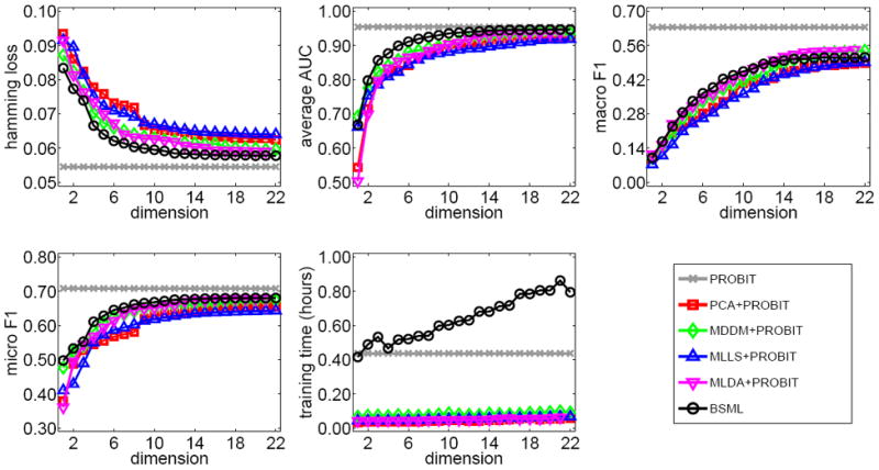
Comparison of algorithms on TMC2007 data set.

The classification results on Yeast data set are shown in Figure 5. We perform experiments with R = 1, 2, …, 14 for all of the methods except MLDA and with R = 1, 2, …, 13 for MLDA. MDDM+PROBIT is the best algorithm in terms of hamming loss for R = 2, whereas BSML is the best one for R = 3 and 4. After four dimensions, there is no clear outperforming algorithm. BSML is the best algorithm in terms of average AUC for R > 2 and it is the only algorithm that obtains consistently better average AUC values than PROBIT. When the projected subspace is two- or three-dimensional, BSML is clearly better than all of the baseline dimensionality reduction algorithms in terms of macro F₁ and micro F₁. We also see that all of the algorithms can be trained under one minute on Yeast data set.

Figure 5.

Comparison of algorithms on Yeast data set.

We use PROBIT to classify projected instances for comparing BSML with baseline dimensionality reduction algorithms in terms of classification performance. This may add some bias to the comparisons because BSML contains PROBIT in its formulation. We also replicate the experiments using k-nearest neighbor as the classification algorithm after dimensionality reduction. The classification performances on the four data sets (not reported here) are very similar to the ones obtained using PROBIT. This shows that the superiority of BSML especially on very low dimensions can not be explained by the use of PROBIT only.

In addition to performing classification, the projected subspace found by BSML can also be used for exploratory data analysis. Figure 6 shows two-dimensional embeddings of training data points and classification boundaries obtained by MLDA and BSML on Emotions data set. The labels of this data set corresponds to different emotions assigned to musical pieces by three experts. We can see that, with two dimensions, BSML achieves to embed data points in a more predictive subspace than MLDA. The correlations between different labels are clearly visible in the embedding obtained, for example, the positive correlation between quiet-still and sad-lonely, and the negative correlation between relaxing-calm and angry-fearful.

Figure 6.

Two-dimensional embeddings obtained by (a) MLDA and (b) BSML on Emotions data set.

5.2. Automatic relevance determination experiments

We perform another set of supervised learning experiments on four benchmark data sets to test whether our method can find the intrinsic subspace dimensionality automatically. We also implement BSML+ARD in Matlab and take 500 iterations for both methods. The default hyper-parameter values for BSML and BSML+ARD are selected as (α_λ, β_λ, α_ϕ, β_ϕ, α_ψ, β_ψ) = (1, 1, 1, 1, 1, 1) and (α_λ, β_λ, α_ϕ, β_ϕ, α_ψ, β_ψ) = (1, 1, 10⁻¹⁰, 10⁺¹⁰, 1, 1), respectively. For each dataset, we set the subspace dimensionality to the number of output labels (i.e., R = L).

The performances of BSML and BSML+ARD on benchmark data sets in terms of hamming loss are as follows:

• Emotions: BSML = 0.2153 and BSML+ARD = 0.2186,

• Scene: BSML = 0.1150 and BSML+ARD = 0.1356,

• TMC2007: BSML = 0.0578 and BSML+ARD = 0.0609,

• Yeast: BSML = 0.2053 and BSML+ARD = 0.2033.

We can see that BSML+ARD achieves comparable hamming loss values with respect to BSML and successfully eliminate some of the dimensions in order to find the intrinsic dimensionality. Two- or three-dimensional subspaces are enough to obtain a good prediction performance on Emotions (uses two dimensions), Scene (uses three dimensions), and Yeast (uses three dimensions) data sets, whereas TMC2007 data set requires eight dimensions.

5.3. Semi-supervised learning experiments

In order to test the performance of BSSML, we perform semi-supervised learning experiments on each data set using the transductive learning setup. We implement BSSML in Matlab and take 500 iterations. The default hyper-parameter values for BSSML are selected as (α_λ, β_λ, α_ϕ, β_ϕ, α_ψ, β_ψ) = (1, 1, 1, 1, 1, 1). We set γ⁻ and γ⁺ to 0.5 not to impose any prior information on the unlabeled data points. We compare our new algorithm BSSML with semi-supervised dimension reduction for multilabel classification (SSDRMC) (Qian and Davidson, 2010). We also implement SSDRMC in Matlab and use the provided default parameter values.

The performances of BSSML and SSDRMC on benchmark data sets in terms of hamming loss are as follows:

• Emotions: SSDRMC = 0.2805 and BSSML = 0.2021,

• Scene: SSDRMC = 0.1345 and BSSML = 0.1164,

• TMC2007: SSDRMC = NA and BSSML = 0.0590,

• Yeast: SSDRMC = 0.2485 and BSSML = 0.2035.

Note that we could not report SSDRMC result on TMC2007 data set due to excessive computational need. We can see that, on Emotions, Scene, and Yeast data sets, BSSML is significantly better than SSDRMC in terms of hamming loss.

6. Conclusions

We present a Bayesian supervised multilabel learning method that couples linear dimensionality reduction and linear binary classification. We then provide detailed derivations for supervised learning using a deterministic variational approximation approach. We also formulate two variants: (i) an automatic relevance determination variant to find intrinsic dimensionality of the projected subspace and (ii) a semi-supervised learning variant with a low-density region between the classes to make use of unlabeled data. Matlab implementations of our algorithms BSML and BSSML are publicly available at http://users.ics.aalto.fi/gonen/bssml/.

Supervised learning experiments on four benchmark multilabel learning data sets show that our model obtains better performance values than baseline linear dimensionality reduction algorithms most of the time. The low-dimensional embeddings obtained by our method can also be used for exploratory data analysis. Automatic relevance determination and semi-supervised learning experiments also show the effectiveness of our formulation in different settings.

The proposed models can be extended in different directions: First, we can use a nonlinear dimensionality reduction step before multilabel classification step using kernels instead of data matrix. Second, we can use a nonlinear classification algorithm such as Gaussian processes instead of probit model in our formulation to increase the prediction performance. Lastly, we can learn a unified subspace for multiple input representations (i.e., multitask learning) by exploiting the correlations between different tasks defined on different input features. This extension also allows us to learn a transfer function between different feature representations (i.e., transfer learning).

• *Introduces a novel Bayesian multilabel learning algorithm
• *Combines dimensionality reduction and classification for (semi-)supervised setup
• *Uses a deterministic variational approximation for efficient inference
• *Achieves good performance values in terms of hamming loss, average AUC, macro F1, and micro F1
• *Obtains very useful low-dimensional embeddings for exploratory data analysis

Appendix A. Variational lower bound

The variational lower bound of our multilabel learning model can be written as

$$L={\mathrm{E}}_{q(\mathbf{\Theta },\mathbf{\Xi })}[\log p(\mathbf{Y},\mathbf{\Theta },\mathbf{\Xi }\mid \mathbf{X})]-{\mathrm{E}}_{q(\mathbf{\Theta },\mathbf{\Xi })}[\log q(\mathbf{\Theta },\mathbf{\Xi })]$$

where the joint likelihood is defined as

$$p(\mathbf{Y},\mathbf{\Theta },\mathbf{\Xi }\mid \mathbf{X})=p(\mathbf{\Phi })p(\mathbf{Q}\mid \mathbf{\Phi })p(\mathbf{Z}\mid \mathbf{Q},\mathbf{X})p(\mathbf{\lambda })p(\mathit{b}\mid \mathbf{\lambda })p(\mathbf{\Psi })p(\mathbf{W}\mid \mathbf{\Psi })p(\mathbf{T}\mid \mathit{b},\mathbf{W},\mathbf{Z})p(\mathbf{Y}\mid \mathbf{T}).$$

Using these definitions, the variational lower bound becomes

$$\begin{array}{lll}L& =& {\mathrm{E}}_{q(\mathbf{\Phi })}[\log p(\mathbf{\Phi })]+{\mathrm{E}}_{q(\mathbf{\Phi })q(\mathbf{Q})}[\log p(\mathbf{Q}\mid \mathbf{\Phi })]+{\mathrm{E}}_{q(\mathbf{Q})q(\mathbf{Z})}[\log p(\mathbf{Z}\mid \mathbf{Q},\mathbf{X})]+{\mathrm{E}}_{q(\mathit{\lambda })}[\log p(\mathit{\lambda })]\\ & & +{\mathrm{E}}_{q(\mathit{\lambda })q(\mathit{b},\mathbf{W})}[\log p(\mathit{b}\mid \mathit{\lambda })]+{\mathrm{E}}_{q(\mathbf{\Psi })}[\log p(\mathbf{\Psi })]+{\mathrm{E}}_{q(\mathbf{\Psi })q(\mathit{b},\mathbf{W})}[\log p(\mathbf{W}\mid \mathbf{\Psi })]\\ & & +{\mathrm{E}}_{q(\mathbf{Z})q(\mathit{b},\mathbf{W})q(\mathbf{T})}[\log p(\mathbf{T}\mid \mathit{b},\mathbf{W},\mathbf{Z})]+{\mathrm{E}}_{q(\mathbf{T})}[\log p(\mathbf{Y}\mid \mathbf{T})]-{\mathrm{E}}_{q(\mathbf{\Phi })}[\log q(\mathbf{\Phi })]-{\mathrm{E}}_{q(\mathbf{Q})}[\log q(\mathbf{Q})]\\ & & -{\mathrm{E}}_{q(\mathbf{Z})}[\log q(\mathbf{Z})]-{\mathrm{E}}_{q(\mathit{\lambda })}[\log q(\mathit{\lambda })]-{\mathrm{E}}_{q(\mathbf{\Psi })}[\log q(\mathbf{\Psi })]-{\mathrm{E}}_{q(\mathit{b},\mathbf{W})}[\log q(\mathit{b},\mathbf{W})]-{\mathrm{E}}_{q(\mathbf{T})}[\log q(\mathbf{T})]\end{array}$$

where the exponential form expectations of the distributions in the joint likelihood can be calculated as

$$\begin{array}{ccc}\hfill {\mathrm{E}}_{q(\mathbf{\Phi })}[\log p(\mathbf{\Phi })]& =& \sum _{f=1}^D\sum _{s=1}^R(({\alpha }_{\varphi }-1)\langle \log {\varphi }_s^f\rangle -\langle {\varphi }_s^f\rangle /{\beta }_{\varphi }-\mathrm{log\; \Gamma }({\alpha }_{\varphi })-{\alpha }_{\varphi }\log {\beta }_{\varphi })\hfill \\ \hfill {\mathrm{E}}_{q(\mathbf{\Phi })q(\mathbf{Q})}[\log p(\mathbf{Q}\mid \mathbf{\Phi })]& =& \sum _{s=1}^R(-\mathrm{tr}(\mathrm{diag}(\langle {\varphi }_s\rangle )\langle {\mathit{q}}_s{\mathit{q}}_s^{\top }\rangle )/2-D\log 2\pi /2+\log |\mathrm{diag}(\langle {\varphi }_s\rangle )|/2)\hfill \\ \hfill {\mathrm{E}}_{q(\mathbf{Q})q(\mathbf{Z})}[\log p(\mathbf{Z}\mid \mathbf{Q},\mathbf{X})]& =& \sum _{i=1}^N(-\langle {\mathit{z}}_i^{\top }{\mathit{z}}_i\rangle /2+\langle {\mathit{z}}_i^{\top }\rangle \langle {\mathbf{Q}}^{\top }\rangle {\mathit{x}}_i-\mathrm{tr}(\langle \mathbf{Q}{\mathbf{Q}}^{\top }\rangle {\mathit{x}}_i{\mathit{x}}_i^{\top })/2-R\log 2\pi /2)\hfill \\ \hfill {\mathrm{E}}_{q(\mathit{\lambda })}[\log p(\mathit{\lambda })]& =& \sum _{o=1}^L(({\alpha }_{\lambda }-1)\langle \log {\lambda }_o\rangle -\langle {\lambda }_o\rangle /{\beta }_{\lambda }-\mathrm{log\; \Gamma }({\alpha }_{\lambda })-{\alpha }_{\lambda }\log {\beta }_{\lambda })\hfill \\ \hfill {\mathrm{E}}_{q(\mathit{\lambda })q(\mathit{b},\mathbf{W})}[\log p(\mathit{b}\mid \mathit{\lambda })]& =& \sum _{o=1}^L(-\langle {\lambda }_o\rangle \langle b_o^2\rangle /2-\log 2\pi /2+\log \langle {\lambda }_o\rangle /2)\hfill \\ \hfill {\mathrm{E}}_{q(\mathbf{\Psi })}[\log p(\mathbf{\Psi })]& =& \sum _{s=1}^R\sum _{o=1}^L(({\alpha }_{\psi }-1)\langle \log {\psi }_o^s\rangle -\langle {\psi }_o^s\rangle /{\beta }_{\psi }-\mathrm{log\; \Gamma }({\alpha }_{\psi })-{\alpha }_{\psi }\log {\beta }_{\psi })\hfill \\ \hfill {\mathrm{E}}_{q(\mathbf{\Psi })q(\mathit{b},\mathbf{W})}[\log p(\mathbf{W}\mid \mathbf{\Psi })]& =& \sum _{o=1}^L(-\mathrm{tr}(\mathrm{diag}(\langle {\psi }_o\rangle )\langle {\mathit{w}}_o{\mathit{w}}_o^{\top }\rangle )/2-R\log 2\pi /2+\log |\mathrm{diag}(\langle {\psi }_o\rangle )|/2)\hfill \\ \hfill {\mathrm{E}}_{q(\mathbf{Z})q(\mathit{b},\mathbf{W})q(\mathbf{T})}[\log p(\mathbf{T}\mid \mathit{b},\mathbf{W},\mathbf{Z})]& =& \sum _{o=1}^L\sum _{i=1}^N(-\langle {(t_i^o)}^2\rangle /2+\langle t_i^o\rangle (\langle {\mathit{w}}_o^{\top }\rangle \langle {\mathit{z}}_i\rangle +\langle b_o\rangle )\hfill \\ & & -(\mathrm{tr}(\langle {\mathit{w}}_o{\mathit{w}}_o^{\top }\rangle \langle {\mathit{z}}_i{\mathit{z}}_i^{\top }\rangle )+2\langle {\mathit{z}}_i^{\top }\rangle \langle {\mathit{w}}_o{b}_o\rangle +\langle b_o^2\rangle )/2-\log 2\pi /2)\hfill \\ \hfill {\mathrm{E}}_{q(\mathbf{T})}[\log p(\mathbf{Y}\mid \mathbf{T})]& =& 0\hfill \end{array}$$

and the negative entropies of the approximate posteriors in the ensemble are given as

$$\begin{array}{ccc}\hfill {\mathrm{E}}_{q(\mathbf{\Phi })}[\log q(\mathbf{\Phi })]& =& \sum _{f=1}^D\sum _{s=1}^R(-\alpha ({\varphi }_s^f)-\log \beta ({\varphi }_s^f)-\mathrm{log\; \Gamma }(\alpha ({\varphi }_s^f))-(1-\alpha ({\varphi }_s^f))\psi (\alpha ({\varphi }_s^f)))\hfill \\ \hfill {\mathrm{E}}_{q(\mathbf{Q})}[\log q(\mathbf{Q})]& =& \sum _{s=1}^R(-D(\log 2\pi +1)/2-\log |\mathrm{\sum }({\mathit{q}}_s)|/2)\hfill \\ \hfill {\mathrm{E}}_{q(\mathbf{Z})}[\log q(\mathbf{Z})]& =& \sum _{i=1}^N(-R(\log 2\pi +1)/2-\log |\mathrm{\sum }({\mathit{z}}_i)|/2)\hfill \\ \hfill {\mathrm{E}}_{q(\mathit{\lambda })}[\log q(\mathit{\lambda })]& =& \sum _{o=1}^L(-\alpha ({\lambda }_o)-\log \beta ({\lambda }_o)-\mathrm{log\; \Gamma }(\alpha ({\lambda }_o))-(1-\alpha ({\lambda }_o))\psi (\alpha ({\lambda }_o)))\hfill \\ \hfill {\mathrm{E}}_{q(\mathbf{\Psi })}[\log q(\mathbf{\Psi })]& =& \sum _{s=1}^R\sum _{o=1}^L(-\alpha ({\psi }_o^s)-\log \beta ({\psi }_o^s)-\mathrm{log\; \Gamma }(\alpha ({\psi }_o^s))-(1-\alpha ({\psi }_o^s))\psi (\alpha ({\psi }_o^s)))\hfill \\ \hfill {\mathrm{E}}_{q(\mathit{b},\mathbf{W})}[\log q(\mathit{b},\mathbf{W})]& =& \sum _{o=1}^L(-(R+1)(\log 2\pi +1)/2-\log |\mathrm{\sum }(b_o,{\mathit{w}}_o)|/2)\hfill \\ \hfill {\mathrm{E}}_{q(\mathbf{T})}[\log q(\mathbf{T})]& =& \sum _{o=1}^L\sum _{i=1}^N(-(\log 2\pi +\mathrm{\sum }(t_i^o))/2-\log {Ƶ}_i^o)\hfill \end{array}$$

where Γ(·) denotes the gamma function and ψ(·) denotes the digamma function.

Appendix B. Posterior expectations

The posterior expectations needed in order to update approximate posterior distributions and to calculate the lower bound can be given as

$$\begin{array}{cccc}\hfill \langle {\varphi }_s^f\rangle & =& \alpha ({\varphi }_s^f)\beta ({\varphi }_s^f)\hfill & \forall (f,s)\hfill \\ \hfill \langle \log {\varphi }_s^f\rangle & =& \psi (\alpha ({\varphi }_s^f))+\log \beta ({\varphi }_s^f)\hfill & \forall (f,s)\hfill \\ \hfill \langle {\varphi }_s\rangle & =& {\left[\alpha ({\varphi }_s^1)\beta ({\varphi }_s^1)\alpha ({\varphi }_s^2)\beta ({\varphi }_s^2)\cdots \alpha ({\varphi }_s^D)\beta ({\varphi }_s^D)\right]}^{\top }\hfill & \forall s\hfill \\ \hfill \langle {(q_s^f)}^2\rangle & =& \mu {(q_s^f)}^2+\mathrm{\sum }(q_s^f)\hfill & \forall (f,s)\hfill \\ \hfill \langle {\mathit{q}}_s\rangle & =& {\left[\mu (q_s^1)\mu (q_s^2)\cdots \mu (q_s^D)\right]}^{\top }\hfill & \forall s\hfill \\ \hfill \langle {\mathit{q}}_s{\mathit{q}}_s^{\top }\rangle & =& \mu ({\mathit{q}}_s)\mu {({\mathit{q}}_s)}^{\top }+\mathrm{\sum }({\mathit{q}}_s)\hfill & \forall s\hfill \\ \hfill \langle \mathbf{Q}\rangle & =& \left[\mu ({\mathit{q}}_1)\mu ({\mathit{q}}_2)\cdots \mu ({\mathit{q}}_R)\right]\hfill & \\ \hfill \langle {\mathbf{QQ}}^{\top }\rangle & =& \sum _{s=1}^R(\mu ({\mathit{q}}_s)\mu {({\mathit{q}}_s)}^{\top }+\mathrm{\sum }({\mathit{q}}_s))\hfill & \\ \hfill \langle {\mathit{z}}^s\rangle & =& \left[\mu (z_1^s)\mu (z_2^s)\cdots \mu (z_N^s)\right]\hfill & \forall s\hfill \\ \hfill \langle {\mathit{z}}_i\rangle & =& {\left[\mu (z_i^1)\mu (z_i^2)\cdots \mu (z_i^R)\right]}^{\top }\hfill & \forall i\hfill \\ \hfill \langle {\mathit{z}}_i^{\top }{\mathit{z}}_i\rangle & =& \sum _{s=1}^R(\mu {(z_i^s)}^2+\mathrm{\sum }(z_i^s))\hfill & \forall i\hfill \\ \hfill \langle {\mathit{z}}_i{\mathit{z}}_i^{\top }\rangle & =& \mu ({\mathit{z}}_i)\mu {({\mathit{z}}_i)}^{\top }+\mathrm{\sum }({\mathit{z}}_i)\hfill & \forall s\hfill \\ \hfill \langle \mathbf{Z}\rangle & =& \left[\mu ({\mathit{z}}_1)\mu ({\mathit{z}}_2)\cdots \mu ({\mathit{z}}_N)\right]\hfill & \\ \hfill \langle {\mathbf{ZZ}}^{\top }\rangle & =& \sum _{i=1}^N(\mu ({\mathit{z}}_i)\mu {({\mathit{z}}_i)}^{\top }+\mathrm{\sum }({\mathit{z}}_i))\hfill & \\ \hfill \langle {\lambda }_o\rangle & =& \alpha ({\lambda }_o)\beta ({\lambda }_o)\hfill & \forall o\hfill \\ \hfill \langle \log {\lambda }_o\rangle & =& \psi (\alpha ({\lambda }_o))+\log \beta ({\lambda }_o)\hfill & \forall o\hfill \\ \hfill \langle {\psi }_o^s\rangle & =& \alpha ({\psi }_o^s)\beta ({\psi }_o^s)\hfill & \forall (s,o)\hfill \\ \hfill \langle \log {\psi }_o^s\rangle & =& \psi (\alpha ({\psi }_o^s))+\log \beta ({\psi }_o^s)\hfill & \forall (s,o)\hfill \\ \hfill \langle {\mathit{\psi }}_o\rangle & =& {\left[\alpha ({\psi }_o^1)\beta ({\psi }_o^1)\alpha ({\psi }_o^2)\beta ({\psi }_o^2)\cdots \alpha ({\psi }_o^R)\beta ({\psi }_o^R)\right]}^{\top }\hfill & \forall o\hfill \\ \hfill \langle b_o\rangle & =& \mu (b_o)\hfill & \forall o\hfill \\ \hfill \langle b_o^2\rangle & =& \mu {(b_o)}^2+\mathrm{\sum }(b_o)\hfill & \forall o\hfill \\ \hfill \langle {(w_o^s)}^2\rangle & =& \mu {(w_o^s)}^2+\mathrm{\sum }(w_o^s)\hfill & \forall (s,o)\hfill \\ \hfill \langle {\mathit{w}}_o\rangle & =& {\left[\mu (w_o^1)\mu (w_o^2)\cdots \mu (w_o^R)\right]}^{\top }\hfill & \forall o\hfill \\ \hfill \langle {\mathit{w}}_o{\mathit{w}}_o^{\top }\rangle & =& \mu ({\mathit{w}}_o)\mu {({\mathit{w}}_o)}^{\top }+\mathrm{\sum }({\mathit{w}}_o)\hfill & \forall o.\hfill \end{array}$$

The only nonstandard distribution we need to operate on is the truncated normal distribution used for the auxiliary variables. From our model definition, the truncation points for each auxiliary variable are defined as

$$(l_i^o,u_i^o)=\{\begin{array}{ll}(-\infty ,0)& \mathrm{if}{y}_i^o=-1\\ (0,+\infty )& \mathrm{otherwise}\end{array}\forall (o,i)$$

where $l_i^o$ and $u_i^o$ denote the lower and upper truncation points, respectively. The normalization coefficient, the expectation, and the variance of the auxiliary variables can be calculated as

$$\begin{array}{cccc}\hfill {Ƶ}_i^o& =& \mathrm{\Phi }({\beta }_i^o)-\mathrm{\Phi }({\alpha }_i^o)\hfill & \forall (o,i)\\ \hfill \langle t_i^o\rangle & =& \langle {\mathit{w}}_o^{\top }\rangle \langle {\mathit{z}}_i\rangle +\langle b_o\rangle +(\varphi ({\alpha }_i^o)-\varphi ({\beta }_i^o))/{Ƶ}_i^o\hfill & \forall (o,i)\\ \hfill \langle {(t_i^o)}^2\rangle -{\left(\langle t_i^o\rangle \right)}^2& =& 1+({\alpha }_i^o\varphi ({\alpha }_i^o)-{\beta }_i^o\varphi ({\beta }_i^o))/{Ƶ}_i^o-{(\varphi ({\alpha }_i^o)-\varphi ({\beta }_i^o))}^2/{({Ƶ}_i^o)}^2\hfill & \forall (o,i)\end{array}$$

where ϕ(·) is the standardized normal probability density function and $\{{\alpha }_i^o,{\beta }_i^o\}$ are defined as

$$\begin{array}{lll}{\alpha }_i^o& =& l_i^o-\langle {\mathit{w}}_o^{\top }\rangle \langle {\mathit{z}}_i\rangle -\langle b_o\rangle \forall (o,i)\\ {\beta }_i^o& =& u_i^o-\langle {\mathit{w}}_o^{\top }\rangle \langle {\mathit{z}}_i\rangle -\langle b_o\rangle \forall (o,i).\end{array}$$

References

- Albert JH, Chib S. Bayesian analysis of binary and polychotomous response data. Journal of the American Statistical Association. 1993;88:669–679. [Google Scholar]
- Beal MJ. Ph D thesis. The Gatsby Computational Neuroscience Unit; University College London: 2003. Variational algorithms for approximate Bayesian inference. [Google Scholar]
- Biem A, Katagiri S, Juang B-H. Pattern recognition using discriminative feature extraction. IEEE Transactions on Signal Processing. 1997;45:500–504. [Google Scholar]
- Boutell MR, Luo J, Shen X, Brown CM. Learning multi-label scene classification. Pattern Recognition. 2004;37:1757–1771. [Google Scholar]
- Chapelle O, Vapnik V, Bousquet O, Mukherjee S. Choosing multiple parameters for support vector machines. Machine Learning. 2002;46:131–159. [Google Scholar]
- Chen G, Song Y, Wang F, Zhang C. Semi-supervised multi-label learning by solving a Sylvester equation. Proceedings of the 8th SIAM International Conference on Data Mining.2008. [Google Scholar]
- Fisher RA. The use of multiple measurements in taxonomic problems. Annals of Eugenics. 1936;7(Part II):179–188. [Google Scholar]
- Globerson A, Roweis S. Metric learning by collapsing classes. Advances in Neural Information Processing Systems. 2006;18 [Google Scholar]
- Goldberger J, Roweis S, Hinton G, Salakhutdinov R. Neighbourhood components analysis. Advances in Neural Information Processing Systems. 2005;17 [Google Scholar]
- Gönen M. Bayesian supervised multilabel learning with coupled embedding and classification. Proceedings of the 12th SIAM International Conference on Data Mining.2012. [Google Scholar]
- Gönen M, Alpaydin E. Supervised learning of local projection kernels. Neurocomputing. 2010;73:1694–1703. [Google Scholar]
- Guo Y, Gu S. Multi-label classification using conditional dependency networks. Proceedings of the 22nd International Joint Conference on Artifical Intelligence.2011. [Google Scholar]
- Guo Y, Schuurmans D. Semi-supervised multi-label classification: A simultaneous large-margin, subspace learning approach. Proceedings of the European Conference on Machine Learning and Principles and Practice of Knowledge Discovery in Databases.2012. [Google Scholar]
- Ji S, Tang L, Yu S, Ye J. A shared-subspace learning framework for multi-label classification. ACM Transactions on Knowledge Discovery from Data. 2010;4(2):8:1–8:29. [Google Scholar]
- Ji S, Ye J. Linear dimensionality reduction for multi-label classification. Proceedings of the 21st International Joint Conference on Artifical Intelligence.2009. [Google Scholar]
- Lawrence ND, Jordan MI. Semi-supervised learning via Gaussian processes. Advances in Neural Information Processing Systems. 2005;17 [Google Scholar]
- Liu Y, Jin R, Yang L. Semi-supervised multi-label learning by constrained non-negative matrix factorization. Proceedings of the 21st AAAI Conference on Artificial Intelligence.2006. [Google Scholar]
- Mao K, Liang F, Mukherjee S. Supervised dimension reduction using Bayesian mixture modeling. Proceedings of the 13th International Conference on Artificial Intelligence and Statistics.2010. [Google Scholar]
- Neal RM. Lecture Notes in Statistics. Vol. 118. Springer; New York, NY: 1996. Bayesian Learning for Neural Networks. [Google Scholar]
- Park CH, Lee M. On applying linear discriminant analysis for multi-labeled problems. Pattern Recognition Letters. 2008;29:878–887. [Google Scholar]
- Pearson K. On lines and planes of closest fit to systems of points in space. Philosophical Magazine. 1901;2:559–572. [Google Scholar]
- Pereira F, Gordon G. The support vector decomposition machine. Proceedings of the 23rd International Conference on Machine Learning.2006. [Google Scholar]
- Petterson J, Caetano T. Reverse multi-label learning. Advances in Neural Information Processing Systems. 2010;23 [Google Scholar]
- Qian B, Davidson I. Semi-supervised dimension reduction for multi-label classification. Proceedings of the 24th AAAI Conference on Artificial Intelligence.2010. [Google Scholar]
- Rai P, Daumé H., III Multi-label prediction via sparse infinite CCA. Advances in Neural Information Processing Systems. 2009;22 [Google Scholar]
- Rish I, Grabarnik G, Cecchi G, Pereira F, Gordon GJ. Closed-form supervised dimensionality reduction with generalized linear models. Proceedings of the 25th International Conference on Machine Learning.2008. [Google Scholar]
- Sajama, Orlitsky A. Supervised dimensionality reduction using mixture models. Proceedings of the 22nd International Conference on Machine Learning.2005. [Google Scholar]
- Sun L, Ji S, Ye J. Hypergraph spectral learning for multi-label classification. Proceedings of the 14th ACM SIGKDD International Conference on Knowledge Discovery and Data Mining.2008. [Google Scholar]
- Tso MK-S. Reduced-rank regression and canonical analysis. Journal of the Royal Statistical Society: Series B (Methodological) 1981;43:183–189. [Google Scholar]
- Tsoumakas G, Katakis I, Vlahavas I. Mining multi-label data. In: Maimon O, Rokach L, editors. Data Mining and Knowledge Discovery Handbook. Springer; 2009. pp. 667–685. [Google Scholar]
- Wang H, Ding C, Huang H. Multi-label linear discriminant analysis. Proceedings of the 11th European Conference on Computer Vision.2010. [Google Scholar]
- Weinberger KQ, Saul LK. Distance metric learning for large margin nearest neighbor classification. Journal of Machine Learning Research. 2009;10:207–244. [Google Scholar]
- Yu K, Yu S, Tresp V. Multi-label informed latent semantic indexing. Proceedings of the 28th Annual International ACM SIGIR Conference on Research and Development in Information Retrieval.2005. [Google Scholar]
- Yu S, Yu K, Tresp V, Kriegel H-P, Wu M. Supervised probabilistic principal component analysis. Proceedings of the 12th ACM SIGKDD International Conference on Knowledge Discovery and Data Mining.2006. [Google Scholar]
- Zhang M-L. LIFT: Multi-label learning with label-specific features. Proceedings of the 22nd International Joint Conference on Artifical Intelligence.2011. [Google Scholar]
- Zhang M-L, Zhou Z-H. ML-KNN: A lazy learning approach to multi-label learning. Pattern Recognition. 2007;40:2038–2048. [Google Scholar]
- Zhang W, Xue X, Fan J, Huang X, Wu B, Liu M. Multi-kernel multi-label learning with max-margin concept network. Proceedings of the 22nd International Joint Conference on Artifical Intelligence.2011. [Google Scholar]
- Zhang Y, Zhou Z-H. Multilabel dimensionality reduction via dependence maximization. ACM Transactions on Knowledge Discovery from Data. 2010;4(3):14:1–14:21. [Google Scholar]