Stochastic modeling of stem-cell dynamics with control

Abstract

Tissue development and homeostasis are thought to be regulated endogenously by control loops that ensure that the numbers of stem cells and daughter cells are maintained at desired levels, and that the cell dynamics are robust to perturbations. In this paper we consider several classes of stochastic models that describe stem/daughter cell dynamics in a population of constant size, which are generalizations of the Moran process that include negative control loops that affect differentiation probabilities for stem cells. We present analytical solutions for the steady-state expectations and variances of the numbers of stem and daughter cells; these results remain valid for non-constant cell populations. We show that in the absence of differentiation/proliferation control, the number of stem cells is subject to extinction or overflow. In the presence of linear control, a steady state may be maintained but no tunable parameters are available to control the mean and the spread of the cell population sizes. Two types of nonlinear control considered here incorporate tunable parameters that allow specification of the expected number of stem cells and also provide control over the size of the standard deviation. We show that under a hyperbolic control law, there is a trade-off between minimizing standard deviations and maintaining the system robustness against external perturbations. For the Hill-type control, the standard deviation is inversely proportional to the Hill coefficient of the control loop. Biologically this means that ultrasensitive response that is observed in a number of regulatory loops may have evolved in order to reduce fluctuations while maintaining the desired population levels.

1 Introduction

It is now widely accepted that the growth and regeneration of tissues is under regulation of control mechanisms, which maintain the tissue’s development and homeostasis. Many tissues are characterized by a hierarchical architecture, where the cell population consists of stem cells and various classes of daughter cells that differ by their degrees of differentiation. Such hierarchical architecture is a feature of many tissues, especially those which are characterized by frequent self-renewal, such as blood and epithelium (MacKey, 2001; Yatabe et al., 2001). Divisions, deaths, and differentiation events of cells of different classes are subject to regulation. The specific mechanisms of control are complex and tissue-specific, and they are beginning to be described in the literature (Binetruy et al., 2007; Gan et al., 2007; Tothova and Gilliland, 2007; Discher et al., 2009).

In the recent years, many insightful studies have been published on control dynamics of biological networks (Novak and Tyson, 2003; Tyson et al., 2003; Khammash, 2008; Tsankov et al., 2006). Control loops that regulate tissue regeneration and maintenance must achieve several objectives (Lander et al., 2009; Lander, 2011), among which we focus on three. First, they have to maintain a desired proportion of stem cells and daughter cells in the tissue. Second, they have to lead to a relatively precise maintenance of the cell numbers, that is, the fluctuations should be kept relatively small. Third, the control mechanism must be robust with respect to cell number fluctuations. While the first and partly the third objective can be investigated in the framework of deterministic systems, the second objective is stochastic by its nature and must be studied in the context of stochastic processes.

In this paper we investigate several types of control loops, and analyze them with respect to the three objectives listed above. We formulate fully-stochastic models of tissue maintenance, which can be viewed as a generalization of the so-called Moran process (a constant population process often used in compartment modeling). In these models, the differentiation/proliferation decisions of the stem cells are regulated by means of a negative control loop. It has been suggested that negative control loops play an important role in development and maintenance of many tissues, including olfactory epithelium (Wu et al., 2003), skin (Yamasaki et al., 2003), liver (Endo et al., 2006), bone (Daluiski et al., 2001), central nervous system (Platel et al., 2008), blood cells (Marshall and Lord, 1996), retina (Close et al., 2005), and hair (Plikus et al., 2008), see review in Lander et al. (2009). We provide analytical solutions for the expectations and standard deviations of the numbers of stem cells and daughter cells in the system. We investigate how different functional forms of control perform in terms of regulating the cell numbers and their fluctuations. We also explain how our results extend to non-constant total cell populations.

Our work adds to a growing body of modeling literature where cell lineage dynamics and regulation are studied. Conceptual issues for the studies of stem cells have been identified in Loeffler and Roeder (2002). Discrete and continuous models relevant for studying carcinogenesis and in particular colon cancer have been proposed (Tomlinson and Bodmer, 1995; d’Onofrio and Tomlinson, 2007; Johnston et al., 2007; Boman et al., 2008; Hardy and Stark, 2002; Yatabe et al., 2001). Evolutionary modeling of stem cells in systems other than cancer was introduced in Mangel and Bonsall (2008). Modeling of stem cells in the hematopoietic system was proposed by several authors (Glauche et al., 2007; Colijn and Mackey, 2005; Adimy et al., 2006). In the modeling and mathematical literature, two main approaches have been used. The deterministic (ODE) approach to control problems provides a wealth of opportunities to obtain analytical insights into the behavior. The stochastic approach allows to understand the role of fluctuations in the behavior of the system of interest; in the literature, stochastic stem cell regulation has been studied by means of numerical simulations, with the exception of the paper by Agur et al. (2002), where a stochastic model is studied analytically, and the persistence of the system is proved in the long term. What sets our paper apart from most of the published literature is that we are able to provide a fully-analytical solution for a set of stochastic stem cell/daughter cell systems with different types of cell-renewal regulation. We calculate the means and the variances of the stem and daughter cell numbers, and relate those to the functional forms of control. We also discuss how the system robustness depends on the control parameters.

This paper is organized as follows. In Section 2 we present the stochastic models considered here. In Sections 3 and 4 we provide analysis of the models and obtain results for the mean and the variance of the number of stem cells. In Section 5 we give a biological interpretation of the results, demonstrate numerical examples, and extend our findings to non-constant populations. Discussion and conclusions are given in Section 6.

2 Models and motivation

It has been proposed that nonlinear control loops can affect both division and differentiation decisions of stem cells. In this paper we will assume that divisions/deaths are under very rigid control, and concentrate on control loops that affect the differentiation/proliferation decisions. This situation corresponds for example to a population of cells that occupies a certain physically constrained space, and whose overall size is nearly constant. We ask the question: what are the minimal requirements on the control of differentiation/proliferation decisions of stem cells that are consistent with a stable maintenance of a desired level of the stem and differentiated cell populations? How are the fluctuations controlled? How robust is such a system to external perturbations?

In order to formulate our models, we start with the well-known stochastic process, the Moran process, that has been used to study cancer initiation in cellular compartments of tissues, see e.g. Komarova et al. (2003); Iwasa et al. (2005); Traulsen et al. (2005, 2007). This process was originally formulated for homogeneous, non-spatial populations (Moran, 1962), and recently extended to spatial populations (Komarova, 2006; Thalhauser et al., 2010) and populations on graphs (Lieberman et al., 2005). In this paper we provide a generalization of the Moran process that includes hierarchical (stem and differentiated cell) populations, and where differentiation/proliferation decisions of stem cells are regulated by negative control loops.

We consider a population of stem cells and daughter cells. We assume that the total number of cells is constant and equals N. Let us denote by i with 0 ≤ i ≤ N the number of stem cells in the system. At each time-step, one differentiated cell is deleted, and one stem cell reproduces. Upon reproduction, a stem cell can differentiate, that is, produce two daughter cells, with probability p_i. Otherwise, it proliferates, that is, produces two stem cells, with probability 1 − p_i. If there are no stem cells or no daughter cells, the process stops.

We further assume that there is a certain degree of control in the system. Namely, the probability for a stem cell to differentiate is a non-decreasing function of the total number of stem cells, i. The more stem cells there are in the system, the lower must be the probability to produce more of the stem cells, and thus the higher the probability to differentiate, p_i. There are several particular models that we consider here.

• (0)
  A constant model. If we assume that

  $$p_i=p=\mathit{const},$$

  the probability to differentiate does not depend on the number of stem cells, and we have the null-model with no control. The constant model is equivalent to the classical Gambler’s ruin problem. The system rapidly drifts to one of the two extinction states: either the i = 0 state with no stem cells, or the i = N state with no differentiated cells.

• (1)
  A linear law. One possibility to introduce control is to take

  $$p_i=i/N.$$

  In this simple model there are no tunable parameters to change the amount of control. It is easy to show that the mean value of the number of stem cells in this model is N/2, with variance N/4.

• (2)
  A hyperbolic law. Another modeling choice is to take

  $$p_i=\frac{\beta }{1-hi},$$ (1)

  where β and h are parameters. The magnitude of h defines the degree of control. The case h = 0 corresponds to the constant probability model.

• (3)
  A Hill-type law. We consider the following function form of differentiation probability:

  $$p_i=\frac{i^{\alpha }}{k^{\alpha }+i^{\alpha }},$$

  with 0 < k < N and α ≥ 0. Here, α = 0 is the constant-p model, and α → ∞ corresponds to the Heaviside function. This form of control is often used in biological modeling (Murray, 2002). In the context of stem cell control, a similar type of feedback was used in the papers by Lander et al. (2009); Lo et al. (2009). Some of the biological reasons for the high degree of nonlinearity in the control loop, the so-called ultrasensitivity (which corresponds to the Hill coefficient α > 1) have been suggested in the literature (Goldbeter and Koshland, 1981; Ferrell, 1999; Kim and Ferrell, 2007) and are discussed in Section 6.

In what follows we present the analysis of the nonlinear control models (2) and (3). Both of these laws lead to the regulation of the number of stem cells by means of a negative control loop, because the probability of differentiation in models (2–3) is a growing function of the number of stem cells, and differentiation decreases the stem cell population.

3 A hyperbolic law

Let us denote by ϕ_i(t) the probability of having i stem cells at time t. This quantity satisfies the following equation,

$${\stackrel{.}{\varphi }}_i={\varphi }_{i+1}\frac{\beta }{1-(i+1)h}+{\varphi }_{i-1}\left(1-\frac{\beta }{1-(i-1)h}\right)-{\varphi }_i,1\le i\le N-1.$$ (2)

We impose absorbing boundary conditions at i = 0 and i = N,

$${\stackrel{.}{\varphi }}_0={\varphi }_1{p}_1={\varphi }_1\frac{\beta }{1-h},$$ (3)

$${\stackrel{.}{\varphi }}_N={\varphi }_{N-1}(1-p_{N-1})={\varphi }_{N-1}(1-\frac{\beta }{1-(N-1)h})$$ (4)

Let us introduce the function

$$f_i=\frac{2\beta {\varphi }_i}{1-hi}$$

and rewrite equation (2) in terms of f_i:

$${\stackrel{.}{f}}_i=\beta f_{i+1}+(1-\beta )f_{i-1}-h(i-1)f_{i-1}-f_i+hi{f}_i.$$ (5)

First we multiply equation (2) by i, sum it over i, and consider the steady state. This yields

$$\sum _i{f}_i=1.$$

Multiplying equation (5) by i and summing over i, we obtain in steady state that

$$\sum _i{f}_{i}i=\frac{1-2\beta }{h}.$$

Similarly, multiplying equation (5) by i and summing over i, we obtain

$$\sum f_i{i}^2=\frac{1}{h^2}(1-4\beta +4{\beta }^2+\beta h).$$

Finally, we observe that

$$\sum _i{f}_i{i}^2=-\frac{2\beta }{h}\sum _i{\varphi }_{i}i+\frac{1}{h}\sum _i{f}_{i}i$$ (6)

(to obtain this formula, we use $i=\frac{hi-1}{h}+\frac{1}{h}$). Combining equation (6) and the two previous formulas, we obtain that

$$E[i]=\sum _i{\varphi }_{i}i=\frac{1-2\beta }{h}-\frac{1}{2}.$$ (7)

To obtain the variance, we perform the following manipulations. First we multiply equation (5) by i³, and sum over i:

$$0=(-3h)\sum _i{f}_i{i}^3+\sum _i{f}_i{i}^2(3-6\beta -3h)+\sum _i{f}_{i}i(3-h)+(1-2\beta ).$$

Also, we have, similarly to (8),

$$\sum _i{f}_i{i}^2=-\frac{2\beta }{h}\sum _i{\varphi }_i{i}^2+\frac{1}{h}\sum _i{f}_i{i}^2.$$ (8)

The last two equations can be solved for Σ_i ϕ_ii². Finally, using the formula var i = Σ_i ϕ_ii² − (Σ_i ϕ_ii)², we obtain

$$\mathit{Var}[i]=\frac{\beta }{h}+\frac{1}{4}.$$ (9)

A biological interpretation of these results and numerical illustrations are postponed until Section 5.

4 A Hill-type law

This type of control assumes that

$$p_i=\frac{i^{\alpha }}{k^{\alpha }+i^{\alpha }},$$

where α ≥ 0 is the so-called Hill exponent and 0 < k < N. We start by analyzing several specific cases of the Hill exponent, and then present the results for the general α. The calculations for the general-α case are found in Appendix A. In this analysis we assume that k ≫ 1, where k measures the expected number of stem cells, as shown below.

The case α → ∞

It is possible to prove that in this limit, we have a steady cycle for i = k − 1 and i = k. The quasi-steady state can be determined as follows. At quasi-steady state, the average change in i should be zero. That is,

$$p_i(-1)+(1-p_i)=0,$$

which gives

$$\frac{k^{\alpha }-i^{\alpha }}{k^{\alpha }+i^{\alpha }}=0,$$

that is, E[i] = k.

Finite values of α

Let us introduce the notation $q_i=1-p_i=\frac{k^{\alpha }}{k^{\alpha }+i^{\alpha }}$. The master equations for the probabilities are given by

$$\begin{array}{l}{\stackrel{.}{\varphi }}_i=-{\varphi }_i+{\varphi }_{i-1}{q}_{i-1}+{\varphi }_{i+1}{p}_{i+1}\\ =-{\varphi }_i+{\varphi }_{i-1}\frac{k^{\alpha }}{k^{\alpha }+{(i-1)}^{\alpha }}+{\varphi }_{i+1}(1-\frac{k^{\alpha }}{k^{\alpha }+{(i+1)}^{\alpha }}),\end{array}$$ (10)

with absorbing boundary conditions, see equations(3)–(4). It is convenient to introduce the function

$$f_i={\varphi }_i\frac{k^{\alpha }}{k^{\alpha }+i^{\alpha }}.$$

The following relationship holds:

$${\varphi }_i=(1+\frac{i^{\alpha }}{k^{\alpha }})f_i.$$

Multiplying both sides of equation (10) by i and summing up, we obtain

$$\mathrm{\sum }{f}_i=\frac{1}{2}\mathrm{\sum }{\varphi }_i=\frac{1}{2}.$$

Rewriting equation 10 in terms of f_i, we get

$${\stackrel{.}{f}}_i(1+\frac{i^{\alpha }}{k^{\alpha }})=-f_i-\frac{i^{\alpha }}{k^{\alpha }}{f}_i+f_{i-1}+\frac{{(i+1)}^{\alpha }}{k^{\alpha }}{f}_{i+1}.$$ (11)

A convenient set of variables are “moments” with respect to the function f, x_γ =Σi^γf_i. In order to generate equations for the unknowns x_γ, we multiply both sides of equation (11) by i^γ:

$$x_{\gamma }+\frac{1}{k^{\alpha }}{x}_{\alpha +\gamma }-\sum _{j=0}^{\gamma }\left(\begin{array}{c}\gamma \\ j\end{array}\right)x_j-\frac{1}{k^{\alpha }}\sum _{j=0}^{\gamma }\left(\begin{array}{c}\gamma \\ j\end{array}\right){(-1)}^{\gamma -j}{x}_{\alpha +j}=0,$$ (12)

where γ = 1, 2, 3 …. In particular, for γ = 1 we obtain

$$\frac{x_{\alpha }}{k^{\alpha }}=\frac{1}{2}.$$ (13)

For γ = 2,

$$2x_1-2\frac{x_{\alpha +1}}{k^{\alpha }}+1=0.$$ (14)

For γ = 3,

$$x_2-\frac{x_{\alpha +2}}{k^{\alpha }}+2x_1+\frac{1}{2}=0.$$ (15)

The mean number of stem cells and the second moment can be expressed in terms of the variables x_γ:

$$E[i]=\sum i{\varphi }_i=\sum i{f}_i+\sum \frac{i^{\alpha +1}}{k^{\alpha }}{f}_i=2\sum i{f}_i+\frac{1}{2}=2x_1+\frac{1}{2},$$ (16)

$$E[i^2]=\mathrm{\sum }{i}^2{\varphi }_i=\mathrm{\sum }{i}^2{f}_i+\mathrm{\sum }\frac{i^{\alpha +2}}{k^{\alpha }}{f}_i=x_2+\frac{x_{\alpha +2}}{k^{\alpha }}=2x_2+2x_1+\frac{1}{2}.$$ (17)

The expression for the variance is then

$$\mathit{Var}[i]=E[i^2]-{(E[i])}^2=2x_2+2x_1+\frac{1}{2}-{(2x_1+\frac{1}{2})}^2=2x_2-4x_1^2+\frac{1}{4}.$$ (18)

Therefore, in order to find the mean and the variance, we need to determine quantities x₁ and x₂.

From equation (12) we can see that equations for low-order x_γ involve higher-order x_γ. In order to develop the methodology applicable for this problem, in what follows we will first consider several specific cases of α, and then present results for the general α.

The case α = 1

In this special case, equations (13)–(14) comprise a closed system for the variables x₁ and x₂. We have from equation (13),

$$x_1=\frac{k}{2},$$

and from equation (14),

$$x_2=\frac{(2x_1+1)k}{2}.$$

Then the expression for the mean and variance follow from equations (16) and (18):

$$\begin{array}{l}E[i]=2x_1+\frac{1}{2}=k+\frac{1}{2},\\ \mathit{Var}[i]=2x_2-4x_1^2+\frac{1}{4}=k+\frac{1}{4}.\end{array}$$ (19)

The case α = 2

Using equations (13)–(14), we obtain

$$x_2=\frac{k^2}{2},$$ (20)

$$2x_1-2\frac{x_3}{k^3}+1=0.$$ (21)

We can see that this is no longer a closed system. Trying to use equations (12) for higher values of γ does not solve the problem. Instead, we will use the method of moment closure, see e.g. Nasell (2003); Singh and Hespanha (2007); Lloyd (2004); Socha (2008). Let us denote f̂_i = 2f_i. Since Σf_i = 1/2, f̂_i is a distribution function. Consider the third central moment with respect to f̂_i,

$$E[{(i-E[i])}^3]={\mu }_3-3{\mu }_2{\mu }_1+2{\mu }_1^3,$$

where we used the notation for the moments,

$${\mu }_j=E[i^j]=\sum i^j{\widehat{f}}_j=2\sum i^j{f}_j=2x_j,j=1,2,\dots .$$

The standard moment closure approximation assumes that all the central moments starting from a certain order are zero. Applying this at the third order, we assume that

$${\mu }_3-3{\mu }_2{\mu }_1+2{\mu }_1^3=0.$$

Rewriting the above equation with respect to f_i, and using equation (20), we get

$$x_3=3k^2{x}_1-8x_1^3.$$

Substituting this expression in equation (21), we obtain an equation for x₁, which is

$$\frac{16}{k^2}{x}_1^3-4x_1+1=0.$$ (22)

This is a third degree polynomial for x₁, which we will solve approximately. We assume that the total number of cells, N, is large, and that the parameter k is also large, k = O(N). We present x₁ as a series expansion, $x_1={\sum }_{-\infty }^M{a}_i{k}^i$, substitute in equation (22), and solve for a_i at different orders of k. It is easy to see that a_i = 0 for i > 1, a₁ = 1/2 and a₀ = −1/8. We obtain

$$x_1=\frac{k}{2}-\frac{1}{8}+O(1/k).$$

Therefore,

$$E[i]=2x_1+\frac{1}{2}=k+\frac{1}{4},$$

and by equation (18),

$$\mathit{Var}[i]=2x_2-4x_1^2+\frac{1}{4}=\frac{k}{2}+\frac{3}{16}.$$

The case of general α

To get the mean and the variance for general α, we use the ideas developed for the particular examples of α considered above. First, we write down α-many equations for x_γ, equation (12):

$$x_{\gamma }+\frac{1}{k^{\alpha }}{x}_{\alpha +\gamma }-\sum _{j=0}^{\gamma }\left(\begin{array}{c}\gamma \\ j\end{array}\right)x_j-\frac{1}{k^{\alpha }}\sum _{j=0}^{\gamma }\left(\begin{array}{c}\gamma \\ j\end{array}\right){(-1)}^{\gamma -j}{x}_{\alpha +j}=0,$$ (23)

where γ = 1, …, α. These equations include higher-order moments. To make this a self-contained system, we use a moment closure method (Socha, 2008; Richardson, 1964; Lee et al., 2009). To this end, we assume that

$$E[{(i-E[i])}^j]=0,$$ (24)

where j = α + 1, …, 2α − 1. Note that for low values of α this method is identical to the cumulant-closure method, which is widely used in the literature (Nasell, 2003; Singh and Hespanha, 2007; Lloyd, 2004; Socha, 2008). For higher values of α, the central-moment closure method is different. In this paper, we use the central-moment closure method because of its analytical tractability, see Appendix A. Numerical simulations (see figure 4) show that the central-moment closure method discussed here gives very accurate results. In Appendix B we perform the calculations by using the cumulant closure method for the case α = 3. It is demonstrated that this method gives similar results to the central-moment closure method.

Figure 4.

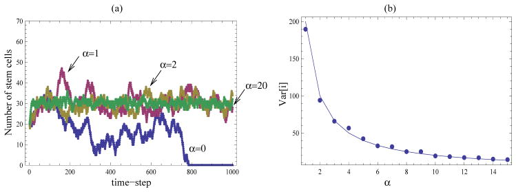
Hill-type control law. (a) Individual trajectories corresponding to the probability $p_i=\frac{i^{\alpha }}{k^{\alpha }+i^{\alpha }}$ are plotted, with k = 30, and N = 70. Different values of α are indicated in the figure. (b) The variance of the number of stem cells is computed numerically (the dots) and compared with formula (27) (solid line) for different values of α. The computations are performed for individuals runs with N = 400, k = 200, over 40, 000 time-steps.

Simplifying equations (24), we get

$$\sum _{j=0}^i\left(\begin{array}{c}i\\ j\end{array}\right){(-1)}^{i-j}{2}^{i+1-j}{x}_1^{i-j}{x}_j=0,$$ (25)

where j = α + 1, …, 2α − 1. Observe that if we treat x₁ as a constant, then the α equations (23) together with the first α − 2 equations (25) comprise a linear system with respect to variables x₂, …, x_2α−1. Solving this system allows us to represent x_i with i = 2, …, 2α−1 in terms of x₁. It is convenient to write the linear system in the matrix form,

$$M·X=B,$$

where M = (m_i,j)_{2α−2×2α−2} is the coefficient matrix, $X={(x_2,x_3,\dots ,x_{2\alpha -1})}_{1\times 2\alpha -2}^T$ is the unknown vector, and $B={(b_1,\dots ,b_{2\alpha -2})}_{1\times 2\alpha -2}^T$. We have

$$M_{ij}=\{\begin{array}{lll}\hfill \left(\begin{array}{c}i\\ j+1\end{array}\right)& ,\hfill & 1\le i\le \alpha ,1\le j\le i-2\hfill \\ \hfill \frac{1}{k^{\alpha }}\left(\begin{array}{c}i\\ j-\alpha +1\end{array}\right){(-1)}^{i-j+\alpha -1}& ,\hfill & 1\le i\le \alpha ,\alpha -1\le j\le \alpha +i-2\hfill \\ \hfill {(-1)}^{i-j-1}{2}^{i-j}{x}_1^{i-j-1}\left(\begin{array}{c}i\\ j+1\end{array}\right)& ,\hfill & \alpha +1\le i\le 2\alpha -2,1\le j\le i-1\hfill \\ \hfill 0& ,\hfill & \text{otherwise}\hfill \end{array}$$

and

$$b_i=\{\begin{array}{lll}\hfill -\frac{1}{2}& ,\hfill & i=1\hfill \\ \hfill -{ix}_1-\frac{1}{2}& ,\hfill & 2\le i\le \alpha \hfill \\ \hfill -2^i{x}_1^i({(-1)}^i+{(-1)}^{i-1}i)& ,\hfill & \alpha +1\le i\le 2\alpha -2.\hfill \end{array}$$

By using Mathematica, we can get the solution of the equation M · X = B,

$$(x_2,x_3,\dots ,x_{2\alpha -1})=(f_2(x_1),f_3(x_1),\dots ,f_{2\alpha -1}(x_1)),$$

and substitute it into the last equation (25):

$$\sum _{j=0}^{2\alpha -1}\left(\begin{array}{c}2\alpha -1\\ j\end{array}\right){(-1)}^{2\alpha -1-j}{2}^{2\alpha -j}{x}_1^{2\alpha -1-j}{x}_j=0.$$ (26)

This is a polynomial equation for x₁. Using the expansion method, where x₁ is represented as a power series in terms of k, and neglecting terms that are O(1/k), we obtain that

$$x_1=\frac{k}{2}+a,$$

where 0 < a < 1. The value of a can be found for particular values of α by using Mathematica and solving the appropriate equation set. The pattern we observe from the values α = 3, 4, 5, 6, 7 is as follows:

$$E[i]=k+\frac{1}{2\alpha }+O(1/k),\mathit{Var}[i]=\frac{k}{\alpha }+\frac{2\alpha -1}{4{\alpha }^2}+O(1/k).$$ (27)

These results are proved analytically for any α in Appendix A. Biological interpretation of these results is presented in the next section.

5 Numerical illustrations and biological interpretation

To illustrate our results, we first briefly mention the behavior of the system without control (the constant model (0)), and the system with linear control (system (1)). Figure 1 shows typical trajectories for these systems. The random walk of system (0) promptly leads to the extinction of stem cells or daughter cells (figure 1(a)), and the linear system is characterized by the standard deviation which is defined by the system size as $\sqrt{N/4}$ (figure 1(b)).

Figure 1.

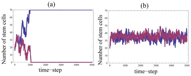
Typical trajectories corresponding to different probabilities: (a) the constant model, p_i = 0.5 and (b) the linear model, p_i = i/N, with N = 70.

In contrast to these simple examples, the hyperbolic control law contains tunable parameters which allow us to set the optimal number of the expectation for the number of stem cells, and vary its standard deviation. Figure 2(a) shows that, as predicted by formulas (7) and (9), both the expected number of the stem cells and their standard deviation are positively correlated with the control parameter, h. Although increasing h will minimize the spread, it will also decrease the expected number of stem cells. Also, increasing h may lead to the probability function defined by equation (1) outside the range [0, 1]. These considerations lead to certain constraints on the parameter h.

Figure 2.

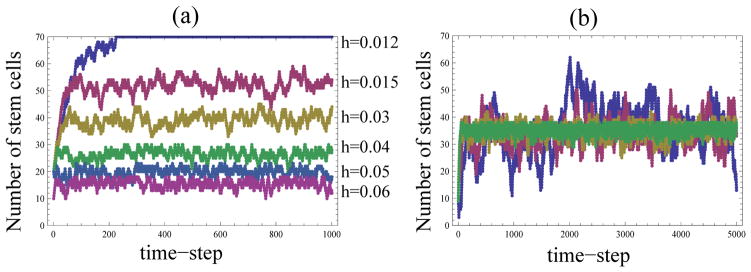
The hyperbolic law: typical runs showing the number of stem cells as a function of time. (a) The value of β is fixed to be β = 0.1, and h varies. (b) The values of β and h are given by formulas (28) and (29), with n₀ = 35 and a taking the values {3, 5, 10, 20}; the runs corresponding to larger values of a show a larger standard deviation. These are the runs that were used to calculate the means and standard deviations in figure 3(b).

Let us suppose that the system needs to maintain a certain optimal level of stem cells in the system, say n₀, and set

$$\beta =\frac{1-(n_0+1/2)h}{2}.$$ (28)

The parameter h can be varied to minimize the standard deviation. It is clear that with β given by formula (28), the variance is a monotonically decreasing function of h (figure 3(a)). Thus, increasing the amount of control will decrease the standard deviation. However, h cannot exceed the value

Figure 3.

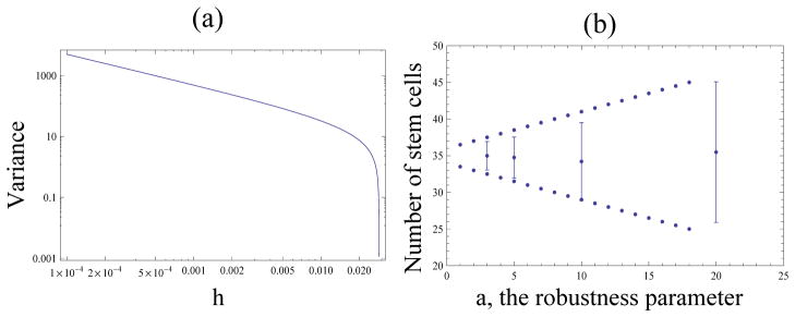
The hyperbolic law: variance as a function of control parameters. (a) Variance as a function of h for values of β given by equation (28), with n₀ = 35. (b) The numerical mean and standard deviation for the number of stem cells with β given by formula (28) with n₀ = 35 and h given by formula (29), with different values of a, the robustness parameter. The dotted lines show the theoretical estimates for the variance. The vertical bars show the standard deviations calculated from a single run, 5, 000 time-steps. The time-series of those runs are given in figure 2(b).

$$h_c={(n_0+1/2)}^{-1}$$

in order for β in equation (28) to remain positive. Therefore, the fluctuations of the number of stem cells is minimized by the values h as close as possible to h_c.

The drawback of this optimization solution is the fact that the number of stem cells can only be controlled as long as it is below n₀. If by chance it exceeds n₀, then the probability value p_i will become negative. In order to make the control solution robust, we must require that the probability p_i ∈ [0, 1] for some reasonable range of possible values of i. Let us set this requirement for the values of i within a standard deviations from the mean, $i\in \left[n_0-a\sqrt{\frac{\beta }{h}+\frac{1}{4}},n_0+a\sqrt{\frac{\beta }{h}+\frac{1}{4}}\right]$. This imposes the constraint that $h\le i_0^{-1}$, where $i_0=n_0+a\sqrt{\frac{\beta }{h}+\frac{1}{4}}$. Since higher values of h lead to smaller standard deviations, let us set $h=i_0^{-1}$, and solve this for h to obtain

$$h_{\mathit{opt}}=\frac{1}{a^2/2+n_0}.$$ (29)

This choice of the parameter h gives the standard deviation of a/2. That is, the more robust the system must be, the larger fluctuations it has to allow.

A Hill-type control mechanism allows for an independent tuning of the mean and the standard deviation of the cell population without affecting the system’s robustness, see equations (27). In particular, the parameter k must be set to the desired mean number of stem cells, and the parameter α must be increases as much as possible to minimize standard deviation. A numerical illustration is given by figure 4(a), where several typical runs corresponding to different values of α are presented. Figure 4(b) illustrates formula (27) for the variance by comparing the numerically computed variance with the theoretical prediction.

Extension to fluctuating total cell numbers

The approach used here was formulated as a Moran (constant population) process with an endogenous regulation loop controlling the proliferation/differentiation decisions of stem cells. The total population size, N, however, does not appear in the expressions for the means and the variances of stem cell populations. Therefore, the methods developed here and the results can be extended to non-constant total populations of cells.

This is demonstrated in figure 5 where we show two typical runs for a two-component system, where the numbers of stem and differentiated cells are independent stochastic variables. In figure 5(a) we assume that stem cell divisions and differentiated cell deaths are both subject to a (hyperbolic) negative control loop. Namely, at each time-step, with probability a/(1 + bN) a stem cell divides, and otherwise a differentiated cell dies, where N is the current total cell number. If a stem cell is chosen for division, then a proliferation/differentiation decision is made according to the hyperbolic law (equation (1)), exactly as in the process considered before. Figure 1(a) shows that the total population size in this process fluctuates around a quasi-steady state; the stem cells are also fluctuating around a steady state. The numerically calculated values for the mean and the variance of the stem cells are 159.4 and 20.6. These estimates are very close to the analytical predictions of formulas (7) and (9), 159.5 and 20.25 respectively.

Figure 5.

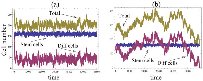
The hyperbolic law: extension to variable total populations. Typical runs showing the number of stem and differentiated cells as well as the total populations as a function of time. (a) The total number if cells is regulated endogenously by a negative control loop, where the probability for a stem cell to divide is given by a/(1+bN), where N is the total population size, a = 2.5, and b = 0.02. (b) The total number of cells fluctuates according to a symmetric Markov walk with the probability to divide given by 1/2. In both plots, the proliferation/differentiation decisions are controlled by the hyperbolic law, formula (1), with β = 0.1 and h = 0.005.

In figure 5(b) we assume a total absence of control of cell divisions and deaths. At each time step, with probability 1/2 a differentiated cell is chosen for death, and otherwise a stem cell divides. The proliferation/differentiation is assumed the same as in figure 5(a). We can see that in this case, the total number of cells follows the usual Markov walk, and the particular simulation presented here was terminated after about 60, 000 steps because the number of differentiated cells became zero. Nonetheless, the number of stem cells again oscillates around the same mean, and its mean and variance again are very close to the analytical prediction.

Results obtained for the Hill-type law are also extendable to oscillating populations (not shown). We conclude that the results obtained in this paper are valid for variable populations. Note however that an essential feature of the above models is that the regulation of proliferation/differentiation decisions is achieved through the dependence of the probability to differentiate on the number of stem cells. It does not depend directly on the number of daughter cells. In the Moran process, where the population is constant (or perhaps in a process where the total population is close to constant), this is not a problem because the number of differentiated cells is uniquely defined by the number of stem cells. In these cases we essentially have a one-dimensional process. If however the control of proliferation/differentiation decisions is achieved through a dependence on the number of differentiated cells, out modeling approach is not applicable to populations with significant fluctuations in the total population size.

6 Discussion and conclusions

In this paper we studied nonlinear mechanisms of control in stochastic dynamics of stem cells and daughter cells. The main messages of this study are formulated and discussed below.

In the absence of proliferation/differentiation control, stochastic fluctuations destroy the steady state

Stochastic systems with no control are subject to extinction/overflow even if the parameters are tuned such that the corresponding deterministic system maintains a biologically-relevant steady state. In Lander et al. (2009), a system describing stem cell/daughter cell dynamics was studied in the absence of feedback. The ordinary differential equation describing the dynamics of stem cells (x₀) and daughter cells (x₁) are given by

$${\stackrel{.}{x}}_0=(1-2p){vx}_0,$$ (30)

$${\stackrel{.}{x}}_1=2{\mathit{pvx}}_0-{dx}_1,$$ (31)

where we reduced the system used in Lander et al. (2009) to two species of cells. Here, p is the probability to differentiate, and v and d are the division and death rates respectively. Linear analysis shows that this system has a steady state only if p = 1/2. This extreme sensitivity to parameters is indicative of such a solution not being robust. Our stochastic analysis makes this point even stronger. It shows that this deterministic steady state is meaningless in the stochastic system, because it is destroyed by fluctuations, even if p = 1/2 exactly.

A tight control of death/divisions is not sufficient for tissue home-ostasis

One more conclusion that we draw from studying the system without proliferation/differentiation control is that controlling death/division decisions is not enough. In this paper we focused on the system where deaths and divisions were coupled to maintain a constant population size, which can be viewed as a limit of extremely tight death/division control. This was not sufficient to maintain a quasi-steady level of stem cells in the absence of proliferation/differentiation regulation.

Linear control is biologically implausible, as it provides no means of reducing fluctuations

Linear control mechanism, while capable of maintaining a steady population size of stem cells, contains no tunable parameters, and thus does not provide a possibility to maintain a given steady-state level of cells, and an independently controlled standard deviation.

A nonlinearity is required for robust behavior of stem cell systems, even in the simplest scenarios

We performed a stochastic analysis of two types of nonlinear control, and obtained analytical results for the stem cell statistics. Two different two-parametric control mechanisms were implemented. Despite the nonlinear form of the dependencies in the control loop, it was possible to obtain analytical expressions for the expectations and the variances of the number of stem cells.

Under the hyperbolic control law, reducing the fluctuations jeopardizes the system’s robustness

With this type of control, it is possible to tune the parameters such that a given mean number of stem cells is maintained. However, the reduction of the standard deviation leads to a compromise in the robustness of this process to external perturbations. This is an example of the well-known principle that making a system robust in one way invariably makes it fragile in another (Doyle and Csete, 2007).

The Hill-type law requires a digital (switch-type) behavior to control fluctuations

Under the Hill-type control, both the mean and the standard deviation can be controlled independently, and decreasing the size of fluctuations does not influence the system’s robustness. We find however that in order to achieve a tight control of fluctuations experienced by the population of stem and daughter cells, the value of the Hill coefficient must be relatively high. In biological terms, this corresponds to switch-like (as opposed to an analogue) behavior of the system, the so-called ultrasensitive response. In Lander et al. (2009) it was found that increasing the Hill coefficient corresponds to better performance of the deterministic system. Our stochastic analysis shows a further important advantage of the switch-like behavior: a steep control loop is optimal as it minimizes fluctuations.

Is a high Hill coefficient realistic?

As shown by our analysis, a relatively high Hill coefficient (an ultrasensitive response) can help keep the fluctuations of stem cell numbers low. A relevant biological example of a system with an autoregulatory loop is provided in a study Davey et al. (2007) where the control of embryonic stem cell self-renewal was studied. Embryonic stem cells convert leukemia inhibitory factor (LIF) concentration into an all-or-nothing cell-fate decision (self-renewal). The authors have investigated quantitatively the LIF-STAT3 dose-response profile, where the level of STAT3 is indicative of the self-renewal status. They found that the Hill coefficient is this relationship is as high as 3.0 to 4.7. Our hypothesis is that such a high Hill coefficient is an adaptation to reduce fluctuations in the system, as the steepness of the Hill function directly influences the variance of the stem cell numbers.

While many instances of ultrasensitive regulation have been described, the exact nature of the underlying biological mechanisms is still a subject of ongoing research. Several such mechanisms have been described, including zero-order effects, multisite phosphorylation, and competition mechanisms. In Meinke et al. (1986), phosphorylation of phosphorylase and isocitrate dehydrogenase in vitro has been reported, where the ultrasensitivity could be attributed to zero-order effects, which result from the kinase and/or phosphatase that regulate the steady-state level of substrate phosphorylation operating near saturation (Goldbeter and Koshland, 1981). The response of p42 MAPK to MEK may be generated by nonprocessive multisite phosphorylation (Ferrell Jr and Bhatt, 1997). The ultrasensitive response of MEK to Mos Chen et al. (1997) is explained by competition between CK2β and MEK for access to Mos. Substrate competition was shown to be the reason for ultrasensitivity in the inactivation of mitotic regulator Wee1 (Kim and Ferrell, 2007). Our hypothesis is that ultrasensitivity might have evolved as a means to reduce fluctuations and to improve the system robustness.

The models discussed here are a gross oversimplification of reality. Only two classes of cells (stem cells and daughter cells) are considered. In reality, the stem-daughter cell hierarchy can be more complicated, and cascades of differentiation should be included at the next level of model sophistication. Also, the total system size is assumed to be constant, and only differentiation decisions are regulated internally. The methods developed here are applicable to fluctuating populations if

• the biological regulation mechanism that controls the proliferation/differentiation decisions is dependent on the number of stem cells only, or

• the regulation depends on the number of differentiated cells and the total population is close to constant.

In this context, we mention that the control functions described here are not identical to those used in Lander et al. (2009); Lo et al. (2009). These authors discuss the negative control of differentiation by daughter cells. The idea is as follows. As the number of daughter cells grows, the probability for stem cells to differentiate increases such that the pool of stem cells decreases, leading to a subsequent decrease in the number of daughter cells. The control loops in Lander et al. (2009); Lo et al. (2009) regulate the dynamics of stem cells by changing p as a decreasing function of the number of daughter cells. This is equivalent to the function p in our models being a decreasing function of the number of differentiated cells. In the present paper, the function p is an increasing function of the number of stem cells, which in general is a very different biological mechanism. If we assume that the total number of stem and daughter cells is (nearly) constant, then two types of regulation are mathematically equivalent. In systems without this restriction, or in systems with multistage cell lineages, the two mechanisms would be different. A system where both division and differentiation decisions are subject to internal control loops, and differentiation is controlled by the number of differentiated cells, is investigated elsewhere (Sun and Komarova, 2012). Analysis of more biologically realistic systems with positive and negative control loops is a subject of current and future work.

• We study stochastic regulation of stem-cell renewall.

• Stochastic systems with no control are subject to extinction/overflow.

• Analytical solutions for mean and variance with nonlinear control are found.

• For hyperbolic control, there is a trade-off between fluctuations and robustness.

• For Hill-type control, fluctuations are inversely proportional to the Hill coefficient.

A The Hill-type law: the case of a general α

In this section, we to prove the following results analytically:

$$E[i]=k+\frac{1}{2\alpha }+O(1/k),\mathit{Var}[i]=\frac{k}{\alpha }+\frac{2\alpha -1}{4{\alpha }^2}+O(1/k).$$ (32)

By formulas (16) and (18),

$$E[i]=2x_1+\frac{1}{2},\mathit{Var}[i]=2x_2-4x_1^2+\frac{1}{4}.$$

Therefore,

$$\begin{array}{c}E[i]=k+O(1)\iff x_1=k/2+a+O(k^{-1}),\\ \mathit{Var}[i]=\frac{k}{\alpha }+O(1)\iff 2x_2-4{(\frac{k}{2}+a)}^2+\frac{1}{4}+O(1)=\frac{k}{\alpha }+O(1),\end{array}$$

which means that

$$x_2=\frac{k^2}{2}+\frac{1}{2}(\frac{1}{\alpha }+4a)k+O(1)$$

for some constant a in ℜ. Therefore, in order to prove formula (32), we only need to prove that

$$\{\begin{array}{l}{x}_1=\frac{k}{2}+a+O(k^{-1})\hfill \\ x_2=\frac{k^2}{2}+\frac{1}{2}(\frac{1}{\alpha }+4a)k+O(1)\hfill \end{array}$$ (33)

for some constant a. Performing calculations for individual cases of α, and looking for patterns in the expressions for x₂, we observe that

$$x_2=\frac{k^2}{2}-\frac{\alpha -2}{2\alpha }k.$$ (34)

Comparing formulas (33) and (34), we get

$$\begin{array}{c}\frac{1}{2}(\frac{1}{\alpha }+4a)=-\frac{\alpha -2}{2\alpha }\\ \Rightarrow a=\frac{1-\alpha }{4\alpha }.\end{array}$$

Substituting a in formula (33), we get

$$x_1=\frac{k}{2}+\frac{1-\alpha }{4\alpha }.$$

Therefore, we only need to prove that

$$\{\begin{array}{l}{x}_1=\frac{k}{2}+\frac{1-\alpha }{4\alpha }\hfill \\ x_2=\frac{k^2}{2}+\frac{2-\alpha }{2\alpha }k.\hfill \end{array}$$ (35)

After observing several specific cases, we claim that the solution for x₁, x₂, …, x_2α−1 has the following form:

$$x_{\gamma }=\frac{k^{\gamma }}{2}+\frac{{\gamma }^2-\gamma \alpha }{4\alpha }{k}^{\gamma -1},$$ (36)

where $1\le \gamma \le \lfloor \frac{\alpha }{2}\rfloor$, and

$$x_{\gamma }=x_{\alpha -\gamma }{k}^{2\gamma -\alpha },$$ (37)

where $\lfloor \frac{\alpha }{2}\rfloor +1\le \gamma \le \alpha -1$. If we only consider the first two highest order terms with respect to k in equation (23), we get

$$x_{\alpha +\gamma }=\frac{\gamma }{2}{k}^{\alpha +\gamma -1}+k^{\alpha }{x}_{\gamma },$$ (38)

where 1 ≤ γ ≤ α − 1. Substituting expressions (36) and (37) in equation (38), we obtain formulas for x_α+γ, where 0 ≤ γ ≤ α − 1. In particular, we have

$$x_{\alpha +\gamma }=\frac{k^{\alpha +\gamma }}{2}+\frac{{\gamma }^2+\gamma \alpha }{4\alpha }{k}^{\alpha +\gamma -1},0\le \gamma \le \lfloor \frac{\alpha }{2}\rfloor ,$$ (39)

and

$$x_{\alpha +\gamma }=\frac{k^{\alpha +\gamma }}{2}+\frac{2{\alpha }^2-3(\alpha -\gamma )\alpha +{(\alpha -\gamma )}^2}{4\alpha }{k}^{\alpha +\gamma -1},\lfloor \frac{\alpha }{2}\rfloor +1\le \gamma \le \alpha -1.$$ (40)

In the above expression, we only need to consider the first and the second highest order terms with respect to k.

We claim that expressions (36), (37), (39), and (40) are approximate (in terms of k) solutions for equations (23, 25). To show this it is enough to demonstrate that in equation (25), terms of the two highest in k orders vanish. Equation (25) is becomes

$$\sum _{j=0}^{\alpha +\gamma }\left(\begin{array}{c}\alpha +\gamma \\ j\end{array}\right){(-1)}^{\alpha +\gamma -j}{2}^{\alpha +\gamma -j}{x}_1^{\alpha +\gamma -j}{x}_j=0,$$

where γ = 1, 2, …, α − 1. After simplification, we can get the following formula for the terms $x_1^{\alpha +\gamma -j}{x}_j$ with γ = 1, 2, …, α − 1:

$$x_1^{\alpha +\gamma -j}{x}_j=\{\begin{array}{lll}{(\frac{1}{2})}^{\alpha +\gamma +1-j}{k}^{\alpha +\gamma }+{(\frac{1}{2})}^{\alpha +\gamma -j}\frac{j^2-j+(\gamma +\alpha )(1-\alpha )}{4\alpha }{k}^{\alpha +\gamma -1}\hfill & ,\hfill & 0\le j\le \alpha -1\hfill \\ {(\frac{1}{2})}^{\gamma -m+1}{k}^{\alpha +\gamma }+{(\frac{1}{2})}^{\gamma -m}\frac{m^2+m\alpha +(\gamma -m)(1-\alpha )}{4\alpha }{k}^{\alpha +\gamma -1}\hfill & ,\hfill & 0\le m\le \gamma ,(m=j-\alpha )\hfill \end{array}$$ (41)

The coefficient in front of the highest order term, k^α+γ, is

$$\begin{array}{l}{c}_{\alpha +\gamma }=\sum _{j=0}^{\alpha +\gamma }{(\frac{1}{2})}^{\alpha +\gamma +1-j}\left(\begin{array}{c}\alpha +\gamma \\ j\end{array}\right){(-1)}^{\alpha +\gamma -j}{2}^{\alpha +\gamma -j}\\ =\frac{1}{2}\sum _{j=0}^{\alpha +\gamma }\left(\begin{array}{c}\alpha +\gamma \\ j\end{array}\right){(-1)}^{\alpha +\gamma -j}\\ =\frac{1}{2}{(1-1)}^{\alpha +\gamma }=0.\end{array}$$

Next, we prove that the the second highest order term is also 0. The coefficient in front of k^α+γ−1 is

$$\begin{array}{l}{c}_{\alpha +\gamma -1}=\sum _{j=0}^{\alpha -1}\left(\begin{array}{c}\alpha +\gamma \\ j\end{array}\right){(-1)}^{\alpha +\gamma -j}\frac{j^2-j+(\gamma +\alpha )(1-\alpha )}{4\alpha }+\sum _{m=0}^{\gamma }\frac{m^2+m\alpha +(\gamma -m)(1-\alpha )}{4\alpha }\left(\begin{array}{c}\alpha +\gamma \\ \alpha +m\end{array}\right){(-1)}^{\gamma -m}\\ =\sum _{j=0}^{\alpha -1}\left(\begin{array}{c}\alpha +\gamma \\ j\end{array}\right){(-1)}^{\alpha +\gamma -j}\frac{j^2-j}{4\alpha }+\sum _{j=0}^{\alpha -1}\left(\begin{array}{c}\alpha +\gamma \\ j\end{array}\right){(-1)}^{\alpha +\gamma -j}\frac{(\gamma +\alpha )(1-\alpha )}{4\alpha }+\sum _{m=0}^{\gamma }\frac{m^2+m\alpha }{4\alpha }\left(\begin{array}{c}\alpha +\gamma \\ \alpha +m\end{array}\right){(-1)}^{\gamma -m}+\sum _{m=0}^{\gamma }\frac{(\gamma -m)(1-\alpha )}{4\alpha }\left(\begin{array}{c}\alpha +\gamma \\ \alpha +m\end{array}\right){(-1)}^{\gamma -m}.\end{array}$$

Let A, B, C, D denote the four terms in the last equation. Simplifying A, B, C, and D, we get

$$\begin{array}{l}A=\sum _{j=2}^{\alpha -1}\left(\begin{array}{c}\alpha +\gamma \\ j\end{array}\right){(-1)}^{\alpha +\gamma -j}\frac{j(j-1)}{4\alpha }\\ =\frac{1}{4\alpha }\sum _{j=2}^{\alpha -1}{(-1)}^{\alpha +\gamma -j}\left(\begin{array}{c}\alpha +\gamma -2\\ j-2\end{array}\right)(\alpha +\gamma )(\alpha +\gamma -1)\\ =\frac{(\alpha +\gamma )(\alpha +\gamma -1)}{4\alpha }\sum _{j=2}^{\alpha -1}{(-1)}^{\alpha +\gamma -j}\left(\begin{array}{c}\alpha +\gamma -2\\ j-2\end{array}\right).\\ B=\frac{(\gamma +\alpha )(1-\alpha )}{4\alpha }[\sum _{j=0}^{\alpha -1}\left(\begin{array}{c}\alpha +\gamma \\ j\end{array}\right){(-1)}^{\alpha +\gamma -j}+\sum _{j=\alpha }^{\alpha +\gamma }\left(\begin{array}{c}\alpha +\gamma \\ j\end{array}\right){(-1)}^{\alpha +\gamma -j}-\sum _{j=\alpha }^{\alpha +\gamma }\left(\begin{array}{c}\alpha +\gamma \\ j\end{array}\right){(-1)}^{\alpha +\gamma -j}]\\ =\frac{(\gamma +\alpha )(1-\alpha )}{4\alpha }{(1-1)}^{\alpha +\gamma }-\frac{(\gamma +\alpha )(1-\alpha )}{4\alpha }\sum _{j=\alpha }^{\alpha +\gamma }\left(\begin{array}{c}\alpha +\gamma \\ j\end{array}\right){(-1)}^{\alpha +\gamma -j}\\ =-\frac{(\gamma +\alpha )(1-\alpha )}{4\alpha }\sum _{j=\alpha }^{\alpha +\gamma }\left(\begin{array}{c}\alpha +\gamma \\ j\end{array}\right){(-1)}^{\alpha +\gamma -j}.\\ C=\sum _{m=0}^{\gamma }\frac{m^2+m\alpha }{4\alpha }\left(\begin{array}{c}\alpha +\gamma \\ \alpha +m\end{array}\right){(-1)}^{\gamma -m}\\ =\sum _{j=\alpha }^{\alpha +\gamma }\frac{{(j-\alpha )}^2-\alpha (j-\alpha )}{4\alpha }\left(\begin{array}{c}\alpha +\gamma \\ j\end{array}\right){(-1)}^{\alpha +\gamma -j}\\ =\sum _{j=\alpha }^{\alpha +\gamma }\frac{j^2-\alpha j}{4\alpha }\left(\begin{array}{c}\alpha +\gamma \\ j\end{array}\right){(-1)}^{\alpha +\gamma -j}.\end{array}$$

In the expression above we let m = j − α. Finally,

$$D=\sum _{j=\alpha }^{\alpha +\gamma }\frac{(\gamma -j+\alpha )(1-\alpha )}{4\alpha }\left(\begin{array}{c}\alpha +\gamma \\ j\end{array}\right){(-1)}^{\alpha +\gamma -j}.$$

Using these expressions, we find

$$\begin{array}{l}B+D=\sum _{j=\alpha }^{\alpha +\gamma }\left(\begin{array}{c}\alpha +\gamma \\ j\end{array}\right){(-1)}^{\alpha +\gamma -j}\frac{1}{4\alpha }((\gamma -j+\alpha )(1-\alpha )-(\gamma +\alpha )(1-\alpha ))\\ =\frac{1}{4\alpha }\sum _{j=\alpha }^{\alpha +\gamma }\left(\begin{array}{c}\alpha +\gamma \\ j\end{array}\right){(-1)}^{\alpha +\gamma -j}(-j+j\alpha ),\\ C+B+D=\frac{1}{4\alpha }\sum _{j=\alpha }^{\alpha +\gamma }\left(\begin{array}{c}\alpha +\gamma \\ j\end{array}\right){(-1)}^{\alpha +\gamma -j}(j^2-j)\\ =\frac{(\alpha +\gamma )(\alpha +\gamma -1)}{4\alpha }\sum _{j=\alpha }^{\alpha +\gamma }{(-1)}^{\alpha +\gamma -j}\left(\begin{array}{c}\alpha +\gamma -2\\ j-2\end{array}\right),\\ A+B+C+D=\frac{(\alpha +\gamma )(\alpha +\gamma -1)}{4\alpha }\sum _{j=2}^{\alpha +\gamma }{(-1)}^{\alpha +\gamma -j}\left(\begin{array}{c}\alpha +\gamma -2\\ j-2\end{array}\right)\\ =\frac{(\alpha +\gamma )(\alpha +\gamma -1)}{4\alpha }\sum _{m=0}^{\alpha +\gamma -2}\left(\begin{array}{c}\alpha +\gamma -2\\ m\end{array}\right){(-1)}^{\alpha +\gamma -m}\\ =\frac{(\alpha +\gamma )(\alpha +\gamma -1)}{4\alpha }{(1-1)}^{\alpha +\gamma -2}=0,\end{array}$$

where m = j − 2.

We have proved that the coefficient in front of k^α+γ−1, which is given by A + B + C + D, is identically zero. Therefore expressions (36), (37), (39), (40) are indeed solutions of equation system (23,25). Therefore, expressions (32 hold true.

B Cumulant closure method for the Hill-type law

In this appendix we demonstrate how the cumulant closure method can be used to study the mean and the variance for the Hill law model with α = 3. By using the same notations as before, first we obtain three equations about the moments x₁, x₂, x₃, x₄, x₅, where x_k = Σf_ii^k:

$$x_3=\frac{k^3}{2}$$ (42)

$$2x_1-2\frac{x_4}{k^3}+1=0$$ (43)

$$x_2-\frac{x_5}{k^3}+2x_1+\frac{1}{2}=0$$ (44)

This is not a closed system. We will use the cumulant closure method to find the solution for x_i. Namely, we add two more equations,

$${\kappa }_4=0,$$ (45)

$${\kappa }_5=0,$$ (46)

where κ₄ and κ₅ are cumulants for the 4th and 5th order. By definition of the cumulant, we know that

$${\kappa }_4={\mu }_4-4{\mu }_3{\mu }_1-3{\mu }_2^2+12{\mu }_2{\mu }_1^2-6{\mu }_1^4,$$ (47)

$${\kappa }_5={\mu }_5-5{\mu }_4{\mu }_1-10{\mu }_3{\mu }_2+20{\mu }_3{\mu }_1^2+30{\mu }_2^2{\mu }_1-60{\mu }_2{\mu }_1^3+24{\mu }_1^5,$$ (48)

where quantities μ_i are the raw moments for the distribution {f̂_i} = {2f_i}. Using μ_i = 2x_i and substituting in equations (47) and (48), we obtain two equations for x_i,

$$-48x_1^4+48x_1^2{x}_2-6x_2^2-8x_1{x}_3+x_4=0,$$ (49)

$$384x_1^5-480x_1^3{x}_2+120x_1{x}_2^2+80x_1^2{x}_3-20x_2{x}_3-10x_1{x}_4+x_5=0.$$ (50)

As before, we assume that x₁ = a₁k + a₂, and solve the equations for each order in k. We obtain

$$x_1=\frac{k}{2}-\frac{1}{6}.$$

Therefore,

$$E[i]=k+\frac{1}{6},$$ (51)

$$\mathit{Var}[i]=\frac{k}{3}+\frac{7}{36}.$$ (52)

References

- Adimy M, Crauste F, Ruan S. Bull Math Biol. 2006;68:2321. doi: 10.1007/s11538-006-9121-9. [DOI] [PubMed] [Google Scholar]
- Agur Z, Daniel Y, Ginosar Y. Journal of mathematical biology. 2002;44(1):79. doi: 10.1007/s002850100115. [DOI] [PubMed] [Google Scholar]
- Binetruy B, Heasley L, Bost F, Caron L, Aouadi M. Stem Cells. 2007;25:1090. doi: 10.1634/stemcells.2006-0612. [DOI] [PubMed] [Google Scholar]
- Boman BM, Fields JZ, Cavanaugh KL, Guetter A, Runquist OA. Cancer Res. 2008;68:3304. doi: 10.1158/0008-5472.CAN-07-2061. [DOI] [PubMed] [Google Scholar]
- Chen M, Li D, Krebs E, Cooper J. Molecular and cellular biology. 1997;17(4):1904. doi: 10.1128/mcb.17.4.1904. [DOI] [PMC free article] [PubMed] [Google Scholar]
- Close J, Gumuscu B, Reh T. Development. 2005;132(13):3015. doi: 10.1242/dev.01882. [DOI] [PubMed] [Google Scholar]
- Colijn C, Mackey MC. J Theor Biol. 2005;237:117. doi: 10.1016/j.jtbi.2005.03.033. [DOI] [PubMed] [Google Scholar]
- Daluiski A, Engstrand T, Bahamonde M, Gamer L, Agius E, Stevenson S, Cox K, Rosen V, Lyons K. Nature genetics. 2001;27(1):84. doi: 10.1038/83810. [DOI] [PubMed] [Google Scholar]
- Davey R, Onishi K, Mahdavi A, Zandstra P. The FASEB Journal. 2007;21(9):2020. doi: 10.1096/fj.06-7852com. [DOI] [PubMed] [Google Scholar]
- Discher DE, Mooney DJ, Zandstra PW. Science. 2009;324:1673. doi: 10.1126/science.1171643. [DOI] [PMC free article] [PubMed] [Google Scholar]
- d’Onofrio A, Tomlinson IP. J Theor Biol. 2007;244:367. doi: 10.1016/j.jtbi.2006.08.022. [DOI] [PubMed] [Google Scholar]
- Doyle J, Csete M. Nature. 2007;446(7138):860. doi: 10.1038/446860a. [DOI] [PubMed] [Google Scholar]
- Endo D, Maku-Uchi M, Kojima I. Endocrine journal. 2006;53(1):73. doi: 10.1507/endocrj.53.73. [DOI] [PubMed] [Google Scholar]
- Ferrell JE. Bioessays. 1999;21:866. doi: 10.1002/(SICI)1521-1878(199910)21:10<866::AID-BIES9>3.0.CO;2-1. [DOI] [PubMed] [Google Scholar]
- Ferrell J, Jr, Bhatt R. Journal of Biological Chemistry. 1997;272(30):19008. doi: 10.1074/jbc.272.30.19008. [DOI] [PubMed] [Google Scholar]
- Gan Q, Yoshida T, McDonald OG, Owens GK. Stem Cells. 2007;25:2. doi: 10.1634/stemcells.2006-0383. [DOI] [PubMed] [Google Scholar]
- Glauche I, Cross M, Loeffler M, Roeder I. Stem Cells. 2007;25:1791. doi: 10.1634/stemcells.2007-0025. [DOI] [PubMed] [Google Scholar]
- Goldbeter A, Koshland DE. Proc Natl Acad Sci USA. 1981;78:6840. doi: 10.1073/pnas.78.11.6840. [DOI] [PMC free article] [PubMed] [Google Scholar]
- Hardy K, Stark J. Apoptosis. 2002;7:373. doi: 10.1023/a:1016183731694. [DOI] [PubMed] [Google Scholar]
- Iwasa Y, Michor F, Komarova N, Nowak M. Journal of theoretical biology. 2005;233(1):15. doi: 10.1016/j.jtbi.2004.09.001. [DOI] [PubMed] [Google Scholar]
- Johnston MD, Edwards CM, Bodmer WF, Maini PK, Chapman SJ. Proc Natl Acad Sci USA. 2007;104:4008. doi: 10.1073/pnas.0611179104. [DOI] [PMC free article] [PubMed] [Google Scholar]
- Khammash M. BioTechniques. 2008;44:323. doi: 10.2144/000112772. [DOI] [PubMed] [Google Scholar]
- Kim SY, Ferrell JE. Cell. 2007;128:1133. doi: 10.1016/j.cell.2007.01.039. [DOI] [PubMed] [Google Scholar]
- Komarova N. Bulletin of mathematical biology. 2006;68(7):1573. doi: 10.1007/s11538-005-9046-8. [DOI] [PubMed] [Google Scholar]
- Komarova N, Sengupta A, Nowak M. Journal of theoretical biology. 2003;223(4):433. doi: 10.1016/s0022-5193(03)00120-6. [DOI] [PubMed] [Google Scholar]
- Lander A. Cell. 2011;144(6):955. doi: 10.1016/j.cell.2011.03.009. [DOI] [PMC free article] [PubMed] [Google Scholar]
- Lander AD, Gokoffski KK, Wan FY, Nie Q, Calof AL. PLoS Biol. 2009;7:e15. doi: 10.1371/journal.pbio.1000015. [DOI] [PMC free article] [PubMed] [Google Scholar]
- Lee CH, Kim KH, Kim P. J Chem Phys. 2009;130:134107. doi: 10.1063/1.3103264. [DOI] [PubMed] [Google Scholar]
- Lieberman E, Hauert C, Nowak M. Nature. 2005;433(7023):312. doi: 10.1038/nature03204. [DOI] [PubMed] [Google Scholar]
- Lloyd AL. Theor Popul Biol. 2004;65:49. doi: 10.1016/j.tpb.2003.07.002. [DOI] [PubMed] [Google Scholar]
- Lo WC, Chou CS, Gokoffski KK, Wan FY, Lander AD, Calof AL, Nie Q. Math Biosci Eng. 2009;6:59. doi: 10.3934/mbe.2009.6.59. [DOI] [PMC free article] [PubMed] [Google Scholar]
- Loeffler M, Roeder I. Cells Tissues Organs (Print) 2002;171:8. doi: 10.1159/000057688. [DOI] [PubMed] [Google Scholar]
- MacKey MC. Cell Prolif. 2001;34:71. doi: 10.1046/j.1365-2184.2001.00195.x. [DOI] [PMC free article] [PubMed] [Google Scholar]
- Mangel M, Bonsall MB. PLoS ONE. 2008;3:e1591. doi: 10.1371/journal.pone.0001591. [DOI] [PMC free article] [PubMed] [Google Scholar]
- Marshall E, Lord B. International review of cytology. 1996;167:185. doi: 10.1016/s0074-7696(08)61348-0. [DOI] [PubMed] [Google Scholar]
- Meinke M, Bishop J, Edstrom R. Proceedings of the National Academy of Sciences. 1986;83(9):2865. doi: 10.1073/pnas.83.9.2865. [DOI] [PMC free article] [PubMed] [Google Scholar]
- Moran PAP. The Statistical Process of Evolutionary Theory. Oxford: Clarendon Press; 1962. [Google Scholar]
- Murray J. Mathematical Biology I: An Introdauction. New York: Springer; 2002. [Google Scholar]
- Nasell I. Theor Popul Biol. 2003;63:159. doi: 10.1016/s0040-5809(02)00060-6. [DOI] [PubMed] [Google Scholar]
- Novak B, Tyson JJ. Biochem Soc Trans. 2003;31:1526. doi: 10.1042/bst0311526. [DOI] [PubMed] [Google Scholar]
- Platel J, Dave K, Bordey A. The Journal of physiology. 2008;586(16):3739. doi: 10.1113/jphysiol.2008.155325. [DOI] [PMC free article] [PubMed] [Google Scholar]
- Plikus M, Mayer J, de La Cruz D, Baker R, Maini P, Maxson R, Chuong C. Nature. 2008;451(7176):340. doi: 10.1038/nature06457. [DOI] [PMC free article] [PubMed] [Google Scholar]
- Richardson J. Symp Appl Math. 1964;16:290. [Google Scholar]
- Singh A, Hespanha JP. Bull Math Biol. 2007;69:1909. doi: 10.1007/s11538-007-9198-9. [DOI] [PubMed] [Google Scholar]
- Socha L. Linearization methods for stochastic dynamic systems. Berlin: Springer; 2008. [Google Scholar]
- Sun Z, Komarova N. 2012 Submitted. [Google Scholar]
- Thalhauser C, Lowengrub J, Stupack D, Komarova N. 2010:1–17. doi: 10.1186/1745-6150-5-21. [DOI] [PMC free article] [PubMed] [Google Scholar]
- Tomlinson IP, Bodmer WF. Proc Natl Acad Sci USA. 1995;92:11130. doi: 10.1073/pnas.92.24.11130. [DOI] [PMC free article] [PubMed] [Google Scholar]
- Tothova Z, Gilliland DG. Cell Stem Cell. 2007;1:140. doi: 10.1016/j.stem.2007.07.017. [DOI] [PubMed] [Google Scholar]
- Traulsen A, Claussen J, Hauert C. Physical review letters. 2005;95(23):238701. doi: 10.1103/PhysRevLett.95.238701. [DOI] [PubMed] [Google Scholar]
- Traulsen A, Pacheco J, Dingli D. Stem Cells. 2007;25(12):3081. doi: 10.1634/stemcells.2007-0427. [DOI] [PubMed] [Google Scholar]
- Tsankov AM, Brown CR, Yu MC, Win MZ, Silver PA, Casolari JM. Mol Syst Biol. 2006;2:65. doi: 10.1038/msb4100106. [DOI] [PMC free article] [PubMed] [Google Scholar]
- Tyson JJ, Chen KC, Novak B. Curr Opin Cell Biol. 2003;15:221. doi: 10.1016/s0955-0674(03)00017-6. [DOI] [PubMed] [Google Scholar]
- Wu H, Ivkovic S, Murray R, Jaramillo S, Lyons K, Johnson J, Calof A. Neuron. 2003;37(2):197. doi: 10.1016/s0896-6273(02)01172-8. [DOI] [PubMed] [Google Scholar]
- Yamasaki K, Toriu N, Hanakawa Y, Shirakata Y, Sayama K, Takayanagi A, Ohtsubo M, Gamou S, Shimizu N, Fujii M, et al. Journal of investigative dermatology. 2003;120(6):1030. doi: 10.1046/j.1523-1747.2003.12239.x. [DOI] [PubMed] [Google Scholar]
- Yatabe Y, Tavare S, Shibata D. Proc Natl Acad Sci USA. 2001;98:10839. doi: 10.1073/pnas.191225998. [DOI] [PMC free article] [PubMed] [Google Scholar]