SUMMARY
Protein turnover studies on a proteome scale based on metabolic isotopic labeling can provide a systematic understanding of mechanisms for regulation of protein abundances and their transient behaviors. At this time, these large-scale studies typically utilize a simple kinetic model to extract protein dynamic information. Although many high quality, protein isotope incorporation data are available from those experiments, accurate and additionally useful protein dynamic information cannot be extracted from the experimental data by use the simple kinetic models. In this paper, we describe a formal connection between data obtained from elemental isotope labeling experiments and the well-known compartment modeling, and demonstrate that an appropriate application of a compartment model to turnover of proteins from mammalian tissue can indeed lead to a better fitting of the experimental data.
INTRODUCTION
Quantitative proteomics studies typically provide static comparison of protein abundance differences of the system under study. However, proteins are constantly synthesized and degraded in a living organism depending on their cellular localization and functionality even if their concentrations are kept constant. Although proteins are synthesized by a canonical pathway, protein synthesis rates are subjected to precise transcriptional and translational controls, and influenced by the availability of amino acids. A cell also possesses a number of pathways to remove unwanted protein from the system to modulate the appropriate protein abundances. Abnormal activities of protein degradation pathways have been associated with the onset of numerous diseases. It is likely that all neurodegenerative disorders, including Alzheimer’s (AD), Parkinson’s, and Huntington’s diseases as well as the frontotemporal dementias, may result from the inability of cells to remove the prion forms of etiologic proteins, which subsequently assemble into insoluble aggregates1. Understanding the molecular mechanisms of those neurodegenerative diseases may be facilitated by direct measurement of protein turnover in healthy and diseased tissues.
To study protein turnover, it is necessary to apply metabolic isotope labeling methods to trace the amino acid incorporation into a protein. For single-cell organisms, dynamic stable isotope labeling in culture (dynamic SILAC) experiments2–4 utilize a single or a few isotopically labeled amino acids to measure protein turnover on a proteome scale. The abundance ratio of labeled and unlabeled peptide ions can be directly used to construct peptide incorporation curves. The free amino acid cytosolic pool in cell cultures can be primed readily with the isotope labels by changing the growth media and the unlabeled amino acids produced by degradation can be quickly diffused into the labeled media. The protein turnover kinetics typically follows a simple exponential mechanism. It is expected that protein turnover in a complex organism, such as a mammal, has much more complicated kinetics.
Recently, we have traced the global protein turnover in mammalian tissues by use of 15N stable isotope labeling and high resolution mass spectrometry detection5. Unlike typical dynamic SILAC experiments, all nitrogen atoms in the food source are labeled with the heavy nitrogen isotope. The advantages of using 15N labeling include easy production of a natural food source (blue-green algae; Spirulina platensis) for mammalian models with near purity of heavy isotope and high dynamic range of isotope incorporation measurement. A disadvantage of the single-element labeling compared to the single amino-acid labeling is that more sophisticated data processing software is needed to extract protein turnover information from complex spectra containing many isotopic peaks. A data processing platform that fulfills this requirement has been described elsewhere6. Using a combination of careful execution of optimized experimental protocols and robust data processing algorithms, we were able to measure protein turnover rate constants for ~1700 proteins in mouse tissues. In order to obtain global proteome dynamics in the mammalian samples, we used a simple empirical kinetic model to capture the essence of protein turnover in different tissues. A delayed exponential function was proposed to describe the simple kinetic model7. The delay time parameter was included to account for the delay in delivering amino acids from the digestion of the food source. Although the simple kinetic model or the simple model functional form of amino acid incorporation curve fits the general structure of the peptide/protein incorporation curves, there are discrepancies in details of the experimental data so that the simple functional form cannot fit well. In this contribution, we describe the use of more sophisticated compartment kinetic models in an attempt to explain the observed discrepancies. Although the concept of compartment modeling for protein turnover was developed in 1950s8, 9, we have not found adequate literature providing a clear description for its applications to large-scale dynamic proteomics studies. Here, we attempt to establish a consistent relationship between the experimentally observed data with a compartment model with minimal parameters. The newly developed compartment models can provide the functional forms that can be used for more satisfactory fitting to experimentally observed protein incorporation curves, compared to the simple, widely used one-exponential function.
THEORY
One-compartment model
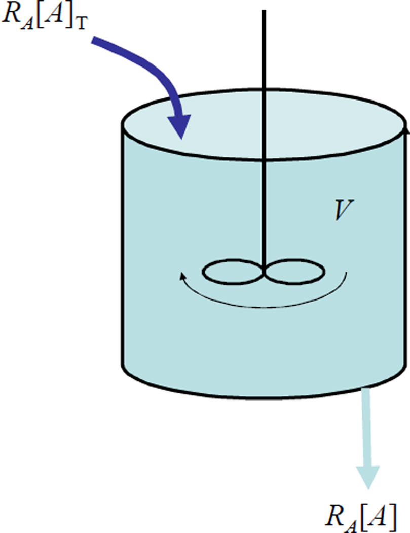
Before examining compartment models for isotope labeling of proteins, we investigated the kinetic information that can be extracted from compartment modeling by measuring relative concentration of labels (Figure 1). In the one-compartment model shown in Figure 1, let RA be the flow rate of pure label A into a compartment (or a pool) initially containing no label, with a volume of V, starting at t=0. There are two key assumptions of our current compartment modeling. The first assumption is that a label mixes instantly in a compartment. The second assumption is the size of a compartment does not change during the experiment. In the model, the same volume of mixed material must flow out of the compartment. The concentration of label, [A], in the compartment can be described by the differential equation
| (1) |
in which [A]T is the concentration of pure label A. If we measure the relative concentration of A in the compartment, the above equation becomes
| (2) |
in which is the relative (or fractional) concentration of label A. The solution of the equation is
| (3) |
Therefore, the rate constant, , is the relative volumetric flow rate of label A and the rate constant is inversely proportional to the size of the compartment. This derivation highlights a limitation of an experiment based on measurement of relative concentration of labels. Independent experiments must be carried out in order to obtain independent information about mass or volumetric flow rates or the sizes of compartments.
Figure 1.
One-compartment model. RA[A]T and RA[A] are the quantities (moles if the concentrations are in Molar unit and RA is in liter per unit time) flowed into and out of the compartment per unit of time, respectively.
Two-compartment model of isotope labeling
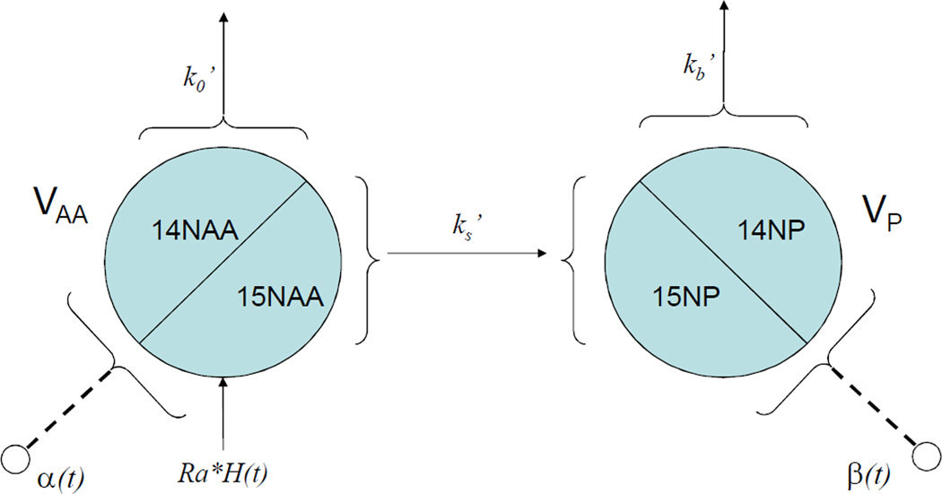
We now consider 15N-labeled amino acids in a two-compartment model (Figure 2). We assign
[AA] as the total concentration of amino acids in the free amino acid pool,
[P] as the total concentration of amino acid in the protein-bound pool,
VAA as the volumetric size of the free amino acid pool,
VP as the volumetric size of the protein-bound pool,
[14NAA] as the concentration of 14N amino acid in the free amino acid pool,
[15NAA] as the concentration of 15N amino acid in the free amino acid pool,
[14NP] as the concentration of 14N amino acid in the protein-bound pool, and
[15NP] as the concentration of 15N amino acid in the protein-bound pool.
Figure 2.
Two-compartment model for protein turnover in brain. H(t) is the step function of t; H(t)=0 for t<0 and H(t)=1 for t>=0. VAA and VP are the volumetric sizes of the free amino acid pool and the protein-bound pool, respectively. Assuming there is not an isotope effect, the rate constants are the same for both unlabeled and labeled amino acids. α and β are the fractional concentration of 15N-labeled amino acids in the free amino acid pool and the protein-bound pool, respectively.
The model neglects the contribution of the breakdown of a protein of interest into the free amino acid pool because an individual protein’s contribution is likely to be small. Assume at time t=0, 14N food source is replaced by 15N food source with constant amino acid influx of Ra. According to the model, the following equations can be established for 14N amino acid
| (4) |
| (5) |
and for 15N amino acid
| (6) |
| (7) |
Under a homeostatic condition (compartment sizes are constant), the total concentration of the free amino acid pool [AA] and that for the protein-bound pool [P] are constants
| (8) |
| (9) |
We can derive the following relationship due to mass conservation
| (10) |
by use of Equations 4 and 6 and
| (11) |
by use of Equations 5 and 7. The differential equations 4–7 are also subjected to the initial conditions (the experimental procedure)
| (12) |
| (13) |
Equations 5 and 7 can be combined to give introduction of the following variables
| (14) |
| (15) |
and transforms Equations 6 and 7 into
| (16) |
| (17) |
with the initial conditions of
| (18) |
| (19) |
in which is the lumped rate constant for amino acid removal from the free amino acid pool and is the protein degradation rate constant. Just as illustrated in the one-compartment model, it is clear that those rate constants are the relative volumetric flow rate constants normalized by their respective compartment volume sizes. The solution of Equation 16 is an exponential decay function and the solution of Equation 17 is that driven by the exponential decay. Equations 16–17 can be easily solved by use of Laplace transform and the solution of interest as
| (20) |
| (21) |
The half-life times for the free amino acid pool and the protein pool can be found as ln(2) / k0 and ln(2) / kb, respectively. Depending on the compartment model and where the label concentrations are measured, some parameters cannot be uniquely determined. The investigation of whether parameters can be determined is called identifiability analysis8. In this model, we should be able to extract protein degradation and free amino acid removal rate constants by measuring the amino acid relative concentration in the protein-bound pool alone (β).
Relationship between compartment models and experimental data
Now, we need to establish a connection between the relative 15N-labeled amino acid concentration in protein (β, Equation 15) and the experimentally observed data. Each amino acid contains at least one nitrogen atom; some amino acids contain two (asparagine, glutamine, lysine, and tryptophan), three (histidine), or four (arginine) nitrogen atoms. The relative concentration of 15N-labeled amino acid in a peptide is proportional to the relative concentration of 15N atoms in the peptide if all amino acids incorporate into proteins with the same probability. This is, of course, an approximation because there is some delay for non-essential amino acids to become available compared to the essential amino acids. The proportional constant is 1.3577 for an averagine10. The proportional constant cancels out when computing the relative fractional concentration (Equation 15). In our data processing pipeline6, we computed the 15N distribution for every peptide ion identified by a database search. An 15N distribution is the relative fraction of the peptide ion containing a certain number of 15N atoms.
Let F = {fij} be the 15N distribution matrix, in which row index i=1, 2, …, NIT is the incorporation time points and column index j=0, 1, …, NNA is the number of 15N atoms incorporated. j=0 corresponds to the peptide with zero 15N incorporation and j=NNA is the maximal 15N incorporation number. The 15N distribution, of a given incorporation time point i, is converted to relative 15N fraction in the peptide by
| (22) |
The number NNA is the possible nitrogen atoms that can be metabolically labeled. is the relative ratio of 15N isotopes over the total exchangeable nitrogen atoms. The can be considered as the probability of the peptide ion having j number of 15N atoms. The relative fraction of 14N is simply 1-RFi, for the incorporation time point i. In this work, a peptide incorporation curve is the function of the relative 15N fraction, RF against the incorporation time.
Three-compartment model
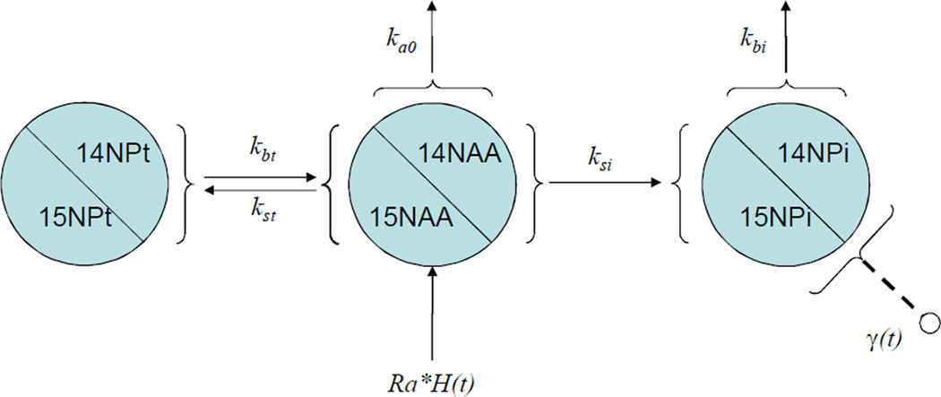
As described in the Results section, the two-compartment model fit the peptide/protein incorporation relative fraction curves well for proteins in mouse brain. However, the two-compartment model fit poorly to proteins in the liver. An examination of the relative fraction incorporation curves from liver protein revealed that the curves cannot be fitted well even with the general two-exponential functions (see Results section for detailed discussion). Therefore, we added an additional total protein compartment to construct a three-compartment model, shown in Figure 3.
Figure 3.
Three-compartment model for protein turnover in liver. The compartments are the free amino acid pool (14NAA/15NAA), the total protein pool (14NPt/15NPt), the protein-of-interest pool (14NPi/15NPi). VAA, VPt, and VPi are the volumetric sizes of the free amino acid pool, the total protein-bound pool, and the individual protein-bound pool, respectively.
The inclusion of the total protein pool is justified because the amino acid recycling by protein degradation and protein export in liver must be considered. The detailed derivation of the three-pool model functional form is given in the supplemental material. A full three-compartment model accounting for both total protein export and total protein degradation (illustrated in Figure S1 of the supplemental material) requires definition of five rate constants. However, we found the fitting of the five-parameter system was not robust because the optimization procedure can easily be trapped in a local minimum. The value for the rate constants for both the total protein degradation into free amino acid (kbt) and the total protein export (k0t) should be small because they are normalized by the large volumetric size of the total protein pool. Indeed, the five-rate constant values for good fits showed that the total protein export rate constant was typically the smallest one. Thus, we removed the rate constant for total protein export from consideration in order to reduce the degree of parametric dimension, resulting in a four-rate constant system (Figure 3). The relative concentration of 15N-labeled amino acid in each protein of interest is
| (23) |
in which
| (24) |
| (25) |
| (26) |
| (27) |
| (28) |
The solution contains three exponentials. A general form of three-exponential function (y (t) = 1+y1e−k1t + y2e−k2t + y3e−k3t) requires six parameters for its definition. Here only four parameters—kst, total protein synthesis rate constant; kbt, total protein degradation rate constant; k0a, amino acid out flow rate constant; kbi, individual protein degradation rate constant—completely define our three-compartment model. In other words, the system has four degrees of parametric freedom. When the function was used to fit the experimental incorporation curves, the fitness was similar to the fittings with the full five-parameter function containing the total protein export rate constant.
RESULTS
All data are from experiments previously described7. The data processing for the 15N distribution of peptide ions was described6. Fitting the compartment model functional forms using 15N distribution data was done similarly as described6. Briefly, the relative 15N fraction was calculated according to Equation 22 and the peptide incorporation curves were constructed from the relative 15N fraction data points against the incorporation times. The relative 15N fraction incorporation curves of the peptide ions belonging to a protein were aggregated to the protein 15N incorporation curve by use of a similarity selection procedure after the shared peptides were removed. In order to guarantee the quality of the protein incorporation curves, we only considered the curves obtained by aggregation of at least two peptide curves and that contained at least four nonzero data points out of nine incorporation times. Still, there were 705 and 797 protein curves to consider in brain and liver, respectively. The supplemental material contains the protein 15N relative fraction incorporation curves among with the fitted rate constants.
Relative isotope fraction
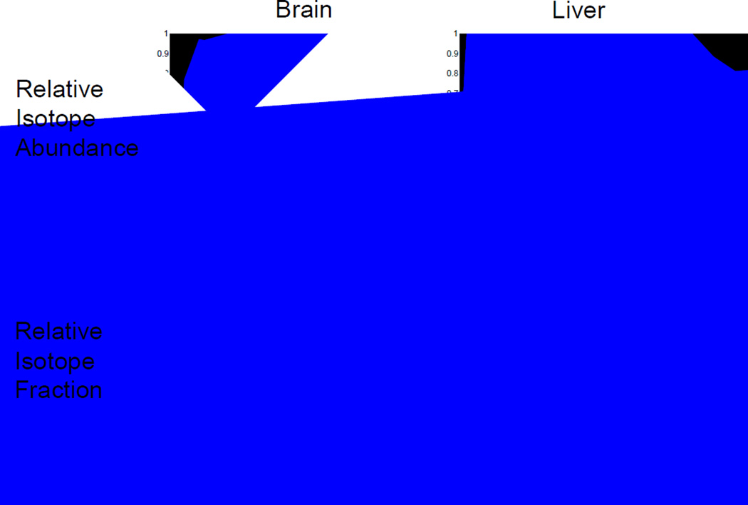
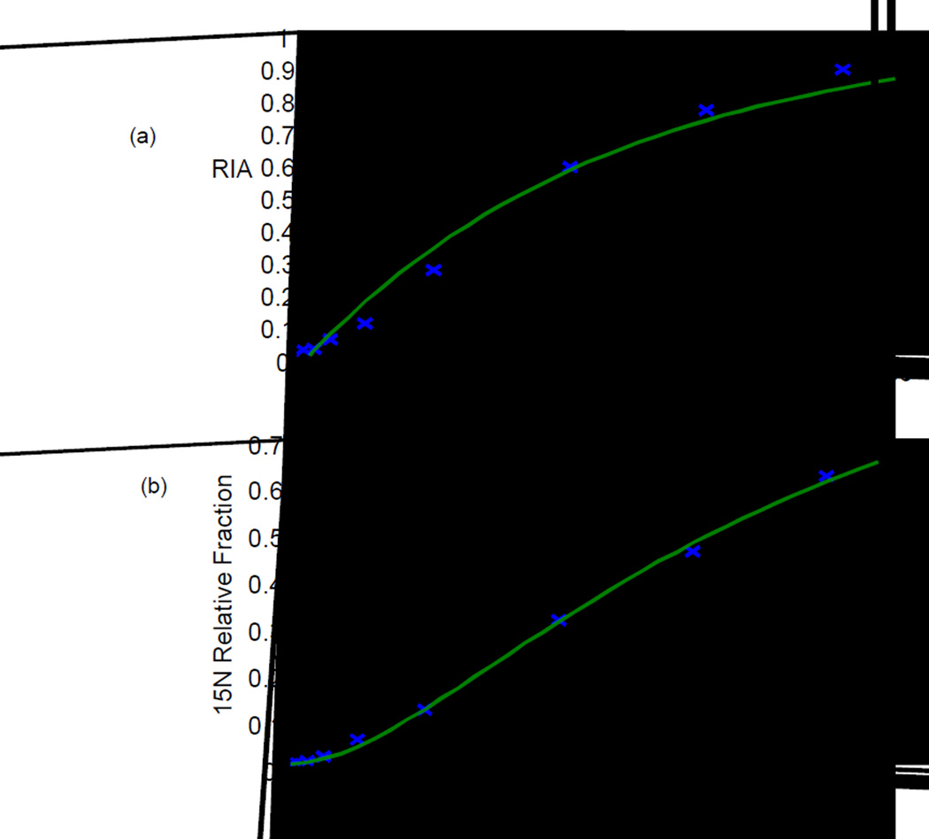
As discussed in the theoretical section, relative 15N fraction (substituting for 15N-labeled amino acid concentration) provides a direct connection of compartment models to the experimental observation. An additional advantage of using relative isotope fraction instead of the commonly used relative isotope abundance (RIA) is illustrated in Figure 4. For proteins with rapid turnover, the incorporation curves using relative isotope abundance (RIA) can quickly reach saturation. This is quite common for many proteins in liver (Figure 4, upper right). In comparison, no proteins attain saturation with the incorporation curves using relative isotope fraction (Figure 4, lower panels).
Figure 4.
Peptide incorporation curves constructed by use of relative isotope abundance (RIA; top panels) or by use of relative isotope fraction, defined by Equation 22 (bottom panels). Peptide curves are from brain proteins (left panels) and from liver proteins (right panels).
Brain proteins: two-compartment modeling
The relative 15N fraction incorporation curves for brain proteins were subjected to a nonlinear regression procedure to fit the theoretical function of Equation 21 for the two-compartment model. Compared to the empirical delayed exponential function (β(t) = 1−e−k0(t−t0), for which k0 is the rate constant and t0 is the time delay) to fit the relative isotope abundance proposed in7, the two-compartment function fit better for almost all of the 700 protein relative fraction incorporation curves from brain although both models use two fitting parameters (Figure 5).
Figure 5.
Fitting protein incorporation curves by used a delayed exponential function for relative isotope abundance (a) and by use of the two-compartment model function of Equation 21 for relative isotope fraction (b).
Shown in Figure 5 are two curve fittings of the same protein (phosphatidylethanolamine-binding protein 1, P70296). The fitting was much more precise for the two-compartment model (Figure 5, lower trace). The rate constant obtained from the two-compartment model (0.0373 day−1) is approximately 40% smaller than that of 0.0563 day−1 from the delayed exponential fit (Figure 5, upper trace).
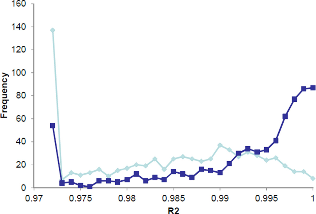
The improvement in fitting of the two-compartment model over the delayed exponential function for all the selected brain proteins is illustrated in Figure 6. The majority (>70%) of the two-compartment model fitting had R2 values of 0.99 or better. In the case of the delayed exponential fit, a smaller portion (<40%) can be fitted equally or better.
Figure 6.
Brain protein incorporation curve fitting. Fitness comparison of the delayed exponential function for relative isotope abundance (gray trace) and the two-compartment model function for relative isotope fraction (black trace).
It is interesting to examine the extreme cases of the functional form of Equation 21. If the protein degradation rate constant, kb, is much smaller than the amino acid removal constant k0, or kb << k0 the solution (Equation 21) reduces to a single exponential function (one compartment).
| (29) |
One additional disadvantage for using the delayed exponential function is the sensitivity of the fit with early incorporation time points. If the delay factor is positive, the delayed exponential function becomes negative when the incorporation time is small. This is, of course, inconsistent with the definition of relative isotope abundance, which should have a possible range from zero to one. One can consider eliminating the early incorporation time points; however, such a choice is subjective and a data processing procedure based on such input is not robust.
Any nonlinear fitting requires an initial parametric value. The fitting of the two-compartment model is robust. For all the protein curves tested, the fitting converged to the global minimum with the same initial values for both rate constants. It is perhaps not surprising here because there are only two degrees of parametric freedom in this system.
Liver proteins: three-compartment modeling
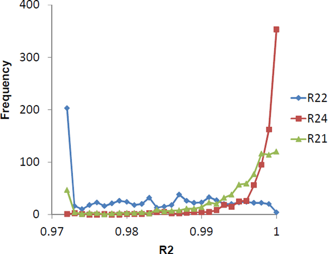
When attempting to fit the 15N relative fraction incorporation curves for liver proteins with the two-compartment model function of Equation 21, a high degree of deviation was observed (Figure 7). In fact, the two-compartment model fitted more poorly than the delayed exponential function, which is equivalent to a general one-exponential function (1-y0e−kt, in which y0 and k are the fitting parameters). Using a general two-exponential function (γ (t) = 1+y1e−k1t + y2e−k2t with four parameters) did not produce better fitting (data not shown). Introduction of the third total protein compartment produced much-improved fitting for most proteins in liver, even when the number of the fitting parameters was kept at four. A typical example is shown in Figure 8, in which the 15N relative fraction incorporation curve for the protein transitional endoplasmic reticulum ATPase (Q01853) was constructed from 37 of its peptide incorporation curves. In a liver protein turnover study with 14C labeling11, a three-exponential function was found to be more appropriate.
Figure 7.
Liver protein incorporation curve fitting. Fitness comparison of the delayed exponential function for relative isotope abundance (gold trace, R21), the two-compartment model function for relative isotope fraction (blue trace, R22), and the three-compartment model function for relative isotope fraction (red trace, R24).
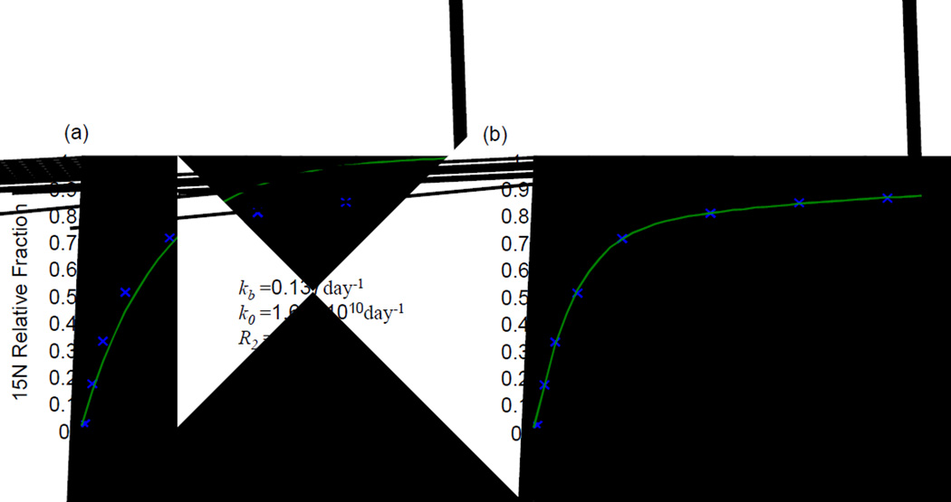
Figure 8.
Illustration of curve fitting for a liver protein, transitional endoplasmic reticulum ATPase. The two-compartment model function fitting with two rate constants (a), and the three-compartment model function fitting with four rate constants (b).
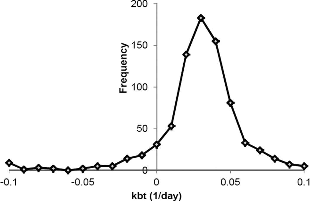
The two-compartment model fitted poorly with the protein degradation rate constant of 0.137 day−1 and the three-compartment model fitted nearly perfectly with the data for the protein degradation rate constant of 0.317 day−1. It is interesting to note that the total protein degradation rate constant (kbt) is very small. This perhaps should not be surprising because the total protein pool size is very large compared to that for free amino acids in a tissue as discussed for the single-compartment model. The statistical analysis of all total protein degradation rate constants for liver proteins support this statement (Figure 9). The median value of the total protein degradation rate constants for all the liver proteins was approximately 0.04 day−1, which is at least one order of magnitude smaller than the other rate constants. Many total protein degradation rate constants had negative values. Of course, these negative values cannot be correct. From an experimental point of view, this can be explained by a situation in which the variation caused by observation errors is larger than the expected values.
Figure 9.
Histogram of total protein degradation rate constants obtained by use of the three-compartment model function for fitting relative 15N fraction incorporation curves of liver proteins.
DISCUSSION
In the theoretical section, we introduced a series of compartment models with increasing sophistication in order to fit the experimentally observed data better. The most important development here is the realization that the relative isotopically labeled fraction can serve as a direct connection between compartment modeling and the experimental data. The relative isotope fraction can be accurately extracted from a single survey scan spectrum from its isotopic peaks without the need to introduce an external factor for its normalization. In a typical dynamic SILAC experiment, if the detected peptide contains a single labeled amino acid, the relative isotope abundance is equal to the relative fraction concentration. However, if the peptide of interest contains more than one labeled amino acid, the relative isotope fraction is a more appropriate indication of the relative amino acid concentration of the peptide instead of the relative isotope abundance.
In a typical large-scale protein turnover study, a large number of high quality protein incorporation curves are available because each can be constructed by use of many (sometimes hundreds) peptide incorporation curves. The compartment models presented here seem able to provide optimal functional forms for fitting the experimental data. For brain proteins, the two-compartment model with only two parameters provided superior fitting compared to any two-parameter functional forms with single compartment models, demonstrating the importance of the correct functional forms. For liver proteins, we attempted to produce a three-compartment model with a minimal number of parameters. A more general three-compartment model with five rate constants, including that for total protein export, is described in the supplemental material. But with the five-parameter system, it was difficult to produce satisfactory fits to the experimental data because it is more sensitive to the initial parameter estimates. The four-parameter system was more robust and produced substantial improvement over the less sophisticated models.
We have also compared the rate constants obtained by fitting relative isotope fraction with compartment modeling against those from fitting relative isotope abundance with the empirical delayed exponential function (see supplemental Figures S1 and S2). In general, the correlations were strong and the ranking order of magnitude was kept in the two data sets. Therefore, the functional analysis given previously7 remains valid. But the values of the rate constants do differ. For brain proteins, the range and values of kbs from the two-compartment model were smaller than those from the delayed exponential fit. This may result from the reduction of outliers in the two-compartment modeling, which separates the contribution of the amino acid removal better than the simple delayed exponential model. This effect was more dramatic for the liver proteins. For the majority of the liver proteins, the individual protein degradation rate constants exhibited a wider range. The delayed exponential modeling seems incapable of accurately extracting individual degradation rate constants with small values for liver proteins. The compartment modeling by use of the relative amino acid concentration (proportional to the relative isotope fraction) has a disadvantage of being unable to separate the compartment size from its rate constant. For example, under the present modeling framework, a small relative isotope fraction can result from either a small portion of completely labeled proteins or all proteins labeled with a small level of labeling. Additional theoretical and informatics development is needed to explain the two extreme cases.
Supplementary Material
ACKNOWLEDGMENTS
This work was supported by NIH NCRR grants RR01614 (to ALB), RR019934 (to ALB), NIH grants AG010770 (to SBP) and AG021601 (to SBP) as well as gifts from the G. Harold and Leila Y. Mathers Charitable Foundation and the Sherman Fairchild Foundation.
ABBREVIATIONS
- RIA
Relative isotope abundance
- SILAC
Stable isotope labeling with amino acids in culture
- SILAM
Stable isotope labeling of mammals
REFERENCES
- 1.Colby DW, Prusiner SB. Nat. Rev. Microbiol. 2011;9:771–777. doi: 10.1038/nrmicro2650. [DOI] [PMC free article] [PubMed] [Google Scholar]
- 2.Claydon AJ, Beynon RJ. Methods Mol Biol. 2011;759:179–195. doi: 10.1007/978-1-61779-173-4_11. [DOI] [PubMed] [Google Scholar]
- 3.Doherty MK, Hammond DE, Clague MJ, Gaskell SJ, Beynon RJ. Journal of proteome research. 2009;8:104–112. doi: 10.1021/pr800641v. [DOI] [PubMed] [Google Scholar]
- 4.Pratt JM, Petty J, Riba-Garcia I, Robertson DH, Gaskell SJ, Oliver SG, Beynon RJ. Mol Cell Proteomics. 2002;1:579–591. doi: 10.1074/mcp.m200046-mcp200. [DOI] [PubMed] [Google Scholar]
- 5.Price JC, Guan S, Burlingame AL, Prusiner SB, Ghaemmaghami S. Proc. Natl. Acad. Sci. USA. 2010;107:14508–14513. doi: 10.1073/pnas.1006551107. [DOI] [PMC free article] [PubMed] [Google Scholar]
- 6.Guan S, Price JC, Prusiner SB, Ghaemmaghami S, Burlingame AL. Molecular & cellular proteomics : MCP. 2011 doi: 10.1074/mcp.M111.010728. [DOI] [PMC free article] [PubMed] [Google Scholar]
- 7.Price JC, Guan S, Burlingame A, Prusiner SB, Ghaemmaghami S. Proceedings of the National Academy of Sciences of the United States of America. 2010;107:14508–14513. doi: 10.1073/pnas.1006551107. [DOI] [PMC free article] [PubMed] [Google Scholar]
- 8.Carson ER, Cobelli C, Finkelstein L. The Mathematical modeling of metabolic and endocrine systems. New York: john Wiley & Sons; 1983. [Google Scholar]
- 9.Wolfe RR, Chinkes DL. Isotope Tracers in metabolic Research. 2nd ed. Hoboken, New Jersey: John Wiley & Sons; 2005. [Google Scholar]
- 10.Senko MW, Beu SC, McLafferty FW. Journal of the American Society for Mass Spectrometry. 1995;6:229–233. doi: 10.1016/1044-0305(95)00017-8. [DOI] [PubMed] [Google Scholar]
- 11.Garlick PJ, Waterlow JC, Swick RW. Biochem J. 1976;156:657–663. doi: 10.1042/bj1560657. [DOI] [PMC free article] [PubMed] [Google Scholar]
Associated Data
This section collects any data citations, data availability statements, or supplementary materials included in this article.


