A synthetic biology approach to the development of transcriptional regulatory models and custom enhancer design

Abstract

Synthetic biology offers novel opportunities for elucidating transcriptional regulatory mechanisms and enhancer logic. Complex cis-regulatory sequences—like the ones driving expression of the Drosophila even-skipped gene—have proven difficult to design from existing knowledge, presumably due to the large number of protein-protein interactions needed to drive the correct expression patterns of genes in multicellular organisms. This work discusses two novel computational methods for the custom design of enhancers that employ a sophisticated, empirically validated transcriptional model, optimization algorithms, and synthetic biology. These synthetic elements have both utilitarian and academic value, including improving existing regulatory models as well as evolutionary questions. The first method involves the use of simulated annealing to explore the sequence space for synthetic enhancers whose expression output fit a given search criterion. The second method uses a novel optimization algorithm to find functionally accessible pathways between two enhancer sequences. These paths describe a set of mutations wherein the predicted expression pattern does not significantly vary at any point along the path. Both methods rely on a predictive mathematical framework that maps the enhancer sequence space to functional output.

1. Introduction

The discovery that a large fraction of the genome, previously classified as “junk DNA”, is responsible for the precise patterning of gene expression, has led to the development of sequenced-based models seeking to predict how and when a gene will express. These efforts have been aided by an ever increasing collection of cis-regulatory elements (commonly called enhancers), revealed through computational, empirical, and comparative approaches. A wealth of data for transcriptional modeling has also become available from initiatives to map the binding of all known transcription factors (TFs) in model organisms [1, 2, 3]. At the biochemical level, steady progress has been made in elucidating mechanisms involved in transcriptional regulation, chromatin dynamics, and transcription initiation and elongation [4, 5, 6]. As our understanding of gene regulation grows so to does the predictive capability of transcriptional models. The methods we describe here now dramatically expand the use of synthetic biology to create artificial enhancers [7, 8].

Eukaryotic regulatory modules are complex, finely tuned molecular machines, with multiple protein-protein, protein-DNA and protein-promoter interactions that are best understood using a quantitative model-based approach [9, 10]. Employing a quantitatively transcriptional model to design novel enhancers offers the opportunity to significantly increase the rate by which our understanding of transcription regulation grows. By using the predictive capability of a transcriptional regulatory model to design DNA sequences with a target expression pattern, these synthetic sequences create empirically testable challenges to the model, i.e. the sufficiency of the model’s regulatory mechanisms. Instances where the observed expression deviates from prediction are of special importance because they provide opportunities to improve upon the model’s regulatory mechanisms. Newly acquired data can be used to refit an improved model in an iterative cycle where new synthetic constructs generated using the new model are synthesized and tested (Fig. 1). Such an approach changes the nature of transcriptional regulatory research by providing a principled, model-based method for investigating regulatory interactions in their native context rather then relying on simpler component-based methods. In non-model based approaches, emergent properties of systems that rely on multiple interactions cannot be formulated as a testable hypothesis.

Figure 1. Iteration cycle for the systematic improvement of a transcriptional model.

The NEEA algorithm and the SA sequence search methodology can be used to increase both the scope and precision of a transcriptional model. The numbers label the separate steps in the cycle and the arrows describe the flow of information between the steps. 1) The cycle starts with a set of known enhancer sequences and their corresponding quantitative expression patterns. 2) Each sequence is scored for the presence of binding sites using PWMs. Open and blacked-filled shapes represent activators (+ effect) and repressors (− effect) respectively. As an illustration, binding site prediction of the 4 main regulators of MSE2 are shown. 3) The known regulatory mechanisms by which TFs influence transcription, along with the predicted TFBSs, binding affinity, and TF concentrations are used to determine the set of all protein-protein and protein-DNA interactions. The diagram shows both competitive binding and quenching interactions for MSE2. Binding sites are colored coded for relative binding affinity. Activators and repressor are shown over and below the line respectively. The quenching efficiency is shown along the horizontal axis by a symmetrical gradient centered on each repressor. Quenching of activator binding sites within the range of a repressor will result in decreased occupancy of the site. 4) The parameters describing the intensity, range, and effect of all interactions are fitted by minimizing the sum of the squared differences between the observed and predicted expression across all constructs and data points. The optimization procedure can produce multiple functional models. 5) SA is used in conjunction with a functional model to search the sequence space for novel enhancers predicted to express in the same pattern to that of an enhancer in the previous iteration. SA can also be used to find enhancers predicted to express in a target expression pattern or that allow discrimination between alternative models. 6) NEEA can be used to find a functionally accessible path between an enhancer in a previous iteration and a novel, functionally equivalent sequence. Sequences sampled at intervals along the path are then synthesized for empirical analysis. 7) Synthesized sequences predicted to express in either conserved or divergent patterns are cloned into an expression vector and their activity assayed in vivo. Shown is a fluorescent in situ hybridization of a Drosophila embryo expressing lacZ driven by the MSE2 enhancer. Confocal images of multiple embryos are analyzed in order to derive the quantitative expression pattern. The new set of enhancers and their corresponding functional output are then added to the previous set for the next round of the iteration.

The application of synthetic biology to the problem of eukaryotic enhancer design has proven to be more challenging then for bacteria where the design and synthesis of cis-regulatory elements has yielded valuable insights [7]. The multimerization of known transcription factor binding sites (TFBSs) [8], for example failed to produce synthetic enhancers that mimic the expression of four Drosophila regulatory elements. While small (100–200 bp) synthetic cis-regulatory elements have been successfully used in the analysis of short-range repression in the Drosophila embryo [11, 12], such elements lack the complexity of wild type enhancers such as the even-skipped (eve) minimum stripe 2 element (MSE2), which contain, to date, thirteen characterized regulatory sites bound by five different transcription factors [13, 14].

The work presented here discusses two methods for generating synthetic regulatory elements. Importantly, these methods are not limited to any particular model nor are they wed to a particular transcriptional regulatory system. The first method uses simulated annealing (SA) to rapidly search the DNA sequence space for novel sequences that express in defined patterns. The second method utilizes a novel search algorithm called NEEA (Neutral Enhancer Evolutionary Algorithm), for finding functionally accessible mutational paths between enhancer sequences, defined as an ordered path for mutations transforming a starting sequence to an ending sequence that does not significantly change the expression pattern at any given point along the path. The SA sequence search answers the question: given available knowledge of a transcriptional system, what are the limits to the type of expression patterns possible? The NEEA algorithm addresses the question: given a known enhancer and expression pattern, at what point along a functionally accessible path does the model prediction break down?

2. Description of methods

Here we illustrate the two methods using a previously described transcriptional model and the well-characterized eve MSE2 enhancer as a test case [15]. The MSE2 enhancer drives transcription in a narrow traverse stripe placed along the anterior-posterior (A P) axis of Drosophila blastoderm embryos between 35% and 45% egg length (EL, 0% at the anterior pole) [13] (Fig. 1, step 7). The activity of the MSE2 is regulated mainly by four TFs: Bicoid (Bcd), Hunchback (Hb), Giant (Gt), and Krüppel (Kr). The domain of expression is set by broad transcriptional activation provided by Bcd and Hb, while Giant and Krüppel set the anterior and posterior boundaries by transcriptional repression respectively [13]. Previously, we had shown that a transcriptional model could successfully predict the effects of mutations in the 1.7 kb upstream eve promoter sequence which contains the MSE2 enhancer [15]. We have built on this work by implementing an automatic TFBS prediction step in the model, thus allowing functional predictions to be made directly from the cis-regulatory sequence. TFBSs were predicted using position weight matrices (PWMs) to calculate the log-odd score of the DNA sequence as in [16]. PWMs for Bcd, Hb, Gt, and Kr were derived from SELEX data obtained from the Berkeley Drosophila Transcription Network Project (BDNTP). Because our previous analysis of the 1.7 kb eve promoter sequence suggested that the TFs Caudal (Cad), Tailless (Tll), and Knirps (Kni) also play a role in refining the eve stripe 2 pattern, the model includes PWMs for these factors (PWMs for Knirps and Tailles were obtained from [17] while SELEX data was used for Cad). Only those sequences with log-odd scores above a previously determined threshold were considered binding sites (Fig. 1, step 2). Threshold values were set such that they recovered all of the previously footprinted binding sites for each TF.

Our modeling approach is based on the assumption that transcription is an enzymatic reaction wherein the RNA Pol II holoenzyme must overcome an energy barrier for transcription to initiate. The binding of an activator to its binding site is postulated to reduce the energy barrier by an amount proportional to the fractional occupancy of the site. In contrast, transcriptional repressors are postulated to quench nearby activator binding sites by reducing their fractional occupancy. Previous work in this system has shown that the quenching efficiency starts to decrease linearly at distances of 50 bp from the repressor, with no measurable quenching effect at distances over 150 bp [12]. A detailed description of the mathematical framework describing the transcriptional model is given in the Supplementary Information (S1).

A crucial requirement of both methods is the existence of a previously fitted transcriptional model that can be used to give an initial prediction of enhancer output. To this end, division cycle 14A (C14A) embryos carrying a P-element eve-lacZ reporter driven by the MSE2 enhancer (line 1511B, gift from M. Levine) were collected, fixed and stained for eve-lacZ mRNA by in situ hybridization as in [15]. Embryos were then classified as belonging to time classes 2 to 6 (T2–T6) of C14A as in [18]. Quantitative eve-lacZ expression profiles along the A–P axis for each time class were obtained as previously described [15] and used as a reference pattern for the initial model fit. The model parameters describing the regulatory interactions were determined by minimizing the summed squared difference between the model output and the observed data. TF concentration profiles of Bcd, Hb, Gt, Kr, Cad, Kni, and Tll along the A–P axis of C14A embryos were obtained from the FlyEx database (http://flyex.uchicago). Because the concentration of ligand factors important for the transcriptional regulation at the terminal pole regions of the embryos have not been determined, model fits and calculations are carried out only from 35% to 92% EL along the embryo A–P axis. Optimization was performed using the Lam simulated annealing schedule [19, 20, 21]. The C source code for the model, SA sequence search, and the NEEA algorithm can be downloaded from http://flyex.uchicago.edu/newlab/download.shtml.

2.1. Simulated annealing sequence search

The problem of finding novel enhancer sequences with a desired functional output represents an enormously difficult task. The difficulty lies both in the large size of the search space, as well as in the complexity of the cost function, defined here as the sum of the squared differences between the target gene expression and the model prediction across the set of all observed data points and their associated TF concentrations. For example, the size of the search space for finding a 480 bp sequence that is functionally equivalent to the MSE2 enhancer is of approximately 10²⁸⁸ sequences! Likewise, the large number of possible protein-DNA and protein-protein interactions result in a highly nonlinear cost function with a complex landscape of peaks and valleys that make optimization difficult. The complexity of the cis-regulatory logic of wild type enhancers is readily apparent in a diagrammatic representation of all quenching and DNA-protein interactions in the MSE2 enhancer (Fig. 1, step 3). In order to solve this problem, a previously described method of simulated annealing [19, 20] was adapted to efficiently search the sequence space for enhancers that minimize the cost function.

2.1.1. Overview of simulated annealing (SA)

The SA optimization method is a global optimization method that can be used without any restrictions on the search space. It is based on making an analogy between the real physical annealing processes and the problem of optimization in a high dimensional search space [22]. In metallurgy, annealing involves heating a metal to a starting temperature T₀ such that it glows red hot. As the metal reaches T₀, the bonds between the atoms of the metal break allowing them to randomly diffuse until they reach an equilibrium energy configuration determined by the Boltzmann distribution of the ensemble at T₀. If the temperature is then cooled very slowly, the system maintains a quasi-equilibrium such that at any given temperature T, the system remains in a Boltzmann distribution. As the temperature decreases to 0, the energy configuration of the ensemble converges to the global minimum. Analogously, SA introduces an artificial temperature parameter T, which determines the probability of accepting or rejecting moves along the search space according to the Metropolis criterion [23]. In SA, the last evaluation of the cost function E is regarded as the “energy” of the system while the current parameter values x⃗ correspond to the state or “energy configuration”. Starting from an initial random state $\overrightarrow{x_0}$ and a starting temperature T₀, the algorithm samples the search space in an iterative cycle consisting of:

1. from current state $\overrightarrow{x_n}$ propose a move to state $\overrightarrow{x_p}$

2. calculate the energy increment $\mathrm{\Delta }E=E(\overrightarrow{x_p})-E(\overrightarrow{x_n})$

3. accept the move to state $\overrightarrow{x_p}$ with probability p(ΔE) = min(1, exp(−ΔE/T))

4. repeat until the system is frozen

After each iteration, the temperature is decreased according to a specific cooling schedule. The system is considered frozen when it has reached a pre-determined temperature, or when no more moves can be accepted at the current temperature. If the temperature is cooled slowly, the iterative sampling of the search space according to the Metropolis criteria results in a time-averaged energy of the system that approaches that of an ensemble of states distributed according to the Boltzmann distribution. Thus like in the physical system, as T goes to 0, the energy configuration of the system approaches that of the global minimum.

2.1.2. Implementation

In what follows, we describe the specifics of the SA sequence search method, and show through in silico experiments that it can efficiently search the sequence space.

Let n be the total number of data points (i.e. the total number of conditions, spatial, or temporal coordinates) for which we are evaluating the cost function, and let m be the total number of different TFs in the model. We define $\overrightarrow{v_j}$ as the vector composed of the input TF concentrations {v₁(j),…, v_m(j)} associated with the data point j. Without loss of generality, we can then write the cost function as

$$E(S_i)=\sum _{j=1}^n{(\mathcal{T}(j)-\mathcal{M}(S_i,\overrightarrow{v_j}))}^2,$$ (1)

where E(S_i) is the value of the cost function for the candidate sequence S_i, (j) is the target gene expression at data point j, (S_i, $\overrightarrow{v_j}$) is the model output given sequence S_i and the vector of input TF concentrations $\overrightarrow{v_j}$ at data point j.

In the case where we are using the previously fitted transcriptional model in order to find 480 bp sequences that are functionally equivalent to the MSE2 enhancer, the cost function E(S_i) (Eq. 1) is summed over 290 data points consisting of 58 nuclei (35% to 92% EL) and 5 time classes (T2–T6). Each of the 290 data points is associated with a set of measured concentration values for Bcd, Hb, Gt, Kr, Cad, Kni, and Tll.

The SA sequence search is an implementation of the Lam adaptive SA method [19, 20]. An important characteristic of adaptive SA is that it draws upon the statistical record the SA process in order to dynamically determine the rate of temperature decrease and the average proposed move size. In the case of SA sequence search, we define a move as a set of k random point substitution that takes the system state from sequence S_n to sequence S_n+1 and where k corresponds to the move size. The process is initiated with a random sequence S₀ of length l. During each iteration, we select a move size k from an exponential distribution with a mean of Θ. A proposed move of k random point substitutions is made, and the new sequence S_n+1 is accepted or rejected according to the Metropolis criterion as previously described. Statistics on the number of accepted and rejected moves are collected for 100 iterations, after which the algorithm adjusts the size of Θ such that the acceptance ratio (moves accepted/total number of moves) is maintained at approximately 0.44; a value chosen on the basis of previous theoretical analysis [19, 20]. In addition, statistics that allow for the estimation of the energy variance are collected and used in conjunction with the acceptance ratio in order to determine the size of the temperature decrease.

Previous work had suggested that the efficiency of the parameter search, is maximized when the variance of the distribution of energies of proposed moves is as large as possible. Moreover, it has been claimed that this occurs when the acceptance ratio is maintained at 0.44 [19, 20]. However, this result had not been previously verified in our system. We decided to check the validity of this claim to test whether the SA sequence search method was searching the sequence space with maximum efficiency. In addition, we also decided to check whether our move size controller was capable of maintaining the proper acceptance ratio. Statistical data on the move size, acceptance ratio, and the variance of the ΔE of proposed moves was collected at four different temperatures during an SA sequence search for 480 bp sequences that are functionally equivalent to MSE2. Plotting the acceptance ratio as a function of move size shows that the acceptance ratio decreases monotonically with increasing move size (Fig. 2), indicating that it is possible to adaptively regulate the acceptance ratio by increasing or decreasing the average number of mutations per move. Likewise, a scatter plot of the variance of the ΔE of proposed moves with respect to the acceptance ratio, shows that the maximum variance occurs at 0.44 (Fig. 3). This result is in perfect agreement with the result previously derived by Lam [19, 20].

Figure 2. Increasing the average move size results in a decrease in the acceptance ratio of proposed moves.

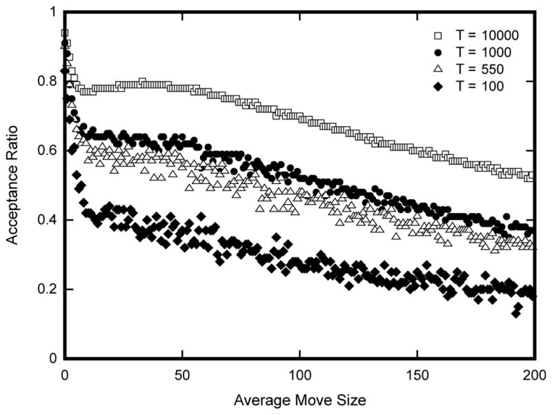
Each point in the graph corresponds to the average acceptance ratio of 10⁵ proposed moves. Acceptance ratio was calculated as the number of accepted moves over the total number of proposed moves from a fixed point in the annealing run. Average move size corresponds to the average number of substitutions per annealing step. Data were collected at four different temperatures during the annealing process (10⁴, 10³, 550, and 100). Simulated annealing was carried out with an initial temperature of 10⁶ and allowed to cool according to the Lam adaptive schedule. Once the annealer reached the specified equilibrating temperature, the temperature was kept constant and statistics on acceptance ratios were recorded. Average move size at each equilibrating temperature was increased from zero to two hundred in increments of one.

Figure 3. The maximum standard deviation of the delta energies of proposed moves occurs at 0.44 acceptance ratio.

Data were collected under the same conditions as in Fig. 2, where each point represents the standard deviation of the ΔE of 10⁵ proposed moves. ΔE’s were calculated as the energy differentials between the current states and those of the proposed moves. The dashed lines corresponds to an acceptance ratio of 0.44 and occurs at approximately the maximum standard deviation at all four temperatures.

2.2. Neutral Evolutionary Enhancer Algorithm (NEEA)

A well established principle in evolution is that all transitional states between two adaptive phenotypes must themselves be adaptive. Borrowing from this evolutionary principle, we imagine that between any two functionally equivalent sequences (i.e. with a conserved expression pattern) S and S′, there exists a minimum ordered set of single point mutations transforming sequence S to S′ along a functionally accessible path. We define a functional accessible path as one wherein for any given sequence S_i along the path, E(S_i) (Eq. 1) is below a user-defined viability threshold t, and where the target gene expression corresponds to the conserved reference pattern. The sequences could be for example, homologous sequences from two related species or the sequence from an extant species and from an ancestral node inferred from a phylogeny. Alternatively, we might ask the question of whether it is possible to find a functionally accessible path that connects a wildtype enhancer with a functionally equivalent synthetic sequence, or between two synthetic enhancers with a conserved functional output. In this section we describe the NEEA algorithm, its requirements, and the different optimization methods it uses during each step.

2.2.1. Sequence alignment

The NEEA algorithm requires an alignment between a starting and ending sequence. The alignment can be produced in several ways; we use the Wagner-Fischer algorithm for minimizing the Levenshtein or minimum edit distance between two sequences [24]. The Levenshtein distance is defined as the minimum number of edits (single nucleotide substitutions, insertions, and deletions) linking the starting and ending sequences. The minimum edit distance provides a measure of the degree of separation of two sequences, and is a commonly used metric in maximum parsimony methods that seek to reconstruct phylogenetic trees [24]. Once an alignment has been established, the algorithm determines the initial minimal set of mutations as differences between the two sequences. Consecutive deletions can be treated either as a single mutational event or as independent point deletions. Each point substitution, insertion, or deletion is considered a single mutation.

Since the sequence alignment determines the set of inferred mutations between sequences, the code is able to exhaustively evaluate alternative Wagner-Fischer alignments and trace different evolutionary trajectories for each. However, since the number of alignments tends to grows factorially with the edit distance, it is only possible to evaluate all of them exhaustively when the edit distance is small. For those cases where there is a large edit distance between the two sequences, one approach might be to use a constrained alignment algorithms such as the Morphalign software, that uses PWMs and phylogenetic information for improved alignments of homologous enhancer sequences [25].

2.2.2. Optimization of mutation order

Using the mutational set derived from the alignment, the next step is to order the set to find an functional accessible path linking the sequences. Let {S₁, …, S_n} be the set all n sequence in a path. We define the path cost function P as

$$P=max\{E(S_1),\dots ,E(S_n)\},$$ (2)

where P is the path cost function, and E(S_i) is the model cost function (Eq. 1 evaluated at sequence S_i of the path. Eq. 2 seeks to minimize the maximum value of E along the path. In order to speed up the code, each possible intermediate sequence is kept in memory along with the calculated cost function.

Minimization of the path cost P is achieved by using two separate optimization procedures. The first optimization uses an adaptation of a dynamic hill descent algorithm which quickly finds regions of local minima [26]. The procedure involves applying a transformation to the permutations so that the optimization can occur in a vector space; once a move occurs in the vector space a reverse transformation is applied to calculate P [27]. The transformation function is defined as

$$b_{a_j}=\sum _{i=1}^{i=j}\{\begin{array}{ll}1\hfill & \text{if}{a}_i>a_j\hfill \\ 0\hfill & \text{if}{a}_i<=a_j\hfill \end{array}$$ (3)

where {a₁, a₂, …, a_n} is a permutation of n integers from the ordered set {1, 2, …, n}, and {b₁, b₂, …, b_n} is the resulting vector, with 0 <= b_j <= n − j.

This function (Eq. 3) transforms the permutation space into a vector space of dimension n-1, where n is the number of elements to permute. A search for local minima is carried out by evaluating different possible directions in the vector space to find path cost decreases. Once a direction is selected, the search vector magnitude is doubled in order to more rapidly find the local minima. If a direction that decreases P is not found, the search vector is decreased in magnitude by half. The search ends when the magnitude of the search vector drops below a threshold such that the current best permutation order cannot be improved upon. By starting out at multiple random positions in the vector space, different local minima can be found. The local minimum with the lowest path cost is then chosen for further optimization. Algorithm 1 in the Supplementary Information (S1) shows the pseudocode describing the dynamic hill climbing method.

The second optimization step is carried out in its entirety in the permutation space. After finding a local minimum, the mutations along the path are indexed in descending order of their calculated E. The optimization procedure involves testing out all the possible n-1 swaps of the highest scoring mutation until P is reduced. If no swaps are found to reduce P, the next highest scoring mutation is swapped. This algorithm is repeated until P is reduced or all possible pairwise permutations are tested. Once a swap has reduced the score, the mutations are re-indexed in descending score value and the swapping starts again from the highest scoring mutation. The procedure ends when no further path cost reducing swaps are found. Alternatively, the algorithm can also be stopped after the index of the mutation to be swapped exceeds a previously defined threshold. This can be useful in cases where the total number of pair-wise swaps becomes too large to compute. By starting from a region close to a local optimum, the second optimization procedure allows for a deeper exploration of the search space in this region to obtain better results.

2.2.3. Path fragmentation

After the optimization of the path cost function is complete, the maximum score value of the evolutionary trajectory is compared to the viability threshold. A maximum score lower then the viability threshold indicates that it has found a viable evolutionary trajectory. If the maximum score is higher, the algorithm will seek to find a new trajectory by breaking up the path into smaller segments. This is achieved by searching for an intermediate sequence in the immediate vicinity of the maximum scoring sequence that has a score lower than the viability threshold. A new path optimization procedure is then carried out between the starting point and the intermediate sequence, as well as between the intermediate sequence and the ending point. The search for an intermediate sequence employs simulated annealing to find the lowest scoring sequence within a small edit distance radius of the maximum scoring sequence. In order to carry out the search, random point mutations are applied to the maximum scoring sequence and the new sequence score value is calculated (Eq. 1). If the resulting sequence has a higher score then the viability threshold, the search is restarted with a larger search space. The search space is increased by enlarging the edit distance radius by small increments. The procedure is repeated until a new sequence is found that falls within the viability threshold. In this way, a viable scoring sequence is found which adds the smallest possible number of additional mutations to the mutation set and trajectory.

Once an intermediate point is found, a new alignment is determined between the starting point and the intermediate sequence as well as the ending point sequence. A new evolutionary trajectory is then calculated by applying the optimization procedure outlined above on both segments separately. If there are still points outside the viability threshold, the path fragmentation procedure is applied recursively until a viable path is found. The intermediate points along the path represent can be thought of as representing “hidden” states that are not observable when comparing the starting and ending points alone. Parallel and convergent evolution are two well known mechanisms that create hidden states in DNA sequences.

2.3. Application

One challenge in modeling is to distinguish among competing models that “explain” the data. The use of artificially designed enhancers can be a powerful tool to achieve this aim. By using simulated annealing to design enhancers, it is possible to find sequences that are predicted to express differently under competing models. These sequences can then be synthesized and tested in vivo. In other words, rather than using the algorithm to find a sequence that minimizes Eq. 1, it is possible to find a sequence such that given model A and model B, the sequence maximizes the cost function

$$E(S_i)=\sum _{j=1}^n\left({\mathcal{M}}^A(S_i,\overrightarrow{v_j})-{\mathcal{M}}^B(S_i,\overrightarrow{v_j})\right),$$ (4)

where (S_i, $\overrightarrow{v_j}$) and (S_i, $\overrightarrow{v_j}$) are the predicted expression pattern of sequence S_i at data point j of models A and B respectively, and $\overrightarrow{v_j}$ is the set of TF concentrations at data point j.

Maximizing Eq. 4 typically results in a sequence S where the expression pattern predicted by model A over-expresses with respect to that predicted by model B. By switching the positions of (S_i, $\overrightarrow{v_j}$) and (S_i, $\overrightarrow{v_j}$) in Eq. 4, it is possible to select which model over-expresses. As an example, Fig. 4A shows the result of using simulated annealing to search for sequences that differentiate between two models both of which correctly predict eve stripe 2 expression. Importantly, the search for sequences that maximize Eq. 4 provides a systematic way to determine the true value of model parameters where the two models differ. The rational design of test sequences by this approach is expected to pinpoint short-comings in models and should lead to more rapid improvement in models of enhancer structure/function.

Figure 4. Applications of simulated annealing on sequence.

(A) Method for distinguishing between two alternative models of transcriptional regulation. Simulated annealing was used to find a DNA sequence that maximizes the differences between model predictions. Dashed line corresponds to sequence A/B that is predicted to express strongly throughout most of the embryo by model A, but would have no expression under model B. Solid line represents sequence B/A predicted to express in an anterior-posterior gradient under model B, but is predicted not to express under model A. Top and bottom panels show predictions by model A and B respectively. (B) Method for generating arbitrary expression patterns. Simulated annealing was used to design enhancers predicted to express in target expression patterns. Top panel shows a collection of predicted 480 bp synthetic enhancers that would drive expression in a stripe pattern at different A–P positions along the embryo. Bottom panel shows a 4 kb synthetic enhancer predicted to express in an arbitrary target pattern. Model prediction is in red while target expression pattern is in black. Horizontal axis for panels A and B show A–P embryo position in percent egg length length. Vertical axis for panels A and B shows relative mRNA concentration. Dashed line in panel B depicts the no-expression reference point for mRNA expression. (C) Method for creating an ensemble of functionally equivalent enhancers. Simulated annealing was used to generate a collection of 10⁵ 480 bp enhancer sequences predicted to express in a D. mel eve stripe 2 expression pattern. Each dot represents a synthetic enhancer sequence. Sequences were generated by sampling the annealing process every 10⁵ moves at three different equilibrating temperatures. Red, blue, and green dots represent sequences sampled at annealing temperatures of 100, 10, and 1 respectively. Horizontal axis shows the minimum edit distance between the synthetic sequence and the D. mel MSE2. Vertical axis shows the calculated root mean squared difference between the model prediction and the observed D. mel MSE2 pattern used as reference. Figure inserts show predicted expression patterns of representative sequences sampled at different temperatures. Red line corresponds to model prediction while dashed line corresponds to the reference MSE2 expression pattern.

Another important application of simulated annealing on sequence is the ability to create arbitrary expression patterns. Once a model has been developed that shows a good predictive ability, it is possible to use simulated annealing to generate custom-made synthetic enhancers within the natural limits of the system. Because TFs can act combinatorially to produce a vast array of expression patterns, it is possible possible to create sequences that drive a wide array of different patterns of gene expression. This capacity can be of use in both basic research as well as in applied settings. In research, synthetic enhancers predicted to express in novel patterns can be a powerful tool for model validation. It is also possible to use custom-made enhancers in experiments that require the expression of a particular gene in a pattern that does not currently exist in nature. Alternatively, synthetic enhancers can be used in biomedical applications such as tissue or genetic engineering. A major limitation in gene therapy is the small DNA carrying capacity of many viral vectors (5–8 kb) used to transfer therapeutic genes to the patient [28]. Thus, the ability to create a minimal length synthetic enhancer capable of driving expression in the proper cells could provide a significant advancement in this area. Fig. 4B shows the use of simulated annealing, in conjunction with a model of eve stripe 2, to create artificial enhancers expressing in arbitrary patterns. It is important to note however, that the ability to create novel patterns is limited by the nature and expression profiles of the interacting transcription factors acting on the system. Thus, as more transcriptional regulatory systems fall under study, a wider range of expression patterns will be possible.

A recurring question in transcriptional regulation is, what are the design principles guiding the construction of enhancers? SA sequence search is expected to shed light on this problem as well. During the annealing process, as the temperature parameter is progressively lowered, the solution to the optimization problem gets closer and closer to the global minimum. By stopping the annealing process at a particular temperature and allowing the optimization algorithm to equilibrate (i.e. maintaining the temperature constant while continuing to make moves according to the Metropolis criterion), it is possible to generate an ensemble of an arbitrary large number of synthetic constructs that fit a particular pattern by sampling the annealer at periodic intervals. The creation of a large ensemble allows for the discovery of common design elements among multiple enhancers. In addition, novel insights regarding robustness can be gleaned by a comparative analysis among the different synthetic enhancers as well as between the synthetic enhancers and wild type constructs. Fig. 4C shows an ensemble of approximately 10⁵ non-homologous synthetic enhancers predicted to express in an eve stripe 2 pattern.

The NEEA algorithm allows for the discovery of functionally accessible paths between cis-regulatory elements. A direct application of this method is the use of NEEA to determine the most likely order of the mutational events along the branches of a phylogenetic tree. Under the assumption of a strong functional constraint, the root mean squared (rms) difference between the reference and predicted expression pattern can be used as a proxy for the fitness conferred by a given sequence. Given the current lack of information on how subtle changes in expression patterns translate to changes in fitness, the algorithm does not try to calculate a fitness value from the rms score. Rather, the algorithm seeks to find an evolutionary pathway where the predicted rms score at each point is below a given rms threshold. This threshold value, called the viability threshold, can be determined a priori by selecting the maximum predicted rms value observed among extant homologous sequences assumed to have evolved under a functional constraint. An example of functionally accessible evolutionary paths between closely related species can be seen in Fig. 5A.

Figure 5. Applications of the Neutral Enhancer Evolutionary Algorithm (NEEA).

(A) Method for finding functionally accessible evolutionary paths between ancestral and extant enhancer sequences. The ancestral mel-sim-sec eve stripe 2 enhancer sequence was predicted using Bayesian inference. Functionally accessible evolutionary paths between the ancestral stripe 2 sequence and the corresponding sequence in sim, sec, and mel were generated using the NEEA algorithm. Dashed line corresponds to the viability threshold wherein sequences with a calculated cost function above the line are non-viable. Paths were generated such that at all points the calculated cost function E were below the viability threshold. In addition, a penalty of 0.01 was used in Eq. 2 in order to minimize the variance of E along the path. Vertical axis shows the value of E at that each point along the path. Horizontal axis depicts the number of mutations separating the D. mel stripe 2 enhancer from the current point along the path. (B) Method for creating a collection of functionally equivalent enhancers with decreasing homology. First, simulated annealing was used to generate a synthetic DNA sequence expressing in a D. mel MSE2 pattern. To maximize the probability of generating a functional enhancer, the sum of the squared differences between the predicted and the reference pattern of seven separate models were added together. A functionally accessible path was generated between the wild type mel MSE2 sequence and the synthetic enhancer using the NEEA algorithm. In this case the objective was to give greater weight to the shape of the pattern then to the amplitude. For this purpose both the predicted and observed expression patterns were normalized on a scale of 0 to 1. Cost functions were calculated as the sum of the squared differences between the normalized patterns. To prevent under-expression, the value of E was multiplied by the fold under-expression between the reference and observed patterns prior to normalization. Fold under-expression was calculated as the ratio between the maxima of the reference and predicted patterns. As in the case of simulated annealing, the cost function evaluations of seven separate models were added together to provide a new cost function used in the NEEA optimization algorithm. The vertical axis shows the total added score of seven models while the horizontal depicts the number of mutations separating the wild type MSE2 from the synthetic sequence. A total added score of 12 was used as the viability threshold in the optimization.

The final application discussed here is the use of the NEEA algorithm as a tool for determining the limits of model predictability. The methodology involves first using simulated annealing to create a synthetic enhancer predicted to express in a similar pattern to a given wild type sequence. The second step is to use NEEA to trace a functionally accessible pathway from the wild type to the synthetic enhancer. The functionally accessible path provides a set of sequences, all predicted to give approximately the same expression pattern, but which become progressively diverged from the starting wild type enhancer sequence. Sequences along the path can then be sampled along regular intervals, synthesized and their expression measured, to determine if there is a point along the path where the model predictions break down. The sequence at which the predictions deviate from the observations can be compared to the sequence at a previous step in order to isolate the key mutational changes responsible for the loss of predictability. This approach can then be used systematically to improve the accuracy of the model and has the potential to yield insight into novel regulatory mechanisms and transcription factors involved in the regulation of the system under study. Using NEEA a functionally accessible mutational path was traced between the eve MSE2 and a synthetic sequence of the same length also predicted to express in a stripe 2 pattern (Fig. 5B).

Data-driven modeling approaches, which are becoming the norm in studies of regulatory elements, place a premium on tools that can take advantage of systems biology techniques. The work presented here is a step in this direction, providing a systematic and clear methodology for the validation and improvement of current regulatory models. The use of de novo synthesized elements in combination with optimization algorithms, maximizes the information content of data-driven approaches by rapidly localizing the current limits of model predictability. Through multiple iterative cycles of predictions, synthesis, evaluation, and fitting, it is possible to create models with progressively greater predictive power (Fig. 1). These models can in turn be of great importance in tissue engineering or experimental applications where expression patterns not currently available in nature might be required.

References

- 1.Celniker SE, Dillon LA, Gerstein MB, Gunsalus KC, Henikoff S, Karpen GH, Kellis M, Lai EC, Lieb JD, MacAlpine DM, Micklem G, Piano F, Snyder M, White KP, Waterston RHT modENCODE Consortium. Nature. 2009;459:927–930. doi: 10.1038/459927a. [DOI] [PMC free article] [PubMed] [Google Scholar]
- 2.NN, et al. Nature. 2011;471:527–531. [Google Scholar]
- 3.modENCODE Consortium. Science. 2010;330:1787–1797. doi: 10.1126/science.1198374. [DOI] [PMC free article] [PubMed] [Google Scholar]
- 4.Nechaev S, Adelman K. Biochimica et Biophysica Acta. 2011;1809:34–45. doi: 10.1016/j.bbagrm.2010.11.001. [DOI] [PMC free article] [PubMed] [Google Scholar]
- 5.Suganuma T, Workman JL. Annual Review of Biochemestry. 2011;80:473–499. doi: 10.1146/annurev-biochem-061809-175347. [DOI] [PubMed] [Google Scholar]
- 6.Selth LA, Sigurdsson S, Svejstrup JQ. Annual Review of Biochemistry. 2010;79:271–293. doi: 10.1146/annurev.biochem.78.062807.091425. [DOI] [PubMed] [Google Scholar]
- 7.Amit R, Garcia HG, Phillips R, Fraser SE. Cell. 2011;146:105–118. doi: 10.1016/j.cell.2011.06.024. [DOI] [PMC free article] [PubMed] [Google Scholar]
- 8.Johnson LA, Zhao Y, Golden K, Barolo S. Tissue Engineering Part A. 2008;14:1549–1559. doi: 10.1089/ten.tea.2008.0074. [DOI] [PMC free article] [PubMed] [Google Scholar]
- 9.Reinitz J, Hou S, Sharp DH. ComPlexUs. 2003;1:54–64. [Google Scholar]
- 10.Arnosti DN. Annual Review of Entomology. 2003;48:579–602. doi: 10.1146/annurev.ento.48.091801.112749. [DOI] [PubMed] [Google Scholar]
- 11.Fakhouri WD, Ay A, Sayal R, Dresch J, Dayringer E, Arnosti DN. Molecular Systems Biology. 2010;6:341. doi: 10.1038/msb.2009.97. [DOI] [PMC free article] [PubMed] [Google Scholar]
- 12.Hewitt GF, Strunk B, Margulies C, Priputin T, Wang XD, Amey R, Pabst B, Kosman D, Reinitz J, Arnosti DN. Development. 1999;126:1201–1210. doi: 10.1242/dev.126.6.1201. [DOI] [PubMed] [Google Scholar]
- 13.Small S, Blair A, Levine M. The EMBO Journal. 1992;11:4047–4057. doi: 10.1002/j.1460-2075.1992.tb05498.x. [DOI] [PMC free article] [PubMed] [Google Scholar]
- 14.Andrioli LPM, Vasisht V, Theodosopoulou E, Oberstein A, Small S. Development. 2002;129:4931–4940. doi: 10.1242/dev.129.21.4931. [DOI] [PubMed] [Google Scholar]
- 15.Janssens H, Hou S, Jaeger J, Kim AR, Myasnikova E, Sharp D, Reinitz J. Nature Genetics. 2006;38:1159–1165. doi: 10.1038/ng1886. [DOI] [PubMed] [Google Scholar]
- 16.Hertz GZ, Stormo GD. Bioinformatics. 1999;15:563–577. doi: 10.1093/bioinformatics/15.7.563. [DOI] [PubMed] [Google Scholar]
- 17.Rajewsky N, Vergassola M, Gaul U, Siggia ED. BMC Bioinformatics. 2002;3:30. doi: 10.1186/1471-2105-3-30. [DOI] [PMC free article] [PubMed] [Google Scholar]
- 18.Surkova S, Kosman D, Kozlov K, Manu, Myasnikova E, Samsonova A, Spirov A, Vanario-Alonso CE, Samsonova M, Reinitz J. Developmental Biology. 2008;313:844–862. doi: 10.1016/j.ydbio.2007.10.037. [DOI] [PMC free article] [PubMed] [Google Scholar]
- 19.Lam J, Delosme J-M. Technical Report 8816. Yale Electrical Engineering Department; New Haven, CT: 1988. An efficient simulated annealing schedule: Derivation. [Google Scholar]
- 20.Lam J, Delosme J-M. Technical Report 8817. Yale Electrical Engineering Department; New Haven, CT: 1988. An efficient simulated annealing schedule: Implementation and evaluation. [Google Scholar]
- 21.Reinitz J, Sharp DH. Mechanisms of Development. 1995;49:133–158. doi: 10.1016/0925-4773(94)00310-j. [DOI] [PubMed] [Google Scholar]
- 22.Kirkpatrick S, Gelatt CD, Vecchi MP. Science. 1983;220:671–680. doi: 10.1126/science.220.4598.671. [DOI] [PubMed] [Google Scholar]
- 23.Metropolis N, Rosenbluth A, Rosenbluth MN, Teller A, Teller E. The Journal of Chemical Physics. 1953;21:1087–1092. [Google Scholar]
- 24.Gusfield D. Algorithms on strings, trees, and sequences. Cambridge University Press; 1997. [Google Scholar]
- 25.Sinha S, He X. PLoS Computational Biology. 2007;3:e216. doi: 10.1371/journal.pcbi.0030216. [DOI] [PMC free article] [PubMed] [Google Scholar]
- 26.Yuret D. PhD thesis. Massachusetts Institute of Technology; 1994. From Genetic Algorithms to Efficient Optimization. [Google Scholar]
- 27.Turrini S. Technical Report. Western Research Laboratory; 1996. Optimization in Permutation Spaces. [Google Scholar]
- 28.Kay MA, Glorioso JC, Naldini L. Nature Medicine. 2001;7:33–40. doi: 10.1038/83324. [DOI] [PubMed] [Google Scholar]