GPU linear and non-linear Poisson–Boltzmann solver module for DelPhi

Abstract

Summary: In this work, we present a CUDA-based GPU implementation of a Poisson–Boltzmann equation solver, in both the linear and non-linear versions, using double precision. A finite difference scheme is adopted and made suitable for the GPU architecture. The resulting code was interfaced with the electrostatics software for biomolecules DelPhi, which is widely used in the computational biology community. The algorithm has been implemented using CUDA and tested over a few representative cases of biological interest. Details of the implementation and performance test results are illustrated. A speedup of ∼10 times was achieved both in the linear and non-linear cases.

Availability and implementation: The module is open-source and available at http://www.electrostaticszone.eu/index.php/downloads.

Contact: walter.rocchia@iit.it

Supplementary information: Supplementary data are available at Bioinformatics online

1 INTRODUCTION

The Poisson–Boltzmann equation (PBE) is a widely used tool to estimate the electrostatic energy of molecular systems in ionic solution. Given the continuously increasing size of structural data for proteins and other macromolecules and the need to deal with bigger and more complex structures, the availability of tested and reliable algorithms on the most recent and affordable computational architectures, such as Graphical Processing Units (GPUs), is highly desirable. In this context, we present an implementation on a GPU architecture of both a linear and a non-linear PBE solvers based on the finite difference (FD) scheme. The first use of an FD approach to solve the PBE can be ascribed to Warwicker and Watson (1982). Our implementation follows that adopted by the DelPhi solver and described in Nicholls and Honig (1991), which exploits the checkerboard structure of the FD discretization of the Laplace differential operator and adopts successive over relaxation to converge to the solution. To our knowledge, this is the first description of a GPU implementation of the non-linear PBE, which follows the same approach used by DelPhi and detailed in Rocchia et al. (2001). Our implementation can be executed on any NVIDIA card with Compute Unified Device Architecture (CUDA) capabilities.

2 SERIAL NUMERICAL SOLUTION

The PBE rules the electrostatic potential of a system where free charges and dipoles react to fixed charges located on the solute. This can be thought of as an extension of the Debye–Huckel continuum electrostatic theory [see Debye and Huckel (1923)]. It is successfully used in biophysics to estimate the electrostatic energy of biomolecular systems in ionic solution as shown by Grochowski and Trylska (2007). From the mathematical standpoint, the PBE is a second order, elliptical and non-linear partial differential equation, which, in the case of a monovalent salt dissolved in the solution, takes the following form:

(1)

where is the electrostatic potential, ϵ is the local relative dielectric constant, is the permittivity of the vacuum and is null inside the solute and it equals the reciprocal of the Debye length in the solution. This equation can be rewritten in a way that isolates the non-linear dependence on the potential:

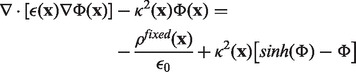(2)

This form is particularly suitable for devising the non-linear algorithm as an adaptation of the linear one, according to a perturbative approach. The FD discretization of the PBE and application of the successive over-relaxation method leads to the following iteration stencil:

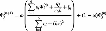(3)

where q_j is the discretized fixed charge, h is the grid spacing, ξ accounts for the non-linear correction, if present, and ω is the over-relaxation factor. The best value for ω can be obtained, in the linear case, from the highest eigenvalue of the iteration matrix as seen in Stoer and Bulirsch (2002). This method is stable, as the iteration matrix is diagonally dominant. In the non-linear case, over-relaxation can lead to divergence and an adaptive method to assign ω is used, as detailed in Rocchia et al. (2001). Dirichlet boundary conditions are usually adopted based on the analytical solution of the linearized PBE in spherical symmetry, a few considerations on possible alternatives can be found in Rocchia (2005).

3 GPU IMPLEMENTATION

The GPU implementation borrows from the algorithm originally given by Nicholls and Honig (1991). All the calculations related to the stencil are done on the GPU card (or equivalent device). Interestingly, the stencil in Equation (3) shows a checkerboard (‘odd and even’) structure, implying that updating a point requires only the knowledge about its nearest neighbors, which are of opposite parity. Therefore, the execution can be divided in two segments, alternating the update of odd and even points. Within each segment, the calculations are independent, so any further parallelization is trivial. Therefore, the physical grid is partitioned in two logical subgrids, odd and even. Our GPU implementation further exploits this structure and loads alternately odd and even points to the ‘texture’ memory of the device to optimize the memory access. Dedicated data structures separately address charged grid points, and those that are at the boundary between regions with different dielectric. A thread starts from every grid point of the bottom xy slice of each subgrid and then proceeds along the z direction. A single step along z in a subgrid corresponds to an increment of two in the physical grid. Nearby threads in a xy slice of a subgrid are gathered in blocks and are given access to a common shared memory. Basically, a thread does a loading step, followed by an updating step and finally it moves to the upper slice in the same subgrid. For example, before updating an odd point a thread loads to the shared memory the even point having its same index. Because all the threads of a block act in parallel, and thanks to a purposely designed indexing scheme, an odd thread block in one step loads simultaneously all the even grid points needed for the updating task with the exception of the neighboring points that pertain to the adjacent blocks and of those that are in the z direction. We cope with the first problem by adding a suitable overlap between blocks borders. The ‘z − 1’ and the ‘z + 1’ points of the physical grid are not present in the shared memory and therefore need further accesses to the ‘texture’ memory. The number of these accesses is halved by saving each ‘z + 1’ point in a temporary variable, which plays the role of the ‘z − 1’ point once the thread has moved to the upper slice. In the Supplementary Material, a graphical description of the algorithm is provided, whereas a more detailed explanation in the case of the linear PBE is given in Colmenares et al. (2013). Similarly to the DelPhi approach, the non-linearity is treated as an additive charge-like term, which affects only the grid points that are located in solution and which is gradually inserted during the solution. Whether to update the non-linear term is decided at the CPU level, based on a heuristic approach as in the DelPhi code [Rocchia et al. (2001)].

4 RESULTS

The results in Table 1 show the speedup between the serial code executed on a CPU with an AMD Opteron (1.4 GHz) chip and a Tesla Kepler K20m. The solver was run on the fatty acid amide hydrolase protein with 8325 atoms. A monovalent salt concentration of 0.15 M was used. The relative dielectric constant of the molecule was taken as 2.0 and that of the solution as 80.0. The Debye length is roughly 8 Å. The speedup of the non-linear algorithm is comparable with that of the linear one. In fact, the former benefits from a larger number of floating point operations but it suffers from a larger number of data transfers.

Table 1.

Fatty acid amide hydrolase protein—8325 atoms—297 × 297 ×297 grid points

Computing step	Linear solver	Non-linear solver
	GPU (CPU, speedup)	GPU (CPU, speedup)
Boltzmann	9.060 s (1 min 31 s, ×10.05)	8.83 s (1 min 28 s, ×9.96)
Iteration	0.015 s (0.18 s, ×10.60)	0.035 s (0.44 s, ×12.57)
Total	10.250 s (1 min 38 s, ×9.61)	10.14 s (1 min 37 s, ×9.55)

Note: The execution time is reported per computing step: ‘Boltzmann’ includes the overall time spent for Laplace and Boltzmann updates. ‘Iteration’ is the time spent in a single iterative step. ‘Total’ includes all the iterations and the initialization of the GPU card.

REFERENCES

- Colmenares J, et al. 21st Euromicro International Conference on Parallel, Distributed and Network-Based Processing (PDP) 2013. Solving the linearized Poisson-Boltzmann equation on GPUs using CUDA; pp. 420–426. [Google Scholar]
- Debye P, Huckel E. Zur theorie der elektrolyte. Physik. Zeits. 1923;24:185–206. [Google Scholar]
- Grochowski P, Trylska J. Continuum molecular electrostatics, salt effects, and counterion binding - Review of the Poisson-Boltzmann theory and its modifications. Biopolymers. 2007;89:93–113. doi: 10.1002/bip.20877. [DOI] [PubMed] [Google Scholar]
- Nicholls A, Honig B. A rapid finite difference algorithm, utilizing successive over-relaxation to solve the Poisson-Boltzmann equation. J. Comput. Chem. 1991;12:435–445. [Google Scholar]
- Rocchia W. Poisson-Boltzmann equation boundary conditions for biological applications. Math. Comput. Modell. 2005;41:1109–1118. [Google Scholar]
- Rocchia W, et al. Extending the applicability of the nonlinear poisson-boltzmann equation: multiple dielectric constants and multivalent ions. J. Phys. Chem. B. 2001;105:6507–6514. [Google Scholar]
- Stoer J, Bulirsch R. Numerical Mathematics. Berlin Heidelberg New York: Springer; 2002. [Google Scholar]
- Warwicker J, Watson H. Calculation of the electric potential in the active site cleft due to -helix dipoles. J. Mol. Biol. 1982;157:671–679. doi: 10.1016/0022-2836(82)90505-8. [DOI] [PubMed] [Google Scholar]
Associated Data
This section collects any data citations, data availability statements, or supplementary materials included in this article.