Closing yield gaps: perils and possibilities for biodiversity conservation

Abstract

Increasing agricultural productivity to ‘close yield gaps’ creates both perils and possibilities for biodiversity conservation. Yield increases often have negative impacts on species within farmland, but at the same time could potentially make it more feasible to minimize further cropland expansion into natural habitats. We combine global data on yield gaps, projected future production of maize, rice and wheat, the distributions of birds and their estimated sensitivity to changes in crop yields to map where it might be most beneficial for bird conservation to close yield gaps as part of a land-sparing strategy, and where doing so might be most damaging. Closing yield gaps to attainable levels to meet projected demand in 2050 could potentially help spare an area equivalent to that of the Indian subcontinent. Increasing yields this much on existing farmland would inevitably reduce its biodiversity, and therefore we advocate efforts both to constrain further increases in global food demand, and to identify the least harmful ways of increasing yields. The land-sparing potential of closing yield gaps will not be realized without specific mechanisms to link yield increases to habitat protection (and restoration), and therefore we suggest that conservationists, farmers, crop scientists and policy-makers collaborate to explore promising mechanisms.

1. Introduction

Demand for food is rising and options to expand the area devoted to producing it are diminishing [1,2]. Agricultural yields are well below attainable levels in many parts of the world, and so ‘closing yield gaps’ is widely viewed as an important part of securing a sufficient and reliable food supply [3,4]. However, past initiatives to increase yields have caused serious negative impacts on wild species living on farmland [5,6]. Closing yield gaps using fertilizers and irrigation could exacerbate such impacts. At the same time, agricultural expansion poses a great threat to wild habitats and species [1,7]. This threat could potentially be reduced if closing yield gaps can be successfully linked to initiatives to spare land for nature [8,9]. In this paper, we use an illustrative global analysis to look at how conservationists and agronomists might decide where closing yield gaps would be most harmful to biodiversity, and where doing so might be most beneficial.

(a). Why focus on yield gaps?

Some argue that a focus on yields distracts from more important issues such as reducing food waste, distributing food more fairly and shifting towards diets which are less land-demanding [10–13]. However, even if good progress is made with these important challenges, global food demand will increase substantially over the next few decades [14]. This increased demand will be met by some combination of increasing the area under agriculture and increasing yields on existing land. In recognition that both of these processes tend to have negative impacts on wild species, there have been recent efforts to begin to quantify trade-offs between biodiversity value and yield [15–23]. Understanding such trade-offs can help conservationists to decide where and to what extent they should support land-sharing strategies (which aim to integrate food production and biodiversity conservation on the same land, but which frequently incur the penalty of lowered yields) as opposed to land-sparing strategies (which aim to spare land for nature by producing food from as small an area of land as possible) [8,24,25].

Before pursuing a land-sparing strategy in a particular region, it is important to understand whether the impacts on on-farm biodiversity of increasing yields are potentially outweighed by the benefits of using higher yields to minimize the area occupied by farmland. Recent work in southwest Ghana and northern India suggests that they would be, for a range of bird and tree species in those landscapes [15]. More work is needed to understand when and where land sparing, land sharing or a mixed approach is most appropriate for a range of outcomes, not just for food production and biodiversity, and also the most effective ways of delivering these strategies in practice [26]. We argue here that understanding the spatial distribution and magnitude of yield gaps in relation to the distribution of species with different types of response to agriculture will be important for identifying areas where the closing of yield gaps presents an opportunity to use land sparing to enhance biodiversity conservation, and others where land sharing could be more appropriate.

(b). Potential risks to biodiversity

The main risks to biodiversity of closing yield gaps are threefold. First, there is the risk that yield-enhancing changes to agriculture will damage populations of species within the farmed landscape [27]. Second, some changes in agricultural practice affect species in non-farmed habitats, for example, through increased nitrogen pollution of rivers and seas [14]. Third, there is the risk that closing yield gaps will increase, rather than decrease, cropland expansion and habitat loss [28].

The detrimental effects of agricultural intensification, both on and off farmland, are widely recognized. Fertilizer use tends to reduce plant diversity, and run-off of nitrates and phosphates causes eutrophication and dead zones in aquatic systems [29]. Irrigation reduces the amount of water available to natural rivers and wetlands, and dams built to supply irrigation water can have serious impacts, especially on migratory species [30]. Pesticides are designed to kill certain wild species, but also typically affect many non-target organisms, including amphibians [31] and pollinators [32]. Shorter rotations and faster growing crops leave less time for crop-dwelling organisms to complete their life cycles or access resources in the intervals before planting or harvesting [33]. Mechanized harvesting can cause direct mortality of birds, insects and other organisms [34]. Use of fossil fuels, fertilizers and manures generates greenhouse gas emissions that affect biodiversity through climate change and ocean acidification [35].

Increasing yields has the potential to promote rather than inhibit local conversion of natural habitats, at least if it is unaccompanied by restrictions on agricultural expansion [36–38]. New crop varieties—such as soya beans that tolerate acidic soils or oil palms that grow well in deep peat—might enhance yields, but at the same time make it feasible to open up new biodiversity-rich areas for cultivation where it is currently not economical to grow these crops [7]. Where higher yields produce higher profits, there may similarly be an increased incentive to expand cropland area [39]. Increased revenues resulting from the closure of yield gaps for staple crops could be used to subsidize expansion of the cultivation of luxury crops and biofuels, again promoting rather than inhibiting the conversion of natural habitats. Therefore, for the potential land-sparing benefits of closing yield gaps to be realized, specific measures to minimize or avoid the conversion of natural habitats to arable production are required [24,37].

(c). Potential opportunities for conservation

Although closing yield gaps poses risks to biodiversity, untapped agricultural potential also presents the opportunity of harnessing yield increases to spare land for nature. While some wild species thrive in agricultural landscapes [40], many depend instead on relatively intact natural habitats, and cannot persist even in ‘benign’ production landscapes [41]. This is particularly true of species of conservation concern, such as those with small global distributions [42–44]. Harnessing yield increases to spare land for nature could also reduce the impacts of farming on biodiversity in other ways, for example, if it reduces greenhouse gas emissions [9,14].

As discussed in §1b, increasing yields will not automatically ensure that land not needed for crop production is spared for nature. Instead, increasing yields only presents the opportunity to spare land for nature, and practical approaches for doing this have not yet been explored in depth [26]. The key requirement for land sparing to succeed is that an explicit connection is made between increasing yields and protecting natural habitats. If the current emphasis in agricultural policy and advocacy circles on closing yield gaps is to be turned into a conservation opportunity, mechanisms need to be developed to integrate yield increases into strategies to spare land for nature.

(d). Aims of this paper

Our aim in this paper is not to provide a definitive assessment of where land sparing or land sharing would be most appropriate for biodiversity conservation. Instead, we aim to provide a conceptual basis for identifying where and by how much closing yield gaps could affect biodiversity, both negatively and positively. We do this with an illustrative analysis combining preliminary estimates of variation in sensitivity of the world's birds to farming with recent work on mapping yield gaps for wheat, rice and maize. We use this approach to suggest where closing yield gaps might pose the greatest risks for bird conservation on cropland, and where cropland expansion—through failure to close yield gaps or indeed as an unintended consequence of successfully doing so—might pose the greatest risks to birds dependent on natural habitats. We focus on birds because they are the only taxon for which the required data are available for a large number of species, and on cereal crops because their great importance in human food supplies has led to yield gaps in these crops being well-studied. These three crops together account for one-third of global cropland area.

2. Material and methods

(a). Crop yields and production

Global maps of attainable yields for wheat, rice and maize were provided by Mueller. Attainable yields are defined in Mueller et al. [4] and are those achievable under local climatic conditions with feasible changes in agricultural practice to address suboptimal availability of water and nutrients. Global maps of estimated ‘current’ (2000) yields and harvested areas for these three crops, obtained using methods described in [45], were provided by Ramankutty (http://www.geog.mcgill.ca/~nramankutty/Datasets/Datasets.html). Projections of the expected quantity of the three crops produced in each country of the world in 2050, as described by Alexandratos & Bruinsma [46], were provided by Alexandratos. These projections were based upon expert judgement of expected demand (including the use of cereals for animal feed and biofuels), international trade flows and the potential for production. In some cases, these estimates were only available for groups of countries rather than individual countries (e.g. the 27 European Union countries, Eastern Europe and some of the smaller developing countries, including many of the island nations: we assumed in such cases the same percentage increase for each country as for the group). We used a global map of cropland [47] to develop country-level estimates of cropland area and non-cropland area. Missing production and area data were extracted from the FAO [48]. All maps consisted of 5-min grid cells (≈10 × 10 km).

We considered 171 countries in our analysis: all of the countries are listed by Mueller et al. [4], plus 16 not included there. Of these 171 countries, 14 small island nations had no overlap with at least one of the global agricultural datasets we used, and thus we could only produce meaningful results for the remaining 157. Countries are listed in the electronic supplementary material.

(b). Land-sparing potential: definition and estimation of the ‘area at stake’

As a measure of land-sparing potential, we estimated the ‘area at stake’ in each country and grid cell: the difference between the area of cropland needed to meet the projected level of crop production in 2050 with and without the achievement of technically attainable yield increases (figure 1). The ‘area at stake’ is the land which could potentially be spared if yield gaps are closed, and which is at risk of being converted to cropland if they are not. It also includes current cropland which could be taken out of production and restored as natural habitat if yield increases were used to reduce cropland area.

Figure 1.

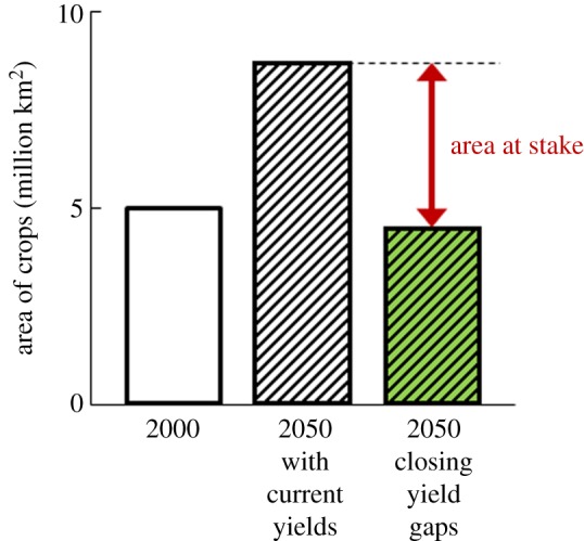
Illustration of the potential effect of closing yield gaps on the future area of land needed for growing maize, rice and wheat. The ‘current’ (2000) global area of these crops is shown by the white bar. The areas required to meet 2050 production projections are shown by the hatched bars for two extreme cases: if yields remained at their ‘current’ (2000) levels (white hatched bar), and if yields were increased to attainable levels (shaded hatched bar). The ‘area at stake’ is the difference between the area needed to meet 2050 production projections if yields remained at their current levels, and the area needed if yield gaps were closed. This land-sparing potential will not be realized without specific policies and incentives to constrain and reverse agricultural expansion. (Online version in colour.)

For each country, we obtained estimates of the production that would be possible for each of the three crops, by summation across all cells within the country currently growing the crops, assuming that attainable yields were completely achieved [4]. We then calculated the cropland area required to produce the projected level of production in 2050 for a country at the attainable yield, derived from Mueller et al. [4]. This area is shown by the shaded hatched bar in figure 1. In doing this calculation, we assumed that any additional cropland needed would be distributed within the country in proportion to the area of land other than cropland present in 2000 in each cell and that the attainable yield for currently uncropped land converted to cropland would equal the mean attainable yield for that country. This assumption was made because the area at stake should include land vulnerable to indirect land-use change prompted by the displacement of other crops, and so will extend beyond areas of high suitability for the three focal crops. Any cropland no longer needed was distributed in proportion to the area of cropland present in 2000 in each cell. This allowed us to calculate the area of cropland that would be required in each cell in 2050, which was summed across the cells within a country. We then repeated these calculations but assumed that yields remained at 2000 levels (white hatched bar in figure 1). The difference between the two estimates of the cropland required in 2050 is the estimated area at stake.

(c). Projected increases in production from closing yield gaps

We estimated the increased production of each of the three crops per grid cell that would be obtained by closing yield gaps enough to match projected production in 2050 in those countries where projected production was less than or equal to attainable production without increasing crop area. In countries where projected production exceeded that attainable on the current cropland area growing these crops, we quantified the production increase up to that given by the attainable yield on the current area. We converted production of each crop, in tonnes, into a common currency, food energy (TJ), using standard conversion factors [49]. We then calculated the total additional food energy from each cell that would be generated through increasing yields to meet the projected production in 2050, or to the attainable yield on the current area growing these crops (if this level of production was smaller). This increase in production was divided by the area of all land in the cell, and expressed as TJ km⁻² yr⁻¹. Our intention in calculating this projected change in production per unit area was to assess the potential risk posed to wild species inhabiting farmland, as large yield increases over extensive areas are likely to be detrimental to most such species [5]. It might be thought that it would have been better to do this simply by calculating the increase in food energy produced per unit area of land used to grow the three crops, rather than the increase in production divided by the area of all land in the cell. We adopted the latter procedure to avoid assigning a large risk to wild species from increasing yield in cells where only a small proportion of the total land area is used to grow these crops, and divided by the area of the cell because cells differ in area with latitude.

(d). Bird range maps

We obtained range maps for all of the world's birds from BirdLife International [50]. These maps show the range in both the breeding and non-breeding seasons, but we used only the breeding range (including areas in which species were resident year-round). We excluded families of birds which are entirely or mainly marine (Alcidae, Chionidae, Diomedeidae, Fregatidae, Gaviidae, Hydrobatidae, Pelecanoididae, Phaethontidae, Procellariidae, Spheniscidae, Stercorariidae and Sulidae). We retained all species in partly marine families where most species in the family also use terrestrial and freshwater habitats (Anatidae, Laridae, Phalacrocoracidae, Podicipedidae and Scolopacidae). We excluded parts of species' ranges where they have been extirpated, as well as areas where they are not native. We also excluded 19 small island endemic species whose ranges did not overlap cells identified as land in our agricultural datasets. This left 9679 species. We conducted our analysis at the resolution of 5-min grid cells (≈10×10 km). A species was considered to be present in a grid cell if any part of its breeding range overlapped the cell.

(e). Predicting species’ responses to changes in yield

We wished to estimate the expected proportion of bird species in a given cell that fell into each of four categories which describe the relationship of their population density to the yield of farming. Such relationships can be used to predict species’ potential population sizes under different production scenarios. We used response types defined in Phalan et al. [15] which used measurements of bird population density and food energy yield averaged over whole farming landscapes and unfarmed areas with natural or semi-natural vegetation in southwest Ghana and northern India. Response types were defined as follows, in relation to the total agricultural production for the region under consideration in the year the data were collected. Loser species are those whose total population in the region, on farmed and unfarmed land combined, is reduced by farming at some levels of agricultural yield and winner species are those for which this is not the case. These two categories were further divided. (i) Losers with the highest total potential population size if farming is at the highest attainable yield, provided that this is combined with protection of natural habitat on all of the land not required for food production. Following earlier studies [8,15], this is defined as a land-sparing strategy, so we call these species SP losers (figure 2a). (ii) Losers with the highest total potential population size with farming at the lowest permissible yield, which would require the use of all available land for food production, leaving none for natural habitats. This is defined as a land-sharing strategy, so we call these species SH losers (figure 2b). (iii) Losers with the highest total populations under a strategy with yield intermediate between the minimum permissible and the maximum attainable are called intermediate (INT) losers (figure 2c). (iv) All winner species were combined into a single category, regardless of the effect of farm yield on their potential total population size (figure 2d–f). Winner species are unlikely to be of unfavourable conservation status because their total populations are larger at all yields than those thought to have prevailed before agriculture was introduced into the region.

Figure 2.

Schematic of different categories of relationships between the population density of individual species and agricultural yields (after [8,15]). The vertical line on each plot represents (for illustrative purposes) the minimum yield that can deliver an agricultural production target. A chord (dashed line) is drawn from the intercept to the point on the density-yield curve corresponding to the yield at which the total population of that species on farmed and unfarmed land combined will be greatest. Its intersection with the vertical line (square) gives relative population size scaled such that the intercept density represents population size in the absence of agriculture. Loser species are those with populations negatively affected by agriculture at some or all levels of yield. (a) SP losers would have their highest overall population when land is farmed at the highest permissible yield and other land is conserved (land sparing). (b) SH losers would have their highest overall population with the lowest permissible yield (land sharing). (c) INT losers would have their highest overall population at an intermediate yield and with an intermediate amount of land spared. (d–f) Winner species are those with population sizes always higher with agriculture than they would be in the absence of agriculture. (Online version in colour.)

The identification of the response type to which a given species belongs by the methods used by Phalan et al. [15] requires detailed data on bird population density and agricultural yield, but these data are only available for a small number of areas [51]. To predict how all terrestrial bird species might respond to changes in farming we used habitat categories and other data from BirdLife International [52] to predict response types. These data form part of the assessments that BirdLife International undertakes for the International Union for Conservation of Nature (IUCN) Red List, and draw on data from a wide range of literature sources and the input of thousands of experts. The importance of each habitat type (following the IUCN Red List classification at http://www.iucnredlist.org/technical-documents/classification-schemes/habitats-classification-scheme-ver3) is coded for each species as being major, suitable or marginal. We assigned a score of 2 for major, 1 for suitable and 0 for marginal/unused habitats. We examined the data for each species for two groups of habitats: (i) those defined in the classification as not being ‘artificial’, which we took to be natural and (ii) those artificial habitats which we considered to be characteristic of arable farmland, that is, ‘arable land’, ‘canals, drainage ditches, ditches’, ‘irrigated land’, ‘ponds (less than 8 ha)’, ‘seasonally flooded agricultural lands’ and ‘water storage areas (more than 8 ha)’. From each of these two groups, we took the highest suitability score of all the habitats assessed within the group. We refer to these maximum scores as Natmax for natural habitats and Artmax for artificial habitats. We then took the difference in maximum suitability score for natural and artificial habitats (Natmax minus Artmax) as a variable likely to be a correlate of response type.

We also used the habitat data to generate covariates representing which natural habitats were of major importance for each species. We scored each of the five broad habitat types of forest, grassland, savannah, shrubland and wetland as 1 if it was coded as of major importance for the species and zero if it was not. We did not consider the broad habitat types of desert, marine coastal/supratidal, marine intertidal and rocky areas (e.g. inland cliffs, mountain peaks), because they were listed as of major importance for too few (five or fewer) of the species from Ghana and India for which we had measured the response type. For each of the five natural habitats included in our analysis, there were at least 15 species in our dataset from Ghana and India for which that habitat was of major importance. We also used as covariates of response type whether the species was migratory or not (scored as zero if the species was listed as ‘not a migrant’ in [52] and 1 if listed as ‘migratory’, ‘altitudinal migrant’ or ‘nomadic’) and the areal extent of the global breeding/resident range of the species: Extent of Occurrence (EOO in millions of square kilometres) [52]. Hence we used eight covariates of response type in all: Natmax–Artmax, EOO, migratory status and the importance of five natural habitats.

We modelled the effect of these covariates on response type using three sets of logistic regression models. First, we assigned each of the 336 species in the dataset for Ghana and India (Ghana 163 species, India 173 species: these totals differ slightly from those in Phalan et al. [15], because we excluded taxa not identified to species level) as a loser species (=1, see above) or a winner (=0) and used this as the binary dependent variable. We fitted logistic regression models using all possible combinations of the eight independent variables, giving a total of 256 models in all, including the null model with no effects but excluding all models with interaction terms. We then calculated the weighted mean of the intercept and the regression coefficient for each of the variables across all models using corrected Akaike information criterion (AIC_c) weights [53]. We also calculated the relative importance of each variable as the sum of the AIC_c weights of all the regression models which included that variable. We then repeated this modelling procedure, except that we included in the analysis only the 220 loser species and assigned each loser species in the dataset for Ghana and India (Ghana 122 species, India 98 species) as a species favoured by land sparing with high-yield farming (SP loser; =1, see above) or another loser type (=0) and used this as the binary dependent variable. Finally, we repeated the procedure with species favoured by low-yield farming (SH losers) being assigned the score 1 in the binary dependent variable and all other loser species being assigned the score zero. For validation purposes, we also performed these three sets of analyses using only the data for Ghana and only the data for India.

(f). Validating regression models of species’ responses to changes in yield

We used the Burnham-Anderson [53] model-averaged regression model parameters and the values of the eight covariates to calculate the expected probability that a given species in the Ghana–India dataset was a loser species and also the probability that the species was an SP loser or SH loser, conditional upon it being a loser. We also calculated the products of the expected probabilities that the species was a loser and the conditional probability that it was an SP or SH loser to give the unconditional probability that a species was an SP or SH loser. We then calculated the area under the curve (AUC) of the receiver operating characteristic (ROC) plot of sensitivity against one minus specificity [54] as a measure of the performance of the regression model in predicting the response type of a species. In order to make this a validation test, we used the model-averaged regressions fitted to only the data for Ghana to predict response types for Indian bird species and vice versa. We also summed the expected probabilities across species for each of the response types, SP loser (unconditional), SH loser (unconditional) and winner, to give the expected proportions of these three response types. The expected proportion of INT losers was obtained as one minus the sum of these three expected proportions.

(g). Mapping importance for species of different response types

For our illustrative analysis, we used the model-averaged logistic regression model based upon the combined results from India and Ghana and eight covariates from BirdLife International [52] to predict the probability that each of the world's terrestrial bird species was a loser species. The probability that it is a winner species is one minus this value. We calculated the importance of each grid cell for winners and losers, using information from BirdLife International [50] on which species breed in the cell. Importance was calculated for each species in each cell as

where a is the land area of the cell in square kilometres, p is the expected probability of the focal species being in a specified response type, calculated from the regression model, and g was the global range size of the species in square kilometres. Values for all species occurring in a cell were summed to produce estimates of its importance for winners and for losers. Global range size was taken into account in this calculation so as to give a higher importance to cells which contained a large proportion of the global range of a species (following [55]).

We used the same procedure to calculate the importance of each grid cell for (i) SP losers and (ii) SH losers. In this case, the expected probability calculated from the regression models for each species was, for SP losers (SH losers), the product of the expected probability of being a loser species and the probability of being an SP species (SH species), conditional on being a loser.

(h). Mapping risks and opportunities

We intersected the map of area at stake (land-sparing potential) with the map of importance for SP losers to identify areas with (i) both a large area at stake and high importance for bird species whose total population size would be greatest with land sparing, and (ii) a large area at stake but low importance for bird species which would do best under land sparing. These areas represent regions where cropland expansion to grow staple crops is likely unless yield gaps are closed, but with different effects of achieving land sparing on the conservation status of birds because of spatial variation in importance for SP loser species.

We produced an equivalent map for SH losers by intersecting the map of projected increases in production from closing yield gaps with the map of importance for SH losers. This identified areas with (i) large projected increases in production if yield gaps are closed and high SH loser importance, i.e. where yield increases are possible and, if realized, could have a large impact on the conservation status of SH loser birds which benefit from low-yielding farming methods, and (ii) large projected increases and low importance, i.e. where yield increases are possible but which are relatively unimportant for SH losers.

3. Results

(a). Crop yields and production

According to the estimates of Alexandratos & Bruinsma [46], global production of wheat, rice and maize is projected to increase by 47%, 38% and 99%, respectively, above 2000 levels by 2050. For maize and rice, projected increases in production by 2050 exceed those achievable on current land devoted to those crops, even if yield gaps are closed by fully achieving attainable yields. For wheat, it would be technically possible at a global level to meet projected 2050 production without further expansion of wheat cultivation if yield gaps are closed.

For all three crops combined, it would be technically possible for around half of the 157 countries analysed to meet projected 2050 production by closing yield gaps on land already devoted to those crops. In most of the remaining countries, projected 2050 production could be met by closing yield gaps together with the modest increases in cropland area. In only five countries would expansion of these three crops require more than 10% of the countries’ non-cropland area even if attainable yields were fully achieved: Bangladesh, Cambodia, El Salvador, The Philippines and Sierra Leone (see electronic supplementary material). Without increases in yield (and/or reductions in projected production) almost all countries would require some cropland expansion: onto more than 10% of their non-cropland in the cases of 31 countries (see electronic supplementary material).

(b). Land-sparing potential: area at stake

Comparing the extent of cropland expansion with and without the achievement of attainable yields identifies places where closing yield gaps has the greatest potential to be used as part of a strategy to spare land for biodiversity conservation in natural habitats, including parts of West and East Africa, southeastern Europe and South and southeast Asia (figure 3a). These are areas where either cropland expansion is most likely if yields are not increased or cropland retraction is most feasible if yields are increased in the countries identified. The total area at stake for the three crops was estimated at 4.2 million km², equivalent to 28% of current global cropland area.

Figure 3.

(a) Area at stake (land-sparing potential) for wheat, rice and maize combined. The scale shows the difference in the additional area of cropland needed to meet projected 2050 production if yields remain at 2000 levels or increase as necessary within attainable levels. Area is calculated in square kilometres per 5-min grid cell, and then divided by the total area of each cell. (b) Projected increase in production between 2000 and 2050, if yield gaps are closed sufficiently (within the constraints of what is attainable) to meet projected production of wheat, rice and maize. Estimates are provided in TJ/year, and divided by the total area of each cell, as cells differ in size with latitude. Map (a) shows area at stake on both cropland and non-cropland, whereas map (b) shows changes only in cells which already have cropland. This and other maps use the Eckert IV projection.

There were eight countries with an area of more than 100 000 km² at stake: India, China, Russia, Brazil, USA, Nigeria, Pakistan and Kazakhstan (‘total area at stake’ in electronic supplementary material). These countries account for half of all cropland and 43% of the global area at stake, and thus changes in agricultural yields and areas in them will have a particularly large influence on global trends.

(c). Projected increases in production from closing yield gaps

By combining information on attainable yields and projected production, we identified the areas with the largest projected increases in production if yield gaps were to be closed. Such areas include in particular parts of south and east Asia (figure 3b). These are the cropland areas in which changes in cereal farming methods are likely to be most dramatic and extensive, and thus where they have most potential to affect populations of wild species living within farmed landscapes.

(d). Correlates of species’ response types

Model-averaged logistic regression modelling of pooled data of response types of bird species in Ghana and India indicated that three variables had a strong influence (relative importance > 0.9) on the probability of a species being a loser (table 1). These were the extent of the global breeding range (negative effect), the importance of grassland as a natural habitat (negative) and the difference in the maximum scores for natural and artificial habitats (positive). For the probability of a loser species being favoured by land sparing with high-yield farming (SP loser) only the importance of forest as a natural habitat had high relative importance (greater than 0.9; positive effect), with the next most influential variables being the importance of savannah as a natural habitat (negative) and the extent of the global breeding range (negative). For the probability of a loser species being favoured by low-yield farming (SH loser), the extent of the global breeding range (positive) and the importance of grassland as a natural habitat (negative) had high relative importance (greater than 0.9). The next most influential variables were the importance of forest as a natural habitat (negative) and the importance of wetland as a natural habitat (positive).

Table 1.

Influence of covariates on the response types of bird species in Ghana and India. Model-averaged values for logistic regression coefficients and the relative importance of variables are shown for models with all combinations of the eight covariates listed in the left-hand column. Results are for pooled data from Ghana and India. For the model of all losers, the binary dependent variable is whether a species is a loser rather than a winner and the model is fitted to data for all species. For the conditional analyses for SP losers, the binary dependent variable is whether a species is an SP loser (score = 1) rather than an SH or INT loser (both score = 0). For the conditional analyses for SH losers, the binary dependent variable is whether a species is an SH loser (=1) rather than an SP or INT loser (both = 0). For the unconditional analyses, the coding is the same except that all species are included, winners as well as losers, and winners are assigned score zero.

variable	all losers		SP losers		SH losers
	coefficient	relative importance	coefficient	relative importance	coefficient	relative importance
intercept	0.032		0.610		−1.841
EOO (millions of square kilometres)	−0.076	1.000	−0.039	0.664	0.088	0.901
migratory status	0.030	0.272	0.085	0.314	0.021	0.272
forest	0.095	0.313	1.269	0.988	−0.864	0.782
grassland	−2.579	0.998	−0.137	0.276	−9.023	0.914
savanna	−0.228	0.393	−1.101	0.785	0.529	0.517
shrubland	−0.232	0.363	−0.159	0.305	−0.345	0.352
wetland	−0.113	0.290	−0.647	0.470	1.750	0.736
Natmax–Artmax	1.372	1.000	−0.123	0.387	0.350	0.577

(e). Robustness of predictions of species’ response types

The performance of the logistic regression models fitted to the data from Ghana and India was assessed in two ways. First, the success of the models in predicting the response type of individual species was assessed using the AUC of an ROC plot (table 2). AUC values for the model fitted to the pooled data for both study areas were in the range (0.7–0.9) considered to indicate ‘useful’ models by Swets [56] for all response types except for the unconditional predictions for the SH losers model. For the models of losers, winners and the unconditional version of the model predicting SP losers, the AUC values were in the useful range even when the logistic regression model was fitted to data for one area and used to predict the response type of species in the other area. The conditional version of the model predicting SP losers was close to the useful range. The models for SH losers performed less well when fitted to data for one study area and used to predict for the other area.

Table 2.

Performance of model-averaged logistic regression models in predicting the response types of bird species in Ghana and India. The AUC of an ROC plot is shown for each response type and test and model data source. Column headers show the source of the observed response type data used to test the model, followed by the source of the data used to fit the model. Unconditional models of SP and SH loser species are for estimates of the expected probabilities for all species (winners and losers), whereas conditional models are for loser species only.

response type	pooled/pooled	Ghana/India	India/Ghana
losers/winners	0.848	0.846	0.782
SP losers unconditional	0.825	0.825	0.767
SP losers conditional	0.736	0.696	0.684
SH losers unconditional	0.690	0.609	0.678
SH losers conditional	0.716	0.660	0.674

The second test of the models was to use the model fitted to data for one area to predict the proportions of species of each response type in the other area and then to compare these expectations with the observed proportions (table 3). This test showed that the proportions of winners and losers in Ghana were well predicted by the model fitted to data from India, and the equivalent prediction for Indian birds from the Ghana model was also reasonably good. The performance of models fitted to data from one area in predicting for the other was reasonably good for the proportions of SP and SH losers, although the proportions of SH and intermediate losers in Ghana were under-predicted and the proportion of SP losers over-predicted by the model for India. Conversely, the proportions of SH and intermediate losers in India were over-predicted and the proportion of SP losers under-predicted by the model for Ghana. The expected proportions of species with the four response types were ranked correctly in both Ghana and India by the models fitted to the data from the other area.

Table 3.

Percentages of bird species in different categories of response types as observed and predicted from model-averaged logistic regression models. Results are shown for pooled data for both study areas and for observed results from one area shown by the column header compared with predictions for that area from models fitted to data from the other area.

response type	pooled	Ghana		India
	observed and expected	observed	expected	observed	expected
SP losers	46.1	49.1	63.8	43.4	33.0
intermediate losers	5.4	9.2	0.6	1.7	14.1
SH losers	14.0	16.6	11.0	11.6	14.9
all losers	65.5	74.8	75.4	56.6	62.0
winners	34.5	25.2	24.6	43.4	38.0

For Ghana and India combined, SP losers outnumbered SH losers by 3.3 to 1. After excluding INT losers, 77% of loser species are expected to be favoured by land sparing and 23% by land sharing (table 3).

(f). Mapping winners and losers

Spatial patterns of importance for both winner species (figure 4a) and loser species (figure 4b) were qualitatively similar, with the most important areas being highly localized and concentrated primarily in tropical areas with complex topography or island archipelagos. In most places, importance for losers exceeded that for winners, because losers were around twice as numerous as winners (table 3). Losers on average had smaller global ranges (table 1) and hence most loser species occurred in fewer cells, but contributed more to the importance of each cell they did occur in, than did winners.

Figure 4.

Estimated importance of cells at 5 min resolution for (a) bird species with populations expected to benefit from agriculture (winners), and (b) bird species which are negatively affected by agriculture at some or all levels of yield (losers), predicted from information on species’ global range size, habitat requirements and migratory status. Importance is calculated as the sum across all species of the proportion of each species’ global range in a given cell multiplied by the estimated probability of it being a winner or loser. These maps should be interpreted as indicative only, as the data available to validate these estimates are extremely limited. (Online version in colour.)

(g). Geographical variation in importance and risk for SP loser species

Importance for SP losers (figure 5a) was again qualitatively similar to that for all losers, and was concentrated in humid tropical areas. Areas of especially high importance also extend north of the equator into China and the Terai Arc, and south of the equator to the Southern African Cape and parts of Australasia.

Figure 5.

(a) Estimated importance of cells at 5 min resolution for loser bird species which would have a larger total population under land sparing than other strategies (SP losers). Importance is calculated as the sum across all species of the proportion of each species’ global range in a given cell multiplied by the estimated probability of it being an SP loser. (b) Area at stake for major cereals in relation to importance for SP loser birds. Two-colour scale shows areas with high-sparing potential and high importance (purplish-black), high-sparing potential but lower importance (bluish) and low-sparing potential but high importance (reddish). White: no data on sparing potential. These maps should be interpreted as indicative only, as the data available to validate importance estimates are extremely limited.

Areas where high importance for SP losers coincides with a large area at stake are indicated by the dark purple and black areas in figure 5b. These can be considered as areas where cropland expansion is most likely if yields are not increased, where it could have the greatest negative impact on bird conservation, and thus where sparing land for nature might be most needed. Areas where lower importance for SP losers coincides with a large area at stake are indicated by blue areas. These are also areas where cropland expansion is likely if yields are not increased, but where the impact of this on birds would (in global terms) be somewhat less severe.

(h). Geographical variation in importance and risk for SH loser species

Importance for SH losers is mapped using the same colour scale as for figures 4 and 5 (figure 6a). The general patterns are similar, but this figure is overall lighter in colour than figure 5a. This is because the estimated overall number of SH losers is much smaller, and thus there were no cells in which the importance of SH losers was greater than that of SP losers.

Figure 6.

(a) Estimated importance of cells at a 5 min resolution for loser bird species which would have a larger total population under land sharing than other strategies (SH losers). Importance is calculated as the sum across all species of the proportion of each species’ global range in a given cell multiplied by the estimated probability of it being an SH loser. (b) Projected production from yield increases of major cereals in relation to importance for SH loser birds. Two-colour scale shows areas with high projected increase in production and high importance (purplish), high projected increase in production but lower importance (bluish) and low projected increase in production but high importance (reddish). White: no cropland, or no data on projected production. These maps should be interpreted as indicative only, as the data available to validate importance estimates are extremely limited.

Areas with large projected increases in production if yield gaps are closed and high importance for SH losers are indicated by purple areas in figure 6b. Areas with large projected production increases from closing yield gaps but relatively lower importance for SH losers are indicated in blue, and areas with lower projected production increases and some importance for SH losers are those in pink.

4. Discussion

(a). An illustrative analysis

Our illustrative global analysis provides a first indication of some of the perils and possibilities for biodiversity conservation of closing yield gaps for major cereal crops. The area at stake is large: equivalent to that of the Indian subcontinent. Closing yield gaps is likely to have impacts on wild species living in farmed landscapes, although some of those impacts might be ameliorated, as discussed later. Our preliminary model, based on species’ habitat requirements and other attributes, suggests that many more of the world's birds could be threatened by cropland expansion than by efforts to increase yields on arable land. Therefore, efforts to halt further cropland expansion—by restraining global food demand, protecting natural habitats and closing yield gaps—will be crucial in limiting the future impacts of food production on the conservation status of birds.

(b). Limiting global demand for food

Our results suggest that modest reductions in future food production (relative to projected production increases), alongside substantial yield increases, could eliminate the need for further expansion of cereal crops in most countries. Projections of crop production in 2050 have been estimated to provide a picture of what is currently considered most probable rather than what is desirable [46]. Efforts to improve access to family planning, to encourage less land-demanding diets, to eliminate subsidies and incentives for the use of cereals as biofuel feedstocks, and to reduce waste and improve the equity of food distribution so that cereal production makes a more effective contribution to food security, could all help to lower future production needs for these crops [10–13,57].

It would be unrealistic, however, to expect that such action will eliminate increases in food production. The relationship between rising affluence and increasing consumption persists in most parts of the world [14]. The only major exception to this is India, with its consistently low per capita meat consumption (but increasing milk consumption) [46]. World population is currently increasing in net terms by more than 77 million additional people each year [58], and this, combined with increasing affluence, will continue to fuel rising demand for cereals and other foods. In consequence, pressure both to increase yields and to expand croplands is likely to persist for the foreseeable future.

(c). Different conservation strategies for different places

There is considerable geographical variation in both the magnitude of yield gaps and the relative conservation importance for birds of natural habitats and farmland. Places with different combinations of anticipated production increases, current and attainable yields, extent of uncultivated land, conservation importance and sensitivity of wild species to farming are likely to be affected differently by alternative conservation and agricultural development strategies. They will also require different actions and incentives consistent with local cultural and political circumstances [27]. Those actions and incentives are best designed using site-specific knowledge by and with local stakeholders and are not considered further here. Instead, we focus on understanding what those actions and incentives might aim to achieve in broad terms, given a global perspective on food supply and conservation priorities.

Our analysis identifies places with both high importance for SP losers and a large area at stake, i.e. where increasing production to the levels anticipated for 2050 while maintaining current yields would require far more land than would closing yield gaps (dark purple–black in figure 5b). In such places, there is both a strong case for seeking to implement land sparing (through protection of remaining habitat), and the biophysical potential to do so (through increasing yields in these areas, or in other parts of the same country).

In places where projected production from yield increases is high, and which are of high importance for SH losers (dark purple in figure 6b) deciding on appropriate conservation strategies is more complex. Closing yield gaps would have negative impacts on on-farm bird populations, but all such areas are also of high importance for SP losers, so continuing current agricultural practices and meeting food demand through cropland expansion would be even more damaging. These places might be legitimate foci for efforts to export agricultural impact on biodiversity elsewhere, by importing the food they need. Doing this could allow both important natural habitats and wildlife-friendly farmland to be conserved, but would imply increased agricultural expansion or yield increases in other parts of the world.

Another option in such areas would be to put particular effort into identifying ways of increasing yields which are more or less compatible with the on-farm biodiversity for which the area is important. Possible examples of this are measures taken by Indian farmers to permit the coexistence of Sarus Cranes, Grus antigone, within intensively managed rice landscapes [59] or by US ranchers to provide suitable habitat for Loggerhead Shrikes, Lanius ludovicianus [60]. Such measures might work for a few iconic species, but it will be exceedingly challenging, if not impossible, to ensure that the full range of biodiversity is protected in a high-yielding arable landscape.

Possibilities for closing yield gaps by making better use of functional biodiversity deserve fuller exploration [61]. The case for maintaining functional biodiversity with a role in enhancing and stabilizing agricultural production is compelling, albeit would seem to offer far greater potential for supporting agricultural production than as a justification for conserving those species most in need of conservation [62].

(d). Land sparing: challenges and ways forward

As already mentioned, it should not be assumed that closing yield gaps locally is necessarily the best way to reduce land demand even in places where there is both a strong case for land sparing, and the potential to do so. As Angelsen [38, p. 19643] observes:

Stimulating agriculture in forest-rich areas through, for example, better technologies, improved roads, and more secure tenure to ‘reduce the need for new agricultural land’ is a highly risky conservation strategy. Agricultural policies that target low-forest areas, or crops and production systems that are unsuitable at the agricultural frontier, are more likely to reduce pressure on forests.

So, it could be best to accommodate increases in food production in parts of the world already dominated by cropland, while prioritizing the protection of natural habitats essential to wild species elsewhere. The concentration of production potential into a few quite restricted parts of the world (figure 3b) suggests that this could be a viable strategy. The degree to which yields change in parts of India and China could be particularly significant in influencing the area of cropland required for both their own production and that of other countries (figure 6b).

However, considering such a strategy raises a number of important questions relating to efficacy, conservation objectives, equity and sovereignty. Are there mechanisms which would be effective in achieving this in practice? What elements of biodiversity are we trying to conserve, and who should decide? Is it politically or ethically acceptable to support subsidies that might assist with achieving high yields in existing agricultural areas, and to deny the benefits of roads and development to farmers in areas identified as priorities for protection? How does the global perspective provided here mesh with local priorities and agendas, which often drive decision-making? We look at these four issues in turn.

• (i) Efficacy

  Land sparing will only be achieved in practice if effective mechanisms are found to link yield increases with habitat protection, and if conservation is accorded political priority alongside food production and food security [24]. The further apart the locations where yield increases and habitat protection take place, the more challenging it will be to link them. However, there is a range of possible mechanisms which could be tested for their efficacy in delivering land sparing at multiple scales including: national, regional and local land-use planning, commodity-chain certification, company policies, strategic road planning, project-based approaches such as community-based natural resource management, programmes to reduce emissions from deforestation and forest degradation (REDD+) and other initiatives involving payments for ecosystem services [63–67].

• (ii) Conservation objectives

  Areas identified as being of lower importance for birds (areas with little ‘redness’ in figures 4–6) were those which did not support a high proportion of the global range of any species and/or which had relatively few species compared with areas of the highest importance. However, it is clear that these areas do support biodiversity, and it is often highly valued. For example, most of Europe emerges as having relatively low importance on a global scale for SP and SH losers, but is (rightly, in our view) the focus of considerable conservation concern and action. Our maps of importance do not capture anthropocentric reasons for valuing birds (such as cultural values) and should not be taken to imply that these areas lack biodiversity value [68]. Even if one takes the view that all biodiversity is important and should be valued, not all biodiversity can be preserved, hence the need for a strategic approach to understanding and navigating trade-offs. Our approach could be used at finer scales (e.g. within-country) to help understand the context within which decisions about conservation priorities and land-use decisions must be made.

• (iii) Equity

  Social justice is a key concern of many who are reluctant to consider land sparing as a possible conservation strategy. Efforts to implement any conservation strategy—including land sparing—have a greater chance of success and support if they take genuine account of the needs and aspirations of local people [69]. In most cases, this will mean that efforts to close yield gaps should support those who are already farming the land, especially in situ smallholders, rather than undermining or displacing them by introducing technologies which they cannot afford. Contract farming and job creation by responsible agricultural companies can also, in the right circumstances, benefit small farmers and the rural poor [70,71] but there are serious and legitimate concerns about increasing corporate control of the global food system [72]. If it is to avoid negative social impacts, reform of agricultural subsidies and other incentives should include consideration of the implications for social justice as well as environmental outcomes.

• (iv) Sovereignty

  Our analysis takes a global perspective, but decisions are made at finer scales. If European leaders consciously opted to subsidize farmers in Europe to ‘feed the world’ and keep world food prices low, they might hurt farmers in some developing countries. At the same time, this might have some positive effects on biodiversity by reducing the rate of agricultural change in those countries. Conversely, protecting low-yield farmlands or natural habitats risks displacing food production to other parts of the world [73]: for example, via soya bean expansion in the Cerrado of Brazil. To what extent should local decision-makers take responsibility for these sorts of leakage effects, positive and negative? One solution could be to avoid leakage by ensuring that displaced production is compensated for by increasing production at another location within the same jurisdiction [74]. Another would be to identify and implement less damaging ways of producing the same quantity of end-product from less land, for example, by reducing post-harvest waste. Whatever approach is taken, there is an increased need for decision-makers in this globalized world to take account of wider impacts alongside local or national sovereignty.

(e). Limitations of this study

This study is intended as an illustrative example at a global scale to stimulate discussion about how to assess the potential consequences for biodiversity of closing yield gaps. Several issues need to be addressed before the approach can be of direct use in decision-making. We looked at only three cereal crops, albeit those which provide over half of humanity's food supply. Other crops will show different patterns of distribution, yield gaps and anticipated changes in production. Available global data on areas, yields and production are notoriously unreliable, and should be interpreted with caution [75]. The attainable yields considered here are based on current crop varieties and technologies, and are lower than what might be, in principle, biophysically possible: developments in plant breeding and agronomy could make even higher yields possible in the future. On the other hand, it might not be realistic to extrapolate the best current yields even to other areas of similar climate, because of differences in soils and water availability (for irrigation) which are not well-captured in global datasets [76,77]. Changes in climate may also alter spatial patterns of yields and attainable yields [4].

Depending on the agricultural practices in use, increasing yields beyond certain thresholds might sometimes be undesirable. Even where there are potential benefits from land sparing, these need to be weighed against negative impacts such as increased nitrogen run-off into waterways, unless such impacts are strictly controlled when yields are increased. Unsustainable agricultural practices that diminish the productive potential of soils over time, for example, by salinization of soil and groundwater [78], will not help to reduce land demand in the long term. Evaluation is also needed of whether there is sufficient political will and institutional capacity to identify and implement practical policies that will deliver the potential benefits of land sparing.

The projections we have used for crop production in 2050 have a number of limitations. Any projections several decades into the future should be interpreted with a degree of scepticism. The projections incorporate expert judgements on the likely future trajectories of supply, international trade and demand, usually on the scale of countries, but in some cases only for groups of countries. Future analyses could make use of recent work to develop more comprehensive and detailed global equilibrium models for the production and trade of commodities (e.g. [79]). Another key area is exploring the most effective policies and mechanisms for meeting human needs without such large increases in production [1,26].

We have used only limited information about bird species’ responses to yield increases because the necessary data have rarely been collected. For this analysis, the detailed studies needed to assign species to types of population response to changes in yield were only available for two regions (Ghana and India), where the original vegetation is predominantly tropical or sub-tropical forest. Our extrapolations from these cases where we do have detailed information are therefore clearly preliminary and require further testing and improvement. We expect our method for predicting proportions of winners and losers and of the proportions of loser species which are favoured by land sparing or sharing to become more accurate in future when detailed information on population density in relation to yield is included from other locations, including in particular non-forest biomes and higher latitudes. However, we are encouraged by the degree to which the regression models fitted to data from one of our study areas predicted the response patterns found in the other area.

Our analysis does not address wild species other than birds, ecosystem services, social impacts or practical possibilities for implementing land-use strategies, so it would be unwise to use it to draw inferences about these topics.

5. Conclusion

Our approach provides a method for identifying parts of the world where increasing crop yields pose the greatest risks to the conservation status of wild birds which live on farmland. It also provides a framework for identifying where yield increases as part of a land-sparing strategy might be most beneficial to birds dependent on natural habitats, provided such increases could be linked to measures to protect natural habitats in those places.

The purpose of our analysis is not in providing specific, prescriptive recommendations for land sharing in some places and land sparing in others. Instead, it illustrates one way of mapping possible risks and opportunities at a broad scale. Using methods similar to these (and incorporating further species- and site-based information), conservationists can identify areas that may be of particular importance for SH losers, where new agricultural practices should be especially carefully scrutinized to limit negative on-farm impacts. Similarly, they can help identify areas of high importance for SP losers where sparing land for nature (combined with increasing yields in nearby or distant farmlands) could be most beneficial. This knowledge could be used to assist crop scientists, agronomists and others in choosing the places and technologies where increasing crop yields as part of a land sparing strategy would be most likely to produce collateral benefits for biodiversity.

For that to happen, there is a need for greater communication and cooperation between conservationists, farmers, agronomists, crop scientists and policy-makers. Such contacts will be key to minimizing the impact on biodiversity of feeding an increasingly demanding world. We caution against advocacy for simplistic policies such as increasing crop yields in the hope that this will spare wild land, or promoting low-yielding farming methods without quantifying the effect of producing food in that way on demand for agricultural land. Conservationists should advocate policies and incentives focused on diets, biofuels, livestock, waste and equity, which will increase efficiency and limit global demand for food, but they should also recognize that some further food production increases are inevitable. Hence, they should begin work to develop and test ways of creating stronger linkages between the protection and restoration of natural habitat and efforts to close yield gaps.

Funding statement

B.P. was funded by the Zukerman Research Fellowship in Global Food Security at King's College, Cambridge.

References

- 1.Foley JA, et al. 2011. Solutions for a cultivated planet. Nature 478, 337–342. ( 10.1038/nature10452) [DOI] [PubMed] [Google Scholar]
- 2.Lambin EF, Meyfroidt P. 2011. Global land use change, economic globalization, and the looming land scarcity. Proc. Natl Acad. Sci. USA 108, 3465–3472. ( 10.1073/pnas.1100480108) [DOI] [PMC free article] [PubMed] [Google Scholar]
- 3.Sayer J, Cassman KG. 2013. Agricultural innovation to protect the environment. Proc. Natl Acad. Sci. USA 110, 8345–8348. ( 10.1073/pnas.1208054110) [DOI] [PMC free article] [PubMed] [Google Scholar]
- 4.Mueller ND, Gerber JS, Johnston M, Ray DK, Ramankutty N, Foley JA. 2012. Closing yield gaps through nutrient and water management. Nature 490, 254–257. ( 10.1038/nature11420) [DOI] [PubMed] [Google Scholar]
- 5.Donald PF, Green RE, Heath MF. 2001. Agricultural intensification and the collapse of Europe's farmland bird populations. Proc. R. Soc. Lond. B 268, 25–29. ( 10.1098/rspb.2000.1325) [DOI] [PMC free article] [PubMed] [Google Scholar]
- 6.Wright HL, Lake IR, Dolman PM. 2012. Agriculture—a key element for conservation in the developing world. Conserv. Lett. 5, 11–19. ( 10.1111/j.1755-263X.2011.00208.x) [DOI] [Google Scholar]
- 7.Phalan B, Bertzky M, Butchart SHM, Donald PF, Scharlemann JPW, Stattersfield AJ, Balmford A. 2013. Crop expansion and conservation priorities in tropical countries. PLoS ONE 8, e51759 ( 10.1371/journal.pone.0051759) [DOI] [PMC free article] [PubMed] [Google Scholar]
- 8.Green RE, Cornell SJ, Scharlemann JPW, Balmford A. 2005. Farming and the fate of wild nature. Science 307, 550–555. ( 10.1126/science.1106049) [DOI] [PubMed] [Google Scholar]
- 9.DeFries R, Rosenzweig C. 2010. Toward a whole-landscape approach for sustainable land use in the tropics. Proc. Natl Acad. Sci. USA 107, 19 627–19 632. ( 10.1073/pnas.1011163107) [DOI] [PMC free article] [PubMed] [Google Scholar]
- 10.Meier T, Christen O. 2012. Environmental impacts of dietary recommendations and dietary styles: Germany as an example. Environ. Sci. Technol. 47, 877–888. ( 10.1021/es302152v) [DOI] [PubMed] [Google Scholar]
- 11.Hodges RJ, Buzby JC, Bennett B. 2011. Postharvest losses and waste in developed and less developed countries: opportunities to improve resource use. J. Agric. Sci. 149, 37–45. ( 10.1017/S0021859610000936) [DOI] [Google Scholar]
- 12.Institution of Mechanical Engineers. 2013. Global food—waste not, want not. London, UK: Institution of Mechanical Engineers. [Google Scholar]
- 13.Chappell MJ, LaValle LA. 2009. Food security and biodiversity: can we have both? An agroecological analysis. Agric. Human Values 28, 3–26. ( 10.1007/s10460-009-9251-4) [DOI] [Google Scholar]
- 14.Tilman D, Balzer C, Hill J, Befort BL. 2011. Global food demand and the sustainable intensification of agriculture. Proc. Natl Acad. Sci. USA 108, 20 260–20 264. ( 10.1073/pnas.1116437108) [DOI] [PMC free article] [PubMed] [Google Scholar]
- 15.Phalan B, Onial M, Balmford A, Green RE. 2011. Reconciling food production and biodiversity conservation: land sharing and land sparing compared. Science 333, 1289–1291. ( 10.1126/science.1208742) [DOI] [PubMed] [Google Scholar]
- 16.Hodgson JA, Kunin WE, Thomas CD, Benton TG, Gabriel D. 2010. Comparing organic farming and land sparing: optimizing yield and butterfly populations at a landscape scale. Ecol. Lett. 13, 1358–1367. ( 10.1111/j.1461-0248.2010.01528.x) [DOI] [PubMed] [Google Scholar]
- 17.Gabriel D, Sait SM, Kunin WE, Benton TG. 2013. Food production vs. biodiversity: comparing organic and conventional agriculture. J. Appl. Ecol. 50, 355–364. ( 10.1111/1365-2664.12035) [DOI] [Google Scholar]
- 18.Hulme MF, et al. 2013. Conserving the birds of Uganda's banana-coffee arc: land sparing and land sharing compared. PLoS ONE 8, e54597 ( 10.1371/journal.pone.0054597) [DOI] [PMC free article] [PubMed] [Google Scholar]
- 19.Macchi L, Grau HR, Zelaya PV, Marinaro S. 2013. Trade-offs between land use intensity and avian biodiversity in the dry Chaco of Argentina: a tale of two gradients. Agric. Ecosyst. Environ. 174, 11–20. ( 10.1016/j.agee.2013.04.011) [DOI] [Google Scholar]
- 20.Chandler RB, King DI, Raudales R, Trubey R, Chandler C, Arce Chávez VJ. 2013. A small-scale land-sparing approach to conserving biological diversity in tropical agricultural landscapes. Conserv. Biol. 27, 785–795. ( 10.1111/cobi.12046) [DOI] [PubMed] [Google Scholar]
- 21.Mastrangelo ME, Gavin MC. 2012. Trade-offs between cattle production and bird conservation in an agricultural frontier of the Gran Chaco of Argentina. Conserv. Biol. 26, 1040–1051. ( 10.1111/j.1523-1739.2012.01904.x) [DOI] [PubMed] [Google Scholar]
- 22.Clough Y, et al. 2011. Combining high biodiversity with high yields in tropical agroforests. Proc. Natl Acad. Sci. USA 108, 8311–8316. ( 10.1073/pnas.1016799108) [DOI] [PMC free article] [PubMed] [Google Scholar]
- 23.Quinn JE, Brandle JR, Johnson RJ. 2012. The effects of land sparing and wildlife-friendly practices on grassland bird abundance within organic farmlands. Agric. Ecosyst. Environ. 161, 10–16. ( 10.1016/j.agee.2012.07.021) [DOI] [Google Scholar]
- 24.Phalan B, Balmford A, Green RE, Scharlemann JPW. 2011. Minimising the harm to biodiversity of producing more food globally. Food Policy 36, S62–S71. ( 10.1016/j.foodpol.2010.11.008) [DOI] [Google Scholar]
- 25.Van Noordwijk M, Tomich TP, De Foresta H, Michon G. 1997. To segregate—or to integrate? The question of balance between production and biodiversity conservation in complex agroforestry systems. Agroforestry Today 9, 6–9. [Google Scholar]
- 26.Balmford A, Green R, Phalan B. 2012. What conservationists need to know about farming. Proc. R. Soc. B 279, 2714–2724. ( 10.1098/rspb.2012.0515) [DOI] [PMC free article] [PubMed] [Google Scholar]
- 27.Cunningham SA, et al. 2013. To close the yield-gap while saving biodiversity will require multiple locally relevant strategies. Agric. Ecosyst. Environ. 173, 20–27. ( 10.1016/j.agee.2013.04.007) [DOI] [Google Scholar]
- 28.Matson PA, Vitousek PM. 2006. Agricultural intensification: will land spared from farming be land spared for nature? Conserv. Biol. 20, 709–710. ( 10.1111/j.1523-1739.2006.00442.x) [DOI] [PubMed] [Google Scholar]
- 29.Baulch HM. 2013. Asking the right questions about nutrient control in aquatic ecosystems. Environ. Sci. Technol. 47, 1188–1189. ( 10.1021/es400134s) [DOI] [PubMed] [Google Scholar]
- 30.Jellyman P, Harding J. 2012. The role of dams in altering freshwater fish communities in New Zealand. N. Z. J. Mar. Freshwater Res. 46, 475–489. ( 10.1080/00288330.2012.708664) [DOI] [Google Scholar]
- 31.Brühl CA, Schmidt T, Pieper S, Alscher A. 2013. Terrestrial pesticide exposure of amphibians: an underestimated cause of global decline? Sci. Rep. 3, 1135 ( 10.1038/srep01135) [DOI] [PMC free article] [PubMed] [Google Scholar]
- 32.Whitehorn PR, O'Connor S, Wackers FL, Goulson D. 2012. Neonicotinoid pesticide reduces bumble bee colony growth and queen production. Science 336, 351–352. ( 10.1126/science.1215025) [DOI] [PubMed] [Google Scholar]
- 33.Green RE, Tyler GA, Stowe TJ, Newton AV. 1997. A simulation model of the effect of mowing of agricultural grassland on the breeding success of the corncrake (Crex crex). J. Zool. 243, 81–115. ( 10.1111/j.1469-7998.1997.tb05758.x) [DOI] [Google Scholar]
- 34.Humbert J-Y, Ghazoul J, Walter T. 2009. Meadow harvesting techniques and their impacts on field fauna. Agric. Ecosyst. Environ. 130, 1–8. ( 10.1016/j.agee.2008.11.014) [DOI] [Google Scholar]
- 35.Hoegh-Guldberg O, et al. 2007. Coral reefs under rapid climate change and ocean acidification. Science 318, 1737–1742. ( 10.1126/science.1152509) [DOI] [PubMed] [Google Scholar]
- 36.Ewers RM, Scharlemann JPW, Balmford A, Green RE. 2009. Do increases in agricultural yield spare land for nature? Glob. Change Biol. 15, 1716–1726. ( 10.1111/j.1365-2486.2009.01849.x) [DOI] [Google Scholar]
- 37.Rudel TK, et al. 2009. Agricultural intensification and changes in cultivated areas, 1970–2005. Proc. Natl Acad. Sci. USA 106, 20 675–20 680. ( 10.1073/pnas.0812540106) [DOI] [PMC free article] [PubMed] [Google Scholar]
- 38.Angelsen A. 2010. Policies for reduced deforestation and their impact on agricultural production. Proc. Natl Acad. Sci. USA 107, 19 639–19 644. ( 10.1073/pnas.0912014107) [DOI] [PMC free article] [PubMed] [Google Scholar]
- 39.Phelps J, Carrasco LR, Webb EL, Koh LP, Pascual U. 2013. Agricultural intensification escalates future conservation costs. Proc. Natl Acad. Sci. USA 110, 7601–7606. ( 10.1073/pnas.1220070110) [DOI] [PMC free article] [PubMed] [Google Scholar]
- 40.Van der Weijden W, Terwan P, Guldemond A. (eds) 2010. Farmland Birds across the World. Barcelona, Spain: Lynx Edicions. [Google Scholar]
- 41.Gibson L, et al. 2011. Primary forests are irreplaceable for sustaining tropical biodiversity. Nature 478, 378–381. ( 10.1038/nature10425) [DOI] [PubMed] [Google Scholar]
- 42.Maas B, Putra DD, Waltert M, Clough Y, Tscharntke T, Schulze CH. 2009. Six years of habitat modification in a tropical rainforest margin of Indonesia do not affect bird diversity but endemic forest species. Biol. Conserv. 142, 2665–2671. ( 10.1016/j.biocon.2009.06.018) [DOI] [Google Scholar]
- 43.Waltert M, Bobo KS, Kaupa S, Montoya ML, Nsanyi MS, Fermon H. 2011. Assessing conservation values: biodiversity and endemicity in tropical land use systems. PLoS ONE 6, e16238 ( 10.1371/journal.pone.0016238) [DOI] [PMC free article] [PubMed] [Google Scholar]
- 44.Gray MA, Baldauf SL, Mayhew PJ, Hill JK. 2007. The response of avian feeding guilds to tropical forest disturbance. Conserv. Biol. 21, 133–141. ( 10.1111/j.1523-1739.2006.00557.x) [DOI] [PubMed] [Google Scholar]
- 45.Monfreda C, Ramankutty N, Foley JA. 2008. Farming the planet: 2. Geographic distribution of crop areas, yields, physiological types, and net primary production in the year 2000. Glob. Biogeochem. Cycle 22, GB1022 ( 10.1029/2007GB002947) [DOI] [Google Scholar]
- 46.Alexandratos N, Bruinsma J. 2012. World agriculture towards 2030/2050: the 2012 revision. ESA Working paper No. 12-03 Rome, Italy: FAO Agricultural Development Economics Division. [Google Scholar]
- 47.Ramankutty N, Evan AT, Monfreda C, Foley JA. 2008. Farming the planet: 1. Geographic distribution of global agricultural lands in the year 2000. Glob. Biogeochem. Cycle 22, GB1003 ( 10.1029/2007GB002952) [DOI] [Google Scholar]
- 48.FAO. 2012. FAOSTAT Statistical databases. Food and Agriculture Organization of the United Nations See http://faostat.fao.org/.
- 49.U.S. Department of Agriculture, Agricultural Research Service. 2012. National Nutrient Database for Standard Reference Release 25. Nutrient Data Laboratory Home Page See http://www.ars.usda.gov/ba/bhnrc/ndl.
- 50.BirdLife International, NatureServe. 2012. Bird species distribution maps of the world. Version 2.0. Cambridge, UK: BirdLife International and NatureServe; (http://www.birdlife.org/datazone/info/spcdownload) [Google Scholar]
- 51.Godfray HCJ. 2011. Food and biodiversity. Science 333, 1231–1232. ( 10.1126/science.1211815) [DOI] [PubMed] [Google Scholar]
- 52.BirdLife International. 2012. IUCN Red List for birds. Cambridge, UK: BirdLife International; (http://www.birdlife.org/datazone) [Google Scholar]
- 53.Burnham KP, Anderson DR. 2002. Model selection and multimodel inference. New York, NY: Springer. [Google Scholar]
- 54.Metz CE. 1978. Basic principles of ROC analysis. Semin. Nucl. Med. 8, 283–298. ( 10.1016/S0001-2998(78)80014-2) [DOI] [PubMed] [Google Scholar]
- 55.Buchanan GM, Donald PF, Butchart SHM. 2011. Identifying priority areas for conservation: a global assessment for forest-dependent birds. PLoS ONE 6, e29080 ( 10.1371/journal.pone.0029080) [DOI] [PMC free article] [PubMed] [Google Scholar]
- 56.Swets JA. 1988. Measuring the accuracy of diagnostic systems. Science 240, 1285–1293. ( 10.1126/science.3287615) [DOI] [PubMed] [Google Scholar]
- 57.Peterson HB, Darmstadt GL, Bongaarts J. 2013. Meeting the unmet need for family planning: now is the time. Lancet 381, 1696–1699. ( 10.1016/S0140-6736(13)60999-X) [DOI] [PubMed] [Google Scholar]
- 58.Population Division of the Department of Economic and Social Affairs of the United Nations Secretariat. 2010. World Population Prospects: the 2010 Revision See http://esa.un.org/unpd/wpp/index.htm. [PubMed]
- 59.Sundar KSG. 2010. Cranes, cultivators and conservation. Seminar 613, 34–37. [Google Scholar]
- 60.Rosenzweig ML. 2003. Win-win ecology: how the earth‘s species can survive in the midst of human enterprise. Oxford, UK: Oxford University Press. [Google Scholar]
- 61.Barrios E. 2007. Soil biota, ecosystem services and land productivity. Ecol. Econ. 64, 269–285. ( 10.1016/j.ecolecon.2007.03.004) [DOI] [Google Scholar]
- 62.Bommarco R, Kleijn D, Potts SG. 2013. Ecological intensification: harnessing ecosystem services for food security. Trends Ecol. Evol. 28, 230–238. ( 10.1016/j.tree.2012.10.012) [DOI] [PubMed] [Google Scholar]
- 63.Roe D, Nelson F, Sandbrook C. (eds) 2009. Community management of natural resources in Africa: Impacts, experiences and future directions. Natural Resource Issues No. 18 London, UK: International Institute for Environment and Development. [Google Scholar]
- 64.Van Dam J, Junginger M, Faaij APC. 2010. From the global efforts on certification of bioenergy towards an integrated approach based on sustainable land use planning. Renew. Sust. Energ. Rev. 14, 2445–2472. ( 10.1016/j.rser.2010.07.010) [DOI] [Google Scholar]
- 65.Wunder S. 2013. When payments for environmental services will work for conservation. Conserv. Lett. 6, 230–237. ( 10.1111/conl.12034) [DOI] [Google Scholar]
- 66.Laurance WF, Balmford A. 2013. Land use: a global map for road building. Nature 495, 308–309. ( 10.1038/495308a) [DOI] [PubMed] [Google Scholar]
- 67.Fisher B, Lewis SL, Burgess ND, Malimbwi RE, Munishi PK, Swetnam RD, Kerry Turner R, Willcock S, Balmford A. 2011. Implementation and opportunity costs of reducing deforestation and forest degradation in Tanzania. Nat. Clim. Change 1, 161–164. ( 10.1038/nclimate1119) [DOI] [Google Scholar]
- 68.Hunter ML, Hutchinson A. 1994. The virtues and shortcomings of parochialism: conserving species that are locally rare, but globally common. Conserv. Biol. 8, 1163–1165. ( 10.1046/j.1523-1739.1994.08041163.x) [DOI] [Google Scholar]
- 69.Brooks JS, Waylen KA, Mulder MB. 2012. How national context, project design, and local community characteristics influence success in community-based conservation projects. Proc. Natl Acad. Sci. USA 109, 21 265–21 270. ( 10.1073/pnas.1207141110) [DOI] [PMC free article] [PubMed] [Google Scholar]
- 70.Minten B, Randrianarison L, Swinnen JFM. 2009. Global retail chains and poor farmers: evidence from Madagascar. World Dev. 37, 1728–1741. ( 10.1016/j.worlddev.2008.08.024) [DOI] [Google Scholar]
- 71.Cross P, Edwards RT, Opondo M, Nyeko P, Edwards-Jones G. 2009. Does farm worker health vary between localised and globalised food supply systems? Environ. Int. 35, 1004–1014. ( 10.1016/j.envint.2009.04.009) [DOI] [PubMed] [Google Scholar]
- 72.McMichael P. 2000. The power of food. Agric. Human Values 17, 21–33. ( 10.1023/A:1007684827140) [DOI] [Google Scholar]
- 73.Hilborn R. 2013. Environmental cost of conservation victories. Proc. Natl Acad. Sci. USA 110, 9187–9187. ( 10.1073/pnas.1308962110) [DOI] [PMC free article] [PubMed] [Google Scholar]
- 74.Strassburg B, Micol L, Ramos F, da Motta RS, Latawiec A, Lisauskas F. 2012. Increasing agricultural output while avoiding deforestation—a case study for Mato Grosso, Brazil. Rio de Janeiro, Brazil: International Institute for Sustainability. [Google Scholar]
- 75.Smil V. 2005. Do we need higher farm yields during the first half of the 21st century? In Yields of farmed species: constraints and opportunities in the 21st century. Proceedings of a University of Nottingham Easter School Series, Sutton Bonington, UK, June 2004, pp. 1–14. Nottingham, UK: Nottingham University Press. [Google Scholar]
- 76.Gewin V. 2012. Global survey reveals routes to boosting crop yields. Nature News, 29 August ( 10.1038/nature.2012.11306) [DOI] [Google Scholar]
- 77.Van Ittersum MK, Cassman KG, Grassini P, Wolf J, Tittonell P, Hochman Z. 2013. Yield gap analysis with local to global relevance—a review. Field Crop. Res. 143, 4–17. ( 10.1016/j.fcr.2012.09.009) [DOI] [Google Scholar]
- 78.Schoups G, Hopmans JW, Young CA, Vrugt JA, Wallender WW, Tanji KK, Panday S. 2005. Sustainability of irrigated agriculture in the San Joaquin Valley, California. Proc. Natl Acad. Sci. USA 102, 15 352–15 356. ( 10.1073/pnas.0507723102) [DOI] [PMC free article] [PubMed] [Google Scholar]
- 79.Rosegrant MW, IMPACT Development Team. 2012. International model for policy analysis of agricultural commodities and trade (IMPACT): Model description. Washington, DC: International Food Policy Research Institute. [Google Scholar]