Nonlinear light-sheet fluorescence microscopy by photobleaching imprinting

Abstract

We present a nonlinear light-sheet fluorescence microscopy (LSFM) scheme based on photobleaching imprinting. By measuring photobleaching-induced fluorescence decay, our method simultaneously achieves a large imaging field of view and a thin optical section. Furthermore, the scattered-light-induced background is significantly reduced, considerably improving image contrast. Our method is expected to expand the application field of LSFM into the optical quasi-ballistic regime, enabling studies on non-transparent biological samples.

1. Introduction

Light-sheet fluorescence microscopy (LSFM) is an emerging technology that combines optical sectioning with wide-field detection to image biological tissues and living organisms [1–3]. Despite widespread application, LSFM faces a fundamental trade-off between imaging field of view (FOV) and sectioning thickness [4]. If a high numerical aperture (NA) objective is used for excitation, then thin optical sectioning will be achieved at the expense of decreasing the excitation beam's depth of focus, reducing the FOV (figure 1a). Conversely, if a low NA is chosen to generate a large imaging FOV, then the excitation beam's waist will be compromised, thickening the optical section (figure 1b). In addition, if the sample is turbid, then LSFM suffers from the scattering of photons through the specimen [5–8], a fact that restricts LSFM's application at depths.

Figure 1.

The operating principle of LSF–PIM. (a,b) The trade-off between imaging FOV and optical sectioning thickness (ST) in conventional LSFM. (c) LSF–PIM is conducted by imaging time-lapse photobleaching-induced fluorescence decay. The fluorophores at the focal plane experience higher excitation fluence, and thereby much faster photobleaching than those at out-of-focus planes. By fitting the measured fluorescence time course to a polynomial function, the PIM components that have a high-order dependence on excitation fluence are extracted. (d,e) The effective optical section associated with a zero-order (i.e. conventional LSFM) and a high-order LSF–PIM component, respectively. (Online version in colour.)

To provide a simple solution to these long-standing problems in LSFM, here we present a nonlinear light-sheet fluorescence (LSF) imaging scheme based on photobleaching memory effect. The resulting method, light-sheet fluorescence photobleaching imprinting microscopy (LSF–PIM), mitigates the trade-off between imaging FOV and sectioning thickness by extracting high-order fluence-dependent signals from photobleaching-induced fluorescence decay. Moreover, we demonstrate that LSF–PIM can effectively suppress the background fluorescence excited by scattered photons—akin to two-photon microscopy, thereby considerably increasing image contrast.

2. Theory and simulation

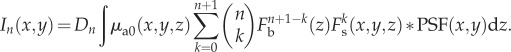
The operating principle of LSF–PIM is shown in figure 1c. Upon light sheet excitation, the light intensity measured by a wide-field microscope is an integration of the fluorescence emitted from all depths:

2.1

where C is a constant, μ_a is the absorption coefficient of the fluorophore, F_b represents the ballistic excitation (i.e. unscattered photon) fluence in J m⁻², F_s represents the scattered excitation (i.e. scattered photon) fluence, PSF_z is the point-spread-function (PSF) of the fluorescence imaging system at depth z, and the operator asterisk denotes two-dimensional convolution in the x − y plane. The imaging FOV is determined by the excitation beam's depth of focus, d, which is approximated by

2.2

Here, λ is the excitation laser wavelength. Within this FOV, the ballistic excitation fluence is assumed to be uniform along the x- and y-directions. Equation (2.1) can be simplified to

2.3

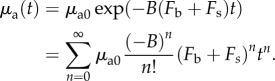
In fluorescence microscopy, photobleaching occurs when excited electrons are trapped in a relatively long-lived triplet state. Compared with the singlet–singlet transition, the forbidden triplet–singlet transition provides a fluorophore a much longer time to undergo irreversible chemical reactions with the environment [9]. The photobleaching reduces the local absorption coefficient, resulting in an exponential decay with time:

2.4

Here, t is time, is the initial absorption coefficient of the fluorophore and k is the photobleaching rate. The photobleaching rate, k, is a function of the total excitation fluence [10]. For one-photon excitation, the relation is described by

2.5

where B is a constant. By substituting equation (2.5) into (2.4), followed by Taylor expansion with respect to time t, we obtain

2.6

Substituting equation (2.6) into (2.3) gives

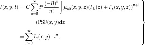2.7

where

2.8

and . Here, I_n(x,y) is the coefficient associated with tⁿ and can be derived from the polynomial fitting of I(x, y, t).

Binomial expansion of the term in equation (2.8) gives

2.9

Because outside the optical section ( or , ) and within the optical section (), the cross terms in equation (2.9) are negligible. Equation (2.9) becomes

2.10

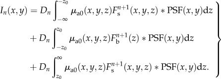
The ballistic fluence reaches a maximum at the depth z = 0. Rearranging equation (2.10) yields

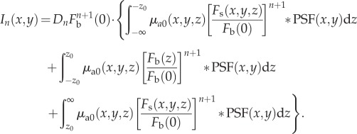2.11

In the case that 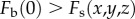at all depths, the first and third terms in equation (2.11) approach zero when . Therefore, for a high-order PIM component, the background signals associated with scattered excitation fluence (the first and third terms in equation (2.11)) are suppressed. Additionally, the optical section associated with ballistic excitation fluence (the second term in equation (2.11)) is also reduced by a factor of in thickness (figure 1d,e).

To show that LSF–PIM can decrease optical sectioning thickness while maintaining a relatively large FOV, we computed the effective excitation volume by tracking the wavefront using the Fourier optical transformation [11]. With an objective of NA = 0.1 for light sheet excitation (λ = 550 nm), the derived cross-sectional (x − z) images associated with conventional LSFM, LSF–PIM (I₁) and LSF–PIM (I₄) are shown in figure 2a–c, respectively. The signal intensities along the dashed line in figure 2a–c are shown in figure 2d. The full width at half maximum (FWHM) of the corresponding axial responses is 2.4, 1.7 and 1.1 μm, respectively. As expected, a higher-order LSF–PIM signal results in a thinner optical section. For comparison, we also simulated the effective excitation volume with an objective of NA = 0.25 for light sheet excitation (figure 2e). In this case, the light sheet's thickness (1.1 μm) approaches that in LSF–PIM (I₄); however, the drawback lies in a much shorter sheet extent along the x-axis. Consequently, provided that the sectioning thickness is comparable, LSM–PIM is superior to conventional LSFM in terms of imaging FOV.

Figure 2.

Simulated effective excitation volume in (a) LSFM with an excitation objective of NA = 0.1, (b) the corresponding first-order LSF–PIM and (c) fourth-order LSF–PIM. (d) Comparison of signal intensities along the dashed line in (a–c). (e) Simulated effective excitation volume in LSFM with an excitation objective of NA = 0.25. The optical sectioning thickness in (c) is comparable to that in (e), yet with a six times larger (in diameter) imaging FOV. (Online version in colour.)

3. Results and discussion

To demonstrate LSF–PIM experimentally, we first imaged a phantom sample consisting of red fluorescent beads (diameter, 0.9 μm; maximum emission wavelength, 600 nm) uniformly mixed and sealed in gelatin. The sample was excited by a 532 nm continuous wave (CW) laser and imaged on a custom-built LSF microscope (Material and methods). With an objective of NA = 0.1 for light-sheet excitation, a conventional LSFM image was captured and is shown in figure 3a. The imaging depth is approximately 500 μm below the sample surface. Owing to the relatively thick optical section and light scattering, most in-focus fluorescent beads are obscured by out-of-focus light. By contrast, after measuring 100 time-lapse fluorescence images (0.1 s frame integration time), we calculated the LSF–PIM (I₂, I₄) images, shown in figure 3b,c, respectively. Three corresponding areas from figure 3a–c are zoomed in for further comparison. The fluorescent beads are much more distinguishable in figure 3b,c because of the much thinner effective optical section. Additionally, the signal intensities across the dashed line in figure 3a–c are compared. The results (figure 3d) indicate that the higher-order PIM component leads to higher image contrast.

Figure 3.

Light-sheet fluorescence imaging of red fluorescent beads (0.9 μm in diameter) mixed in gelatin. (a) Conventional LSFM image. (b) LSF–PIM (I₂) image. (c) LSF–PIM (I₄) image. (d) Comparison of signal intensities across the dashed line in (a–c). (Online version in colour.)

Next, we imaged a zebrafish embryo 6 days post-fertilization (dpf) in vivo with LSF–PIM. In the transgenic embryo, the myelin basic protein (mbp) promoter drives expression of mcherry throughout the nervous system [12,13], and the spinal cord was imaged. The light sheet's incident direction (green arrow) was perpendicular to the spinal cord axis (figure 4a). Imaging a 6 dpf or older fish in vivo is generally considered as a challenge for conventional LSFM owing to light scattering [5]. Here, for that reason, the conventional LSFM image (figure 4b) suffers from severe blurring. By contrast, in the corresponding LSF–PIM image (figure 4c), because most out-of-focus light is rejected, the sample's spinal cord is clearly seen. To provide a gold standard, the same embryo was also imaged by a confocal fluorescence microscope (Material and methods). The captured cross-sectional image of the spinal cord is shown in figure 4d. The signal intensities across the dashed lines in figure 4b–d were compared (figure 4e). The result implies that while the conventional LSFM fails to provide the contrast, the LSM–PIM accurately resembles the gold-standard image. The image contrast was improved approximately six times by using LSM–PIM. In addition, we also acquired a three-dimensional image of the embryo's spinal cord by scanning the sample along the z-axis (figure 4f). The recovery of the spinal cord in three dimensions from a strong fluorescence background substantiates LSF–PIM's superior imaging capability through a scattering medium.

Figure 4.

LSF–PIM imaging of a 6 dpf tg(mbp:mcherry-caax) zebrafish embryo. (a) Bright-field transmission image. In the transgenic embryo, the myelin basic protein (mbp) promoter drives expression of mcherry throughout the nervous system [12,13], and the spinal cord is imaged. The light sheet's incident direction (indicated by the green arrow) is along the y-axis. (b) Conventional LSFM image (0.1 s frame integration time). (c) LSF–PIM image (I₁₀). (d) Gold-standard confocal image. (e) Comparison of signal intensities along the dashed line in (b–d). CM, confocal microscopy. (f) Three-dimensional image of the spinal cord acquired by LSF–PIM (I₁₀). (Online version in colour.)

The contrast enhancement by LSF–PIM is accomplished at the expense of an increased acquisition time. The accuracy of fitting time-lapse fluorescence decay into a polynomial function is highly dependent on the number of temporal samplings and the signal-to-noise ratio (SNR). Thus, to extract the higher-order PIM components, more temporal samplings are needed and more photons must be collected at each sampling point. Depending on the sample and application, one can determine an optimal experimental setting to achieve the desired image contrast and temporal resolution. Here, to extract the PIM component I₁₀ (figure 4c), a total of 200 time-lapse images was measured with a 0.1 s frame integration time.

4. Conclusion

In summary, we presented a nonlinear LSF imaging approach based on PIM. Compared with conventional LSFM, our method features two advantages: on the one hand, it simultaneously achieves a large imaging FOV and a thin optical section; on the other hand, it effectively removes the scattering-induced background, thereby allowing much deeper penetration into a thick medium. We demonstrated the deep imaging capability of LSF–PIM by imaging a scattering phantom and a 6 dpf fish embryo in vivo—while conventional LSFM showed almost no contrast between the in-focus signals and background, LSF–PIM clearly resolved the sample features and closely resembled the gold standard. Owing to its easy implementation and superior imaging capability, LSF–PIM is expected to open new areas of investigation in studies involving relatively large and non-transparent living organisms.

5. Material and methods

5.1. Preparation of the phantom sample

Gelatin was dissolved in warm deionized water to form a 10% solution, then uniformly mixed with red fluorescent beads (R900, Fisher Scientific; average diameter, 0.9 μm). The mixture was cooled to 4°C to form a gel.

5.2. Zebrafish husbandry

Zebrafish embryos were raised at 28.5°C and staged according to published methods [14]. All animal work was performed in compliance with Washington University's institutional animal protocols. tg(mbp:mcherry-caax) zebrafish were a kind gift of Dr David Lyons (University of Edinburgh) [12,13]. Larvae were raised in 0.0045% phenylthiourea in embryo medium to prevent the formation of melanin pigments. For visualization, larvae were anaesthetized with tricaine methanesulfonate and immobilized in low melt agarose.

5.3. Light-sheet fluorescence microscopy

A light-sheet microscope was built for fluorescence imaging (see electronic supplementary material, figure S1). A CW laser (diameter, 2 mm; wavelength, 532 nm) is used for fluorescence excitation. The excitation strength is adjusted by a combination of a 1/2 λ waveplate (AHWP05M-600, Thorlabs) and a polarizing beam splitter (PBS101, Thorlabs). The excitation laser is focused into a line by a cylindrical lens of 50 mm focal length (LJ1695RM-A, Thorlabs). Then, the laser line image is relayed to the back aperture of a four times microscope objective (Plan Fluorite, Nikon) with NA = 0.1 through a 4-f telecentric imaging system consisting of a lens of 25 mm focal length (LA1951-A, Thorlabs) and a lens of 100 mm focal length (LA1509-A, Thorlabs). The fluorescence is collected by a 10× microscope objective (Plan Fluorite, Nikon) with NA = 0.3, filtered by an emission filter (central wavelength, 559 nm; bandwidth, 34 nm), and imaged by a CCD camera (ORCA-R², Hamamatsu). The FWHM of the point-spread-function on the fluorescence imaging side is 12.2 μm, and is sampled by 2 × 2 camera pixels (pixel size, 6.45 μm). To achieve volumetric imaging, the sample is scanned along the z-axis with a step size of 50 μm.

5.4. Photobleaching imprinting microscopy and image processing

The PIM is conducted by measuring time-lapse fluorescence decay, followed by polynomial fitting and extraction of high-order, fluence-dependent coefficients. To make the PIM image reconstruction algorithm easily accessible to the biological research community, we implemented it as an open-source plugin for the widely used ImageJ software (http://rsb.info.nih.gov/ij/). The LSF–PIM ImageJ plugin is freely available at http://code.google.com/p/lsf-pim.

5.5. Confocal fluorescence microscopy

The gold-standard image shown in figure 4d was captured on a commercial confocal laser scanning fluorescence microscope (FV1000, Olympus) with 1 s acquisition time. We used a 40× microscope objective (Plan Fluorite, NA = 0.75) to excite the fluorophore and collect fluorescence, and an RFP filter set (Olympus) to separate fluorescence from excitation light. An optimal pinhole size was automatically chosen by the microscope to balance the in-focus SNR and optical sectioning thickness. To increase the image SNR, a Kalman filter was applied during data acquisition.

References

- 1.Santi PA. 2011. Light sheet fluorescence microscopy: a review. J. Histochem. Cytochem. 59, 129–138. ( 10.1369/0022155410394857) [DOI] [PMC free article] [PubMed] [Google Scholar]
- 2.Reynaud EG, Krzic U, Greger K, Stelzer EHK. 2008. Light sheet-based fluorescence microscopy: more dimensions, more photons, and less photodamage. Hfsp J. 2, 266–275. ( 10.2976/1.2974980) [DOI] [PMC free article] [PubMed] [Google Scholar]
- 3.Voie AH, Burns DH, Spelman FA. 1993. Orthogonal-plane fluorescence optical sectioning: three-dimensional imaging of macroscopic biological specimens. J. Microsc. 170, 229–236. ( 10.1111/j.1365-2818.1993.tb03346.x) [DOI] [PubMed] [Google Scholar]
- 4.Fahrbach FO, Gurchenkov V, Alessandri K, Nassoy P, Rohrbach A. 2013. Self-reconstructing sectioned Bessel beams offer submicron optical sectioning for large fields of view in light-sheet microscopy. Opt. Express 21, 11 425–11 440. ( 10.1364/OE.21.011425) [DOI] [PubMed] [Google Scholar]
- 5.Keller PJ, Schmidt AD, Santella A, Khairy K, Bao ZR, Wittbrodt J, Stelzer EHK. 2010. Fast, high-contrast imaging of animal development with scanned light sheet-based structured-illumination microscopy. Nat. Methods 7, U637–U655. ( 10.1038/nmeth.1476) [DOI] [PMC free article] [PubMed] [Google Scholar]
- 6.Mertz J, Kim J. 2010. Scanning light-sheet microscopy in the whole mouse brain with HiLo background rejection. J. Biomed. Opt. 15, 016027 ( 10.1117/1.3324890) [DOI] [PMC free article] [PubMed] [Google Scholar]
- 7.Cella Zanacchi F, Lavagnino Z, Faretta M, Furia L, Diaspro A. 2013. Light-sheet confined super-resolution using two-photon photoactivation. PLoS ONE 8, e67667 ( 10.1371/journal.pone.0067667) [DOI] [PMC free article] [PubMed] [Google Scholar]
- 8.Keller PJ, Dodt HU. 2012. Light sheet microscopy of living or cleared specimens. Curr. Opin. Neurobiol. 22, 138–143. ( 10.1016/j.conb.2011.08.003) [DOI] [PubMed] [Google Scholar]
- 9.Tsien RY, Ernst L, Waggoner A. 2006. Fluorophores for confocal microscopy: photophysics and photochemistry. In Handbook of biological confocal microscopy (ed. Pawley JB.), pp. 338–348 Berlin, Germany: Springer. [Google Scholar]
- 10.Patterson GH, Piston DW. 2000. Photobleaching in two-photon excitation microscopy. Biophys. J. 78, 2159–2162. ( 10.1016/S0006-3495(00)76762-2) [DOI] [PMC free article] [PubMed] [Google Scholar]
- 11.Barrett HH, Myers KJ. 2004. Foundations of image science. Wiley Series in Pure and Applied Optics. Hoboken, NJ: Wiley-Interscience. [Google Scholar]
- 12.Czopka T, Ffrench-Constant C, Lyons DA. 2013. Individual oligodendrocytes have only a few hours in which to generate new myelin sheaths in vivo. Dev. Cell 25, 599–609. ( 10.1016/j.devcel.2013.05.013) [DOI] [PMC free article] [PubMed] [Google Scholar]
- 13.Almeida RG, Czopka T, Ffrench-Constant C, Lyons DA. 2011. Individual axons regulate the myelinating potential of single oligodendrocytes in vivo. Development 138, 4443–4450. ( 10.1242/dev.071001) [DOI] [PMC free article] [PubMed] [Google Scholar]
- 14.Kimmel CB, Ballard WW, Kimmel SR, Ullmann B, Schilling TF. 1995. Stages of embryonic development of the zebrafish. Dev. Dyn. 203, 253–310. ( 10.1002/aja.1002030302) [DOI] [PubMed] [Google Scholar]