Learning an Internal Dynamics Model from Control Demonstration

Abstract

Much work in optimal control and inverse control has assumed that the controller has perfect knowledge of plant dynamics. However, if the controller is a human or animal subject, the subject’s internal dynamics model may differ from the true plant dynamics. Here, we consider the problem of learning the subject’s internal model from demonstrations of control and knowledge of task goals. Due to sensory feedback delay, the subject uses an internal model to generate an internal prediction of the current plant state, which may differ from the actual plant state. We develop a probabilistic framework and exact EM algorithm to jointly estimate the internal model, internal state trajectories, and feedback delay. We applied this framework to demonstrations by a nonhuman primate of brain-machine interface (BMI) control. We discovered that the subject’s internal model deviated from the true BMI plant dynamics and provided significantly better explanation of the recorded neural control signals than did the true plant dynamics.

1. Introduction

Inverse optimal control (IOC) and inverse reinforcement learning (IRL) aim to identify a cost function from demonstrations of successful control (Boyd et al., 1994; Schaal, 1999; Ng & Russell, 2000; Abbeel & Ng, 2004; Ratliff et al., 2006; Coates et al., 2008; Ziebart et al., 2008). These approaches typically require a model of the plant dynamics, which enables prediction of future states given the current state and control input. In previous work, it has been assumed that the controller’s internal belief about the plant dynamics matches the actual plant dynamics. However, when the controller is a human or animal subject, this internal belief may differ from the actual plant dynamics (Crapse & Sommer, 2008), especially if the subject has limited experience driving the plant. This mismatch can exist even when demonstrated control is proficient (e.g., the implemented control strategy may be only locally optimal). Because the plant dynamics and cost function jointly determine the optimal control policy, an incorrect assumption about the dynamics model can lead to misestimation of the cost function via IOC or IRL.

Ideally, we would like to use demonstrated control to learn both the subject’s internal model of the plant dynamics and the cost function together. This joint estimation is difficult, so previous work has focused on learning the cost function while assuming known plant dynamics. Here, we present and solve the complementary problem of learning the subject’s internal model of the plant dynamics while assuming knowledge of the task goals. This problem is challenging because at each control decision, the subject must generate an internal estimate of the current plant state based on delayed sensory feedback (Miall & Wolpert, 1996), and we cannot directly observe these internal state estimates.

We introduce a probabilistic internal model estimation (IME) framework through which inference and learning provide a solution to the current problem in the setting of linear-Gaussian internal model dynamics and quadratic cost functions. In IME, the subject’s internal model of the plant dynamics defines trajectories of latent variables representing the subject’s moment-by-moment internal estimates of the plant state. We assume knowledge of the control signals sent by the subject, the plant state feedback available to the subject, and target states to which the subject intends to drive the plant during control. Importantly, we make no assumption that the subject’s internal dynamics model should match the true plant dynamics.

Beyond the algorithmic advance, the ability to extract a subject’s internal model has many potential applications in neuroscience and human-in-the-loop control. Access to a subject’s internal model could provide a means for tracking and encouraging skill acquisition in complex tasks, including brain-machine interface (BMI) control, telerobotic surgery or remote control of unmanned-aerial vehicles. In this work we apply the developed methods toward demonstrations of BMI cursor control. BMIs have been developed to assist disabled patients by translating neural activity into control signals for a prosthetic limb or computer cursor (Green & Kalaska, 2011). BMI control is an acquired skill, akin to driving a car or helicopter. Previous studies have shown that subjects improve BMI control performance over time (Taylor et al., 2002; Ganguly et al., 2011). This improvement is likely a result of the subject refining an internal model of the BMI plant dynamics through experience. Access to the subject’s internal model of the BMI, through the methods we develop here, may inform the design of future BMI systems and may provide neuroscientists with novel tools for investigating the neural basis of feedback motor control and motor learning.

We begin Section 2 by formalizing the internal model estimation problem. In Section 3 we propose a probabilistic framework for solving the internal model estimation problem. Section 4 details the validation of the framework through application to real neural data underlying BMI control of a computer cursor.

2. Problem Formulation

A standard control model takes the following form:

$$\mathbf{\text{Dynamics}}\mathbf{:}{\mathbf{x}}_{\mathrm{t}+1}={\mathit{f}}_{\mathit{1}}({\mathbf{x}}_{\mathrm{t}},{\mathbf{u}}_{\mathrm{t}})$$ (1)

$$\mathbf{\text{Cost}}\mathbf{:}\mathit{J}(\{{\mathbf{x}}_{\mathrm{t}}\},\{{\mathbf{u}}_{\mathrm{t}}\})$$ (2)

where f₁ represents the subject’s belief about the plant dynamics, x_t ∈ ℝⁿ is the subject’s belief of the plant state at timestep t, u_t ∈ ℝ^m is the control input issued at timestep t, and J is the cost function that encodes task goals and control effort. We distinguish the subject’s internal model of the plant dynamics, f₁, from the actual plant dynamics, f₂:

$${\mathbf{y}}_{\mathrm{t}+1}=f_2({\mathbf{y}}_{\mathrm{t}},{\mathbf{u}}_{\mathrm{t}})$$ (3)

where y_t ∈ ℝ^p is the actual plant state at timestep t.

Due to sensory feedback delay, the feedback available at timestep t represents the plant state at timestep t − τ, where τ is the feedback delay. To predict the current plant state, the subject can use f₁ as a forward model, propagating y_t−τ (or a noise-corrupted function of it) forward in time using knowledge of the plant dynamics and previously issued controls u_t−τ, …, u_t−1. In general, the subject’s internal beliefs {x_t} may be inconsistent with the actual plant states {y_t} due to differences between f₁ and f₂ and due to sensory noise.

The problem we seek to solve is:

$$\begin{gathered} \mathbf{\text{Given}}\mathbf{:}\{{\mathbf{y}}_{\mathrm{t}}\},\{{\mathbf{u}}_{\mathrm{t}}\},\mathit{J} \\ \mathbf{\text{Estimate}}\mathbf{:}{\mathit{f}}_{\mathit{1}},\{{\mathbf{x}}_{\mathrm{t}}\},\tau \end{gathered}$$

That is, given trajectories of actual plant state and control input, and assuming a cost function, we seek to estimate the subject’s internal model of the plant dynamics, the subject’s internal estimates of plant state, and the sensory feedback delay.

In the remainder of this paper, we focus on the case where f₁ is linear-Gaussian and J is quadratic over the internal states, in analogy to the well-studied linear-quadratic regulator (Anderson & Moore, 1990). These choices allow us to derive an approximation-free algorithm to solve the internal model estimation problem.

3. Probabilistic framework for internal model estimation

The IME probabilistic model is as follows:

$${\mathbf{x}}_{\mathrm{t}-\tau }^{\mathrm{t}}|{\mathbf{y}}_{\mathrm{t}-\tau }~𝒩(\mathbf{H}{\mathbf{y}}_{\mathrm{t}-\tau ,}{\mathbf{W}}_0)$$ (4)

$${\mathbf{x}}_{\mathrm{k}+1}^{\mathrm{t}}|{\mathbf{x}}_{\mathrm{k}}^{\mathrm{t}},{\mathbf{u}}_{\mathrm{k}}~𝒩(\mathbf{A}{\mathbf{x}}_{\mathrm{k}}^{\mathrm{t}}+\mathbf{B}{\mathbf{u}}_{\mathrm{k}}+{\mathbf{b}}_{0,}\mathbf{W})$$ (5)

$${\mathbf{G}}_{\mathrm{t}}|{\mathbf{x}}_{\mathrm{t}+1}^{\mathrm{t}}~𝒩({\mathbf{C}}_{\mathrm{t}}{\mathbf{x}}_{\mathrm{t}+1}^{\mathrm{t}},\mathbf{V})$$ (6)

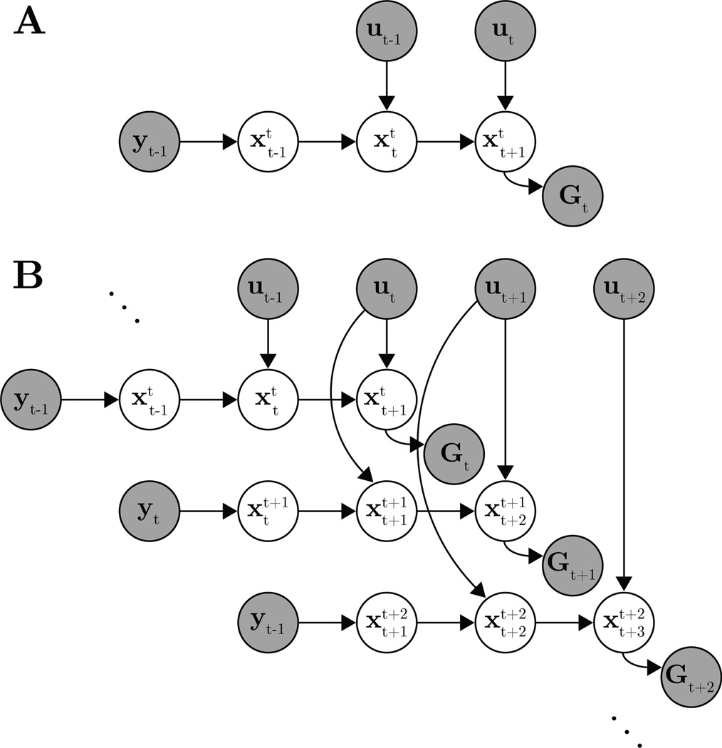
At timestep t ∈ {1,…, T}, y_t ∈ ℝ^p is the actual plant state, ${\mathbf{x}}_{\mathrm{k}}^{\mathrm{t}}\in {ℝ}^{\mathrm{n}}$ is the subject’s internal estimate of the timestep k ∈ {t−τ, …, t+1} plant state (see below for detailed explanation), u_t ∈ ℝ^m is the subject’s control input, and G_t ∈ ℝ^q represents control goals. The parameters are the feedback matrix H ∈ ℝ^n×p, the subject’s internal model parameters {A ∈ ℝ^n×n, B ∈ ℝ^n×m, b₀ ∈ ℝⁿ}, the cost matrices C_t ∈ ℝ^q×n, noise covariance matrices {W₀ ∈ ℝ^n×n, W ∈ ℝ^n×n, V ∈ ℝ^q×q}, and the sensory feedback delay τ ∈ ℤ⁺. The IME graphical model for a single timestep feedback delay (τ = 1) is shown in Fig. 1.

Figure 1.

IME graphical model with a single timestep feedback delay (τ = 1). Observed variables are indicated as shaded nodes, and unshaded nodes are latent variables. (A) Timestep t slice of IME. Delayed sensory feedback of plant state, y_t−1, and previously issued control input, u_t−1, propagate through the subject’s internal dynamics model to generate internal estimates of plant state, ${\mathbf{x}}_{\mathrm{t}-1}^{\mathrm{t}}$ and ${\mathbf{x}}_{\mathrm{t}}^{\mathrm{t}}$. With belief ${\mathbf{x}}_{\mathrm{t}}^{\mathrm{t}}$ of the current plant state, the subject generates a new control signal, u_t. The internal model predicts the resulting future state, ${\mathbf{x}}_{\mathrm{t}+1}^{\mathrm{t}}$, which should agree with the current task goal, G_t. (B) The full IME graphical model. The timestep t slice from (A) is embedded in the upper left corner.

Due to sensory delays, the plant state feedback available at timestep t is outdated by τ timesteps. Accordingly, (4) defines the subject’s noisy, partial observation of delayed plant state feedback. Sitting at timestep t, the subject uses this feedback, y_t−τ, to form an internal estimate, ${\mathbf{x}}_{\mathrm{t}-\tau }^{\mathrm{t}}$, of the timestep t −τ plant state. The noise covariance W₀ accounts for sensory noise.

We define the subject’s internal dynamics model in (5) to be a Gaussian linear-dynamical system that propagates the subject’s internal estimates of plant state given control input. At timestep t, the subject makes internal estimates, ${\mathbf{x}}_{\mathrm{k}}^{\mathrm{t}}$, of the past (k = t−τ,…, t−1), current (k = t), and future (k = t + 1) plant states. This timestep t internal state chain (Fig. 1A) corresponds to a row of latent states in the IME graphical model (Fig. 1B). The state chain begins with ${\mathbf{x}}_{\mathrm{t}-\tau }^{\mathrm{t}}$, the subject’s internal belief about the plant state feedback, y_t−τ. Subsequent internal state estimates, $\{{\mathbf{x}}_{\mathrm{t}-\tau +1}^{\mathrm{t}},\dots ,{\mathbf{x}}_{\mathrm{t}+1}^{\mathrm{t}}\}$, may be inconsistent with the true plant states, {y_t−τ+1,…, y_t+1}, because i) sensory feedback is not yet available for these timesteps, and ii) there may be mismatch between the subject’s internal model (5) and the true plant dynamics (3). Internal state transitions not explained by the internal model are accounted for by the noise covariance, W. At timestep t+1, the subject receives new plant feedback, y_t−τ+1, and generates revised internal estimates, $\{{\mathbf{x}}_{\mathrm{t}-\tau +1}^{\mathrm{t}+1},\dots ,{\mathbf{x}}_{\mathrm{t}+2}^{\mathrm{t}+1}\}$, corresponding to a new row of latent states in the graphical model. The variables, ${\mathbf{x}}_{\mathrm{k}}^{\mathrm{t}}$, where we fix k and vary t ∈ {k − 1,…, k + τ}, correspond to a column of latent states in the graphical model and represent successive revisions of the subject’s beliefs about the timestep k plant state, given the sensory feedback available at timestep t. Note that (5) is the IME instantiation of (1).

In (6), we encode the subject’s cost function. At timestep t, the subject determines the next control signal to send, u_t, which the subject’s internal model predicts will drive the plant to state ${\mathbf{x}}_{\mathrm{t}+1}^{\mathrm{t}}$. The cost matrix, C_t, relates this internal state estimate to the given control goals, G_t. Depending on the application, C_t may be fully specified in advance, or may contain parameters to be learned. For example, in a trajectory tracking task, the G_t might encode the (known) desired trajectory, and C_t might simply extract appropriate components of the subject’s internal estimate of the upcoming plant state, ${\mathbf{x}}_{\mathrm{t}+1}^{\mathrm{t}}$. Alternatively, C_t might compute linear functions of feature counts (Ng & Russell, 2000; Abbeel & Ng, 2004) from the subject’s internal state estimates. In Section 4 we describe an application in which the G_t are constant across timesteps and represent a control goal to be attained by some arbitrary time in the future. In this application, we use C_t to extract the extent to which the subject is on track to achieve the goal state. Note that (6) relates to (2), but does not incorporate control effort. We focus the scope of this work to problems where either i) the cost function is dominated by the state cost, or ii) we can structure the C_t in (6) to account for an unknown control cost (see Section 4 for an example).

3.1. Model Fitting

In model fitting, we treat actual plant states, {y_t}, control inputs, {u_t}, and task goals, {G_t}, as observed variables. We treat the internal state estimates, $\{{\mathbf{x}}_{\mathrm{t}-\tau }^{\mathrm{t}},\dots ,{\mathbf{x}}_{\mathrm{t}+1}^{\mathrm{t}}\}$, as unobserved latent variables. We seek the model parameters, H, W₀, A, B, b₀, W, {C_t}¹, V, and τ, that maximize P({G_t}|{y_t}, {u_t}), the likelihood of the control goals under the distribution induced by (4)–(6).

We derived an exact expectation-maximization (EM) algorithm (Dempster et al., 1977) for a specified feed-back delay, τ (see APPENDIX). In the E-step, we infer posterior distributions over the latent variables, $\mathrm{P}(\{{\mathbf{x}}_{\mathrm{t}-\tau }^{\mathrm{t}},\dots ,{\mathbf{x}}_{\mathrm{t}+1}^{\mathrm{t}}\}|\{{\mathbf{y}}_{\mathrm{t}}\},\{{\mathbf{u}}_{\mathrm{t}}\},\{{\mathbf{G}}_{\mathrm{t}}\})$, using the current parameter estimates. In the M-step, we update model parameters given the posterior latent variable distributions. Since the relationships in (4)–(6) are linear-Gaussian, all latent and observed variables are jointly Gaussian. Additionally, given all control inputs, an internal state chain for one timestep is conditionally independent of the internal state chains for all other timesteps

$${\mathbf{x}}_{{\mathrm{t}}_1-\tau }^{{\mathrm{t}}_1},\dots ,{\mathbf{x}}_{{\mathrm{t}}_1+1}^{{\mathrm{t}}_1}\perp {\mathbf{x}}_{{\mathrm{t}}_2-\tau }^{{\mathrm{t}}_2},\dots ,{\mathbf{x}}_{{\mathrm{t}}_2+1}^{{\mathrm{t}}_2}|\{{\mathbf{u}}_{\mathrm{t}}\}$$ (7)

where t₁ ≠ t₂. These properties of IME enable an exact and efficient E-step update to the posterior latent variable distributions, and closed-form M-step parameter updates.

To identify the feedback delay, τ, we fit IME across a sequence of τ values. As τ increases, the number of parameters remains fixed, and thus increasing τ does not lead to overfitting. For this reason we can simply choose τ_ML to be the τ whose corresponding IME fit gives the highest training data likelihood, P({G_t}|{y_t}, {u_t}).

4. Internal model estimation from brain-machine interface control

We demonstrate an application of the IME framework to closed-loop BMI cursor control. A BMI system can be viewed as a feedback control system, whereby a human or animal subject (controller) generates neural activity (control signal) to drive a computer cursor (plant). The experimenter defines the mapping from recorded neural activity to cursor movements (i.e., the actual plant dynamics). The experimenter also defines the task goals in each trial by displaying a visual target to which the subject is instructed to drive the BMI cursor. At any moment in time, the subject does not know the current cursor position due to visual feedback delays in the nervous system, and therefore must choose a control signal to issue based on visual feedback of an outdated cursor position. We assume that the subject always intends to drive the cursor straight to the target from an internal estimate of the current cursor position. We seek to use IME to estimate the subject’s internal model of the BMI cursor dynamics along with the subject’s timestep-by-timestep internal estimates of the current BMI cursor position.

Previous studies have provided behavioral and neurophysiological evidence that subjects use internal models during motor control (Crapse & Sommer, 2008). In the context of BMI, subjects need to learn to control the cursor, which likely involves refining the internal model with practice controlling the BMI.

4.1. BMI experiments

A 96-channel Utah electrode array was implanted in motor cortex of a Rhesus monkey. In each of 36 experimental sessions, we simultaneously recorded from tens (26 ± 3.44) of neurons, and spike counts were taken in Δt = 33 ms non-overlapping bins. Two-dimensional cursor velocity was linearly decoded from recorded spike counts, and cursor positions were updated according to

$${\mathbf{y}}_{\mathrm{t}+1}={\mathbf{y}}_{\mathrm{t}}+\mathit{\beta }{\mathbf{ũ}}_{\mathrm{t}}+{\beta }_0$$ (8)

$${\mathbf{ũ}}_{\mathrm{t}}=\frac{1}{5}\sum _{k=0}^4{\mathbf{u}}_{\mathrm{t}-\mathrm{k}}$$ (9)

where y_t ∈ ℝ² is the cursor position displayed at timestep t, u_t ∈ ℝ^m is the raw spike count vector across m simultaneously recorded neuronal units at timestep t, and ũ_t ∈ ℝ^m is the vector mean spike count over the past 5 timesteps. The decoding parameters β ∈ ℝ^2×m and β₀ ∈ ℝ² were determined via the population vector algorithm (Georgopoulos et al., 1983). Note that (8) describes the actual dynamics of the BMI cursor, corresponding to (3).

In each experimental trial, the subject modulated neural activity to drive the BMI cursor (radius, 8 mm) to a target (radius, 8 mm) that appeared on the perimeter of a circular workspace (radius, 85 mm). A trial was deemed successful and terminated as soon as the cursor visibly overlapped with the target for 50 ms. A trial was deemed a failure if the subject did not acquire the target within 2 s. The subject typically failed less than 5% of trials. Experimental details were previously described in Chase et al. (2012).

4.2. IME formulation for BMI control

The specific IME formulation we applied to the BMI control data is as follows:

$${\mathbf{x}}_{\mathrm{t}-\tau }^{\mathrm{t}}={\mathbf{y}}_{\mathrm{t}-\tau }$$ (10)

$${\mathbf{x}}_{\mathrm{k}+1}^{\mathrm{t}}|{\mathbf{x}}_{\mathrm{k}}^{\mathrm{t}},{\mathbf{u}}_{\mathrm{k}}~𝒩(\mathbf{A}{\mathbf{x}}_{\mathrm{k}}^{\mathrm{t}}+\mathbf{B}{\mathbf{u}}_{\mathrm{k}}+{\mathbf{b}}_0,{\sigma }_{\mathbf{x}}^2\mathbf{I})$$ (11)

$${\mathbf{G}}_{\mathrm{t}}|{\mathbf{x}}_{\mathrm{t}}^{\mathrm{t}},{\mathbf{x}}_{\mathrm{t}+1}^{\mathrm{t}}~𝒩({\mathbf{x}}_{\mathrm{t}+1}^{\mathrm{t}}+{\mathrm{c}}_{\mathrm{t}}({\mathbf{x}}_{\mathrm{t}+1}^{\mathrm{t}}-{\mathbf{x}}_{\mathrm{t}}^{\mathrm{t}}),{\sigma }_{\mathbf{G}}^2\mathbf{I})$$ (12)

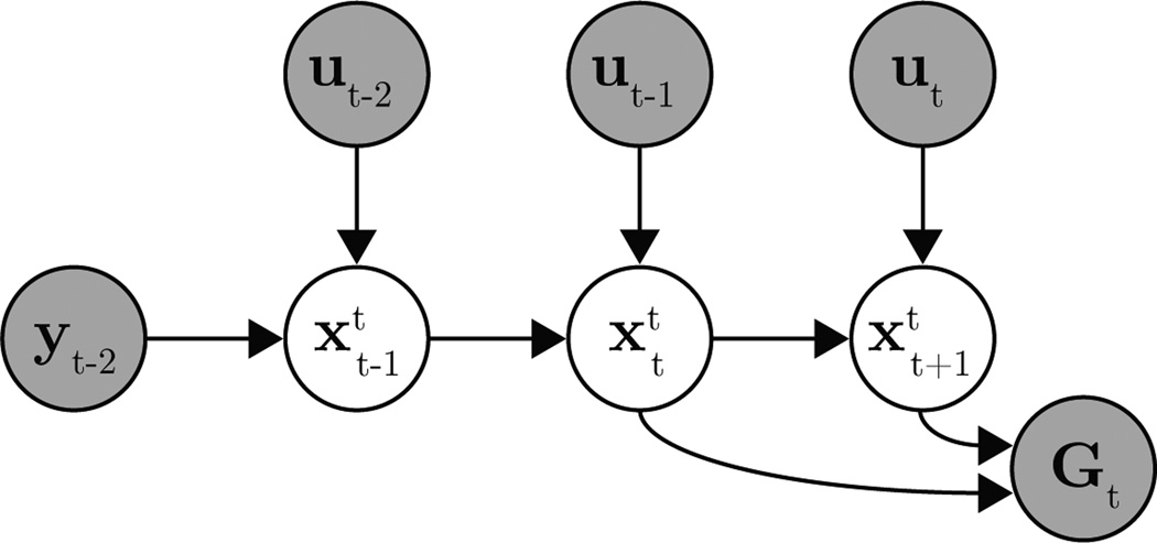
where (10)–(12) are specific instances of (4)–(6). A single-timestep slice of this IME graphical model is shown in Fig. 2.

Figure 2.

Single-timestep slice of a two-timestep feedback delay (τ = 2) IME graphical model, as used in the BMI application.

Since the BMI experiments used a position-only state, we define the subject’s internal state estimates to reside in the same 2-dimensional position space to allow for interpretable A, B, b₀, and $\{{\mathbf{x}}_{\mathrm{k}}^{\mathrm{t}}\}$. For simplicity, we assume the BMI subject has noiseless access to delayed visual feedback of cursor position. These choices are formalized in (10), where ${\mathbf{x}}_{\mathrm{t}-\tau }^{\mathrm{t}}\in {ℝ}^2$ is the internal estimate made by the subject at timestep t of the BMI cursor position at timestep t−τ, and y_t−τ∈ ℝ² is the actual BMI cursor position at timestep t − τ.

In (11), ${\mathbf{x}}_{\mathrm{k}}^{\mathrm{t}}\in {ℝ}^2$ is the subject’s internal estimate made at timestep t of the timestep k ∈ {t−τ, …, t+1} cursor position, and the control input u_t ∈ ℝ^m is neural activity recorded at timestep t, as defined in Section 4.1. Note that the form of the subject’s internal dynamics model in (11) matches the form of the actual cursor dynamics from (8), allowing for direct comparison between the two.

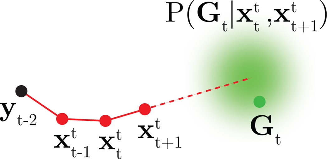
The cost function in (12) encodes the subject’s intention to drive the cursor straight toward the current visual target position, G_t ∈ ℝ², from the subject’s up-to-date estimate of cursor position, ${\mathbf{x}}_{\mathrm{t}}^{\mathrm{t}}$, as illustrated in Fig. 3. Within a particular BMI trial, all {G_t} take the same value. The straight-to-target aiming intention is implemented by the neural control input, u_t, which the subject’s internal model predicts will bring the cursor to position ${\mathbf{x}}_{\mathrm{t}+1}^{\mathrm{t}}$. The mean of the distribution in (12) lies on the line defined by the two points, ${\mathbf{x}}_{\mathrm{t}}^{\mathrm{t}}$ and ${\mathbf{x}}_{\mathrm{t}+1}^{\mathrm{t}}$. The length of the line segment between ${\mathbf{x}}_{\mathrm{t}+1}^{\mathrm{t}}$ and G_t is controlled by c_t, which is determined by the data. The noise variance, ${\sigma }_{\mathbf{G}}^2$, accounts for motor commands that deviate from straight-to-target aiming.

Figure 3.

Task goals encoded by the IME probabilistic model. For illustration, we consider a two-timestep visual feedback delay. At timestep t, the subject’s internal estimate of the cursor position two timesteps ago matches the actual cursor position (black point). The subject’s internal state estimates (red points) evolve according to (11). If the subject intends to drive the cursor straight to the target position, G_t (green point), from the subject’s estimate, ${\mathbf{x}}_{\mathrm{t}}^{\mathrm{t}}$, of the current cursor position, then according to (12), the target should lie near the line defined by the two points, ${\mathbf{x}}_{\mathrm{t}}^{\mathrm{t}}$ and ${\mathbf{x}}_{\mathrm{t}+1}^{\mathrm{t}}$ (dashed red line).

In model fitting for this IME formulation, we seek the subject’s internal model parameters A ∈ ℝ^2×2, B ∈ ℝ^2×m, and b₀ ∈ ℝ², the noise variances ${\sigma }_{\mathbf{x}}^2\in {ℝ}^{+}$ and ${\sigma }_{\mathbf{G}}^2\in {ℝ}^{+}$, the length scale factors c_t ∈ ℝ⁺, and the visual feedback delay τ ∈ ℤ⁺ that maximize P({G_t}|{y_t}, {u_t}), the likelihood of the actual target positions under the distribution induced by (10)–(12). To identify these maximum likelihood parameters, we derived an exact EM algorithm (see APPENDIX). We initialized the EM algorithm with randomly drawn parameters and applied multiple random restarts to avoid local optima.

Note that the number of c_t parameters varies with the amount of data. Although they might be more naturally treated as latent variables, the c_t were treated as parameters to preserve the joint Gaussian relationship between latent and observed variables. As a result, we optimize the c_t rather than integrate over them during model fitting. When cross-validating IME predictions, we will not have access to c_t for the held-out data, but this does not pose a problem because, as discussed in Section 4.3, we can readily evaluate goodness-of-fit on held out data without requiring these c_t.

4.3. Results

We fit and evaluated IME models using 10-fold cross validation. For each trial that was held out during training, we asked to what extent IME predictions of the subject’s internal estimates of cursor position were indicative of straight-to-target aiming. We define aiming error at timestep t to be the absolute angle by which the cursor would miss the target had the cursor continued straight along the line connecting ${\mathbf{x}}_{\mathrm{t}}^{\mathrm{t}}$ and ${\mathbf{x}}_{\mathrm{t}+1}^{\mathrm{t}}$. For this evaluation, we inferred the subject’s internal estimates of cursor position to be

$$\mathrm{E}[{\mathbf{x}}_{\mathrm{k}+1}^{\mathrm{t}}|{\mathbf{y}}_{\mathrm{t}-\tau },{\mathbf{u}}_{\mathrm{t}-\tau },\dots ,{\mathbf{u}}_{\mathrm{k}}]=\mathbf{A}\mathrm{E}[{\mathbf{x}}_{\mathrm{k}}^{\mathrm{t}}|{\mathbf{y}}_{\mathrm{t}-\tau },{\mathbf{u}}_{\mathrm{t}-\tau },\dots ,{\mathbf{u}}_{\mathrm{k}-1}]+\mathbf{B}{\mathbf{u}}_{\mathrm{k}}+{\mathbf{b}}_0$$ (13)

for k ∈ {t − τ, …, t}, where A, B, b₀ and τ were fit to the training data, and the recursive expectations were initialized by (10). Note that the expectation in (13) depends only on the visual feedback available at timestep t, neural commands, and the subject’s internal model parameters. Critically, (13) does not depend on the target position, G_t, which will be used to evaluate the output of the internal model estimated by IME. Additionally, (13) does not require us to compute {c_t} for held-out trials.

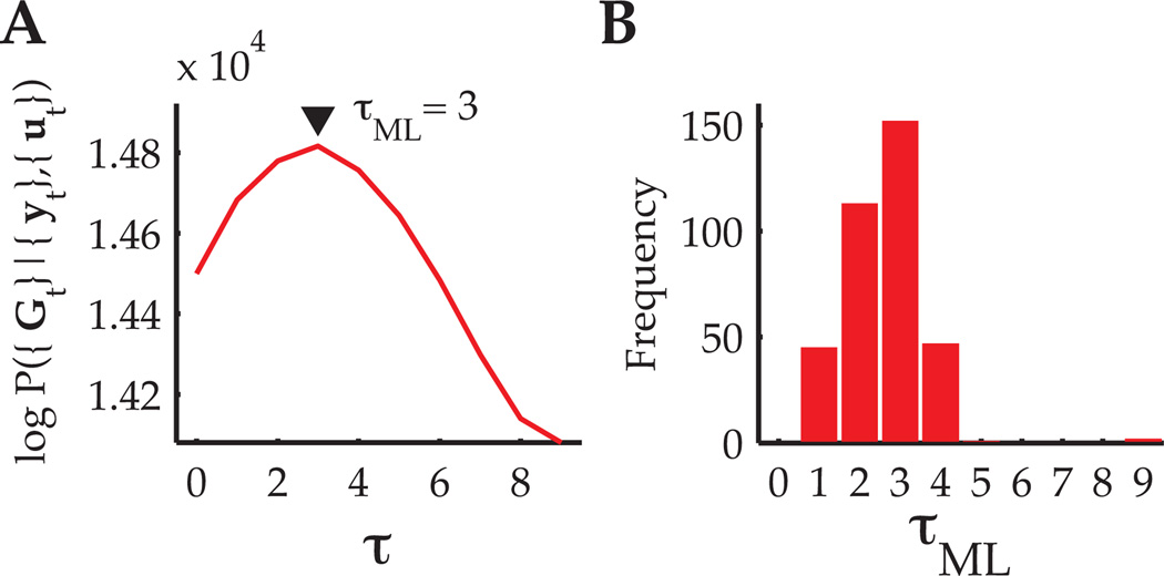
To determine the feedback delay, τ, we fit IME models for τ ∈ {0, …, 9} and assessed model fit by examining the data likelihood, P({G_t}|{y_t}, {u_t}). Recall that τ controls the number of latent variables, x, in each row of the graphical model in Fig. 1, and that the number of model parameters does not depend on the setting of τ. Fig. 4A shows the training data log-likelihood for a single BMI session across all evaluated choices of τ, and Fig. 4B gives the values of τ that maximized each training fold’s data log-likelihood. A feedback delay of 3 timesteps (100 ms) most often gave the best model fit. This result agrees with reaction times we measured from BMI cursor trajectories and previously reported motor-cortical latencies to visual stimuli (Schwartz et al., 1988).

Figure 4.

Model selection for determining the feedback delay, τ. (A) Log-likelihood as a function of τ over training data from a single BMI experiment. For this representative experiment, the feedback delay that maximized the data likelihood was τ_ML = 3 timesteps (100 ms). (B) Histogram of τ_ML values across 36 experiments (10 folds each).

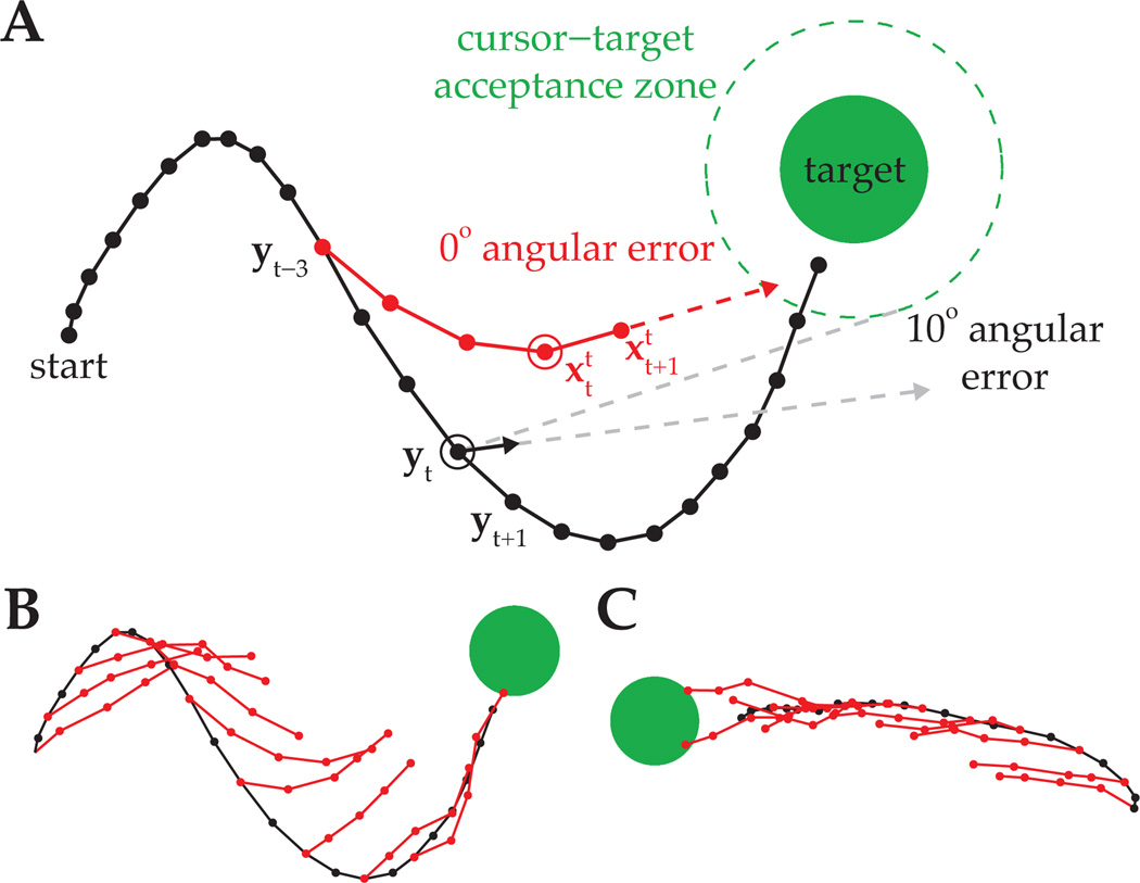
On many BMI trials, the subject drove the cursor roughly straight to the target, whereas cursor trajectories were more circuitous on other trials. It is an open question as to why the subject does not always drive the cursor straight to the target. In Figs. 5A and 5B, we show a BMI trial with a circuitous cursor trajectory, along with cross-validated IME-inferred internal estimates of cursor position from (13). In Fig. 5A, the subject’s aiming intention at timestep t, as defined by IME predictions of the subject’s internal state estimates ${\mathbf{x}}_{\mathrm{t}}^{\mathrm{t}}$ and ${\mathbf{x}}_{\mathrm{t}+1}^{\mathrm{t}}$, points straight toward the target. We would evaluate this aiming command as having a 0° angular error because the cursor would have hit the target had it continued along that intended aiming direction. For comparison, we computed velocity motor commands, v_t, through the actual cursor dynamics:

$${\mathbf{v}}_{\mathrm{t}}=\frac{1}{\mathrm{\Delta }t}(\mathit{\beta }{\mathbf{u}}_{\mathrm{t}}+{\beta }_0)$$ (14)

which correspond to the single-timestep (Δt = 33ms) contribution to the current cursor velocity, implicit in (8). In Fig. 5A, if the subject was aiming from a perfect prediction of the current cursor position, y_t, (e.g., by using an internal model that exactly matched the cursor dynamics), the motor command decoded from the actual cursor dynamics would miss the target by 10°.

Figure 5.

Evaluation of IME predictions. (A) Cursor trajectory (black line) from a BMI trial that was not used in model fitting. Red points are IME-inferred internal estimates of cursor position as determined by (13). Black arrow is the single-timestep velocity command, v_t, as computed through the actual cursor dynamics (14). Task success occurs when the cursor visibly overlaps with the target, which happens when the center of the cursor enters the cursor-target overlap zone (dashed green circle). (B) IME-inferred internal state chains across the entire BMI cursor trajectory from (A). (C) BMI cursor trajectory and IME-inferred internal state chains from a different trial.

Despite the cursor’s circuitous trajectory in this example trial, IME predictions suggest that the subject was indeed aiming straight toward the target throughout the trial (Fig. 5B). IME-extracted internal state estimates diverge from the true cursor trajectory because the extracted internal model differs from the true cursor dynamics (8). The key insights here are that i) the subject appears to be aiming from where it believes the cursor is at each point in time, as determined by the internal model, and ii) the subject’s neural commands, when evaluated through the internal model, are consistent with straight-to-target movements.

In Fig. 5C, we show a representative trial where the subject drove the BMI cursor along a more direct path to the target. On this trial and many similar to it, IME predictions of the subject’s internal state estimates tend to agree quite closely with the actual cursor movement. This agreement contrasts with the disagreement between IME predictions and cursor movements in Figs. 5A and 5B, highlighting the redundancy in the mapping from high-dimensional neural activity to low-dimensional cursor kinematics. Certain patterns of neural activity may produce straight-to-target movements through both the subject’s internal model and the cursor dynamics, whereas other patterns may produce straight-to-target movements through the internal model, but not through the cursor dynamics. On both trials in Fig. 5, IME-extracted internal models reveal the subject’s internal state estimates tending toward the target, regardless of where the actual cursor moves.

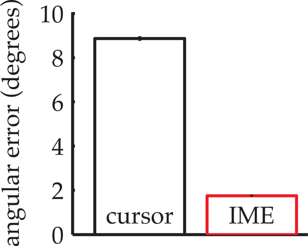
Across 5,760 trials from 36 BMI experiments, we computed cross-validated angular aiming errors from IME-inferred internal state estimates (as in the red angular error from Fig. 5A) and from actual cursor positions (as in the black angular error from Fig. 5A). IME-based aiming errors were about 5 times smaller than the analogous errors in demonstrated cursor trajectories (Fig. 6). Recall that the straight-to-target aiming assumption is only applied to the training data during model fitting and not when evaluating test data. That being said, neural commands in the test data were more consistent with straight-to-target aiming under IME-extracted internal models than under the actual cursor dynamics. Internal models extracted by IME therefore explain the subject’s neural commands better than the actual cursor dynamics.

Figure 6.

Angular aiming errors based on internal models estimated by IME (red bar) compared to errors based on internal models which exactly match the cursor dynamics (black bar). Angular errors were first averaged within each trial, then averaged across all 160 trials from each of 36 BMI experiments. Error bars indicate +/− SEM (n=5,760).

5. Discussion

The developed IME framework describes the internal state estimation process, whereby the subject integrates feedback with previously issued control signals to generate an up-to-date estimate of the plant state. IME specifically addresses complicating realities inherent in learning from demonstration, including i) sensory feedback delays and ii) mismatch between the true plant model and the subject’s internal model. This mismatch, often referred as model bias, is typically treated as an obstacle to be overcome, for example by incorporating model uncertainty in policy search (Deisenroth & Rasmussen, 2011) or through policy improvement in the presence of model inaccuracies (Abbeel et al., 2006). In this work, we seek to explicitly identify the subject’s internal model, rather than attempt to factor it out.

The internal model estimation problem that we address is fundamentally different from the problem of learning the actual plant dynamics (i.e., system identification). The internal model estimation problem cannot be solved by simply relating control signals to state transitions. Actual plant state trajectories only enter IME as delayed feedback, and as such, the actual plant dynamics play only an indirect role when extracting the subject’s internal model. Additionally, the objective in this work is not to design better plant dynamics, but rather to estimate the subject’s knowledge of the current plant dynamics, whatever they may be. The ability to extract the subject’s internal model depends critically on the consistency of control relative to the task goals and internal model, and not on the extent to which the subject’s demonstrations achieve those goals through the actual plant dynamics.

Ground truth cannot be known in the BMI application. For comparison against our IME-based results, we present aiming errors resulting from evaluating recorded neural commands through the true cursor dynamics. We chose this comparison because, for optimal control, the subject should learn an internal model that matches the actual plant dynamics. Although the subject is proficient in BMI tasks, our results suggest a mismatch between the subject’s internal model and the actual cursor dynamics. IME provides the opportunity to study the brain’s deviations from optimality, which may ultimately enable researchers to design specific training paradigms to improve a subject’s learning.

While IME requires specification of a cost function, we have demonstrated notable flexibility in this requirement. Unlike optimal control in the linear-quadratic Gaussian setting (Anderson & Moore, 1990), IME does not require pre-specification of a control time horizon. Additionally, by learning the c_t in (12), internal model estimation becomes agnostic to control effort. This feature is advantageous because the form of control costs is often unknown, especially in the BMI setting (although see (Körding & Wolpert, 2004)). In some cases, these control costs may be known a priori, and we are interested in extending IME to handle these scenarios (e.g., when a full quadratic cost function of state and control is specified).

One potential limitation of IME is the prescription of a static linear-Gaussian form to the internal model. Some applications may require more expressive internal model dynamics, which could be accommodated by a nonparametric representation of the internal model (Deisenroth et al., 2012). Additionally, the ability to extract a time-varying internal model may be needed in settings where the subject updates an internal model as control experience accrues.

APPENDIX

EM algorithm for the IME probabilistic framework described in Section 3:

Expectation Step

$$\begin{gathered} {\mathit{\mu }}_{\mathrm{t}-\tau }^{\mathrm{t}}=\mathbf{H}{\mathbf{y}}_{\mathrm{t}-\tau } \\ {\mathit{\mu }}_{\mathrm{k}+1}^{\mathrm{t}}=\mathbf{A}{\mathit{\mu }}_{\mathrm{k}}^{\mathrm{t}}+\mathbf{B}{\mathbf{u}}_{\mathrm{k}}+{\mathbf{b}}_0 \\ {\mathbf{\Sigma }}_{{\mathbf{x}}_{\mathrm{t}-\tau }^{\mathrm{t}},{\mathbf{x}}_{\mathrm{t}-\tau }^{\mathrm{t}}}={\mathbf{W}}_0 \\ {\mathbf{\Sigma }}_{{\mathbf{x}}_{\mathrm{k}+1}^{\mathrm{t}},{\mathbf{x}}_{\mathrm{k}+1}^{\mathrm{t}}}=\mathbf{A}{\mathbf{\Sigma }}_{{\mathbf{x}}_{\mathrm{k}}^{\mathrm{t}},{\mathbf{x}}_{\mathrm{k}}^{\mathrm{t}}}\mathbf{A}\prime +\mathbf{W} \\ {\mathbf{\Sigma }}_{{\mathbf{x}}_{\mathrm{k}}^{\mathrm{t}},{\mathbf{x}}_{\mathrm{k}+\mathrm{d}+1}^{\mathrm{t}}}={\mathbf{\Sigma }}_{{\mathbf{x}}_{\mathrm{k}}^{\mathrm{t}},{\mathbf{x}}_{\mathrm{k}+\mathrm{d}}^{\mathrm{t}}}\mathbf{A}\prime \end{gathered}$$

$$\begin{gathered} {\mathbf{\Sigma }}_{\mathbf{x}}=\left[\begin{array}{ccc}\hfill {\mathbf{\Sigma }}_{{\mathbf{x}}_{\mathrm{t}-\tau }^{\mathrm{t}},{\mathbf{x}}_{\mathrm{t}-\tau }^{\mathrm{t}}}\hfill & \hfill \dots \hfill & \hfill {\mathbf{\Sigma }}_{{\mathbf{x}}_{\mathrm{t}-\tau }^{\mathrm{t}},{\mathbf{x}}_{\mathrm{t}+1}^{\mathrm{t}}}\hfill \\ \hfill ⋮\hfill & \hfill \ddots \hfill & \hfill ⋮\hfill \\ \hfill {\mathbf{\Sigma }}_{{\mathbf{x}}_{\mathrm{t}+1}^{\mathrm{t}},{\mathbf{x}}_{\mathrm{t}-\tau }^{\mathrm{t}}}\hfill & \hfill \dots \hfill & \hfill {\mathbf{\Sigma }}_{{\mathbf{x}}_{\mathrm{t}+1}^{\mathrm{t}},{\mathbf{x}}_{\mathrm{t}+1}^{\mathrm{t}}}\hfill \end{array}\right] \\ {\mathit{\mu }}_{\mathrm{t}}=\left[\begin{array}{c}\hfill {\mathit{\mu }}_{\mathrm{t}-\tau }^{\mathrm{t}}\hfill \\ \hfill ⋮\hfill \\ \hfill {\mathit{\mu }}_{\mathrm{t}+1}^{\mathrm{t}}\hfill \end{array}\right] \end{gathered}$$

$$\begin{gathered} {\mathbf{\Gamma }}_{\mathrm{t}}={\mathbf{C}}_{\mathrm{t}}{\mathit{\mu }}_{\mathrm{t}+1}^{\mathrm{t}} \\ {\mathbf{\Sigma }}_{{\mathbf{G}}_{\mathrm{t}}}={\mathbf{C}}_{\mathrm{t}}{\mathbf{\Sigma }}_{{\mathbf{x}}_{\mathrm{t}+1}^{\mathrm{t}},{\mathbf{x}}_{\mathrm{t}+1}^{\mathrm{t}}}{\mathbf{C}}_{\mathrm{t}}\prime +\mathbf{V} \\ {\mathbf{\Sigma }}_{\mathbf{x},{\mathbf{G}}_{\mathrm{t}}}=\left[\begin{array}{c}\hfill {\mathbf{\Sigma }}_{{\mathbf{x}}_{\mathrm{t}-\tau }^{\mathrm{t}},{\mathbf{x}}_{\mathrm{t}+1}^{\mathrm{t}}}\hfill \\ \hfill ⋮\hfill \\ \hfill {\mathbf{\Sigma }}_{{\mathbf{x}}_{\mathrm{t}+1}^{\mathrm{t}},{\mathbf{x}}_{\mathrm{t}+1}^{\mathrm{t}}}\hfill \end{array}\right]{\mathbf{C}}_{\mathrm{t}}\prime \end{gathered}$$

$$\begin{gathered} {\mathit{\mu ̃}}_{\mathrm{t}}={\mathit{\mu }}_{\mathrm{t}}+{\mathbf{\Sigma }}_{\mathbf{x},{\mathbf{G}}_{\mathrm{t}}}{\mathbf{\Sigma }}_{{\mathbf{G}}_{\mathrm{t}}}^{-1}({\mathbf{G}}_{\mathrm{t}}-{\mathbf{\Gamma }}_{\mathrm{t}}) \\ {\mathbf{\Sigma ̃}}_{\mathbf{x}}={\mathbf{\Sigma }}_{\mathbf{x}}-{\mathbf{\Sigma }}_{\mathbf{x},{\mathbf{G}}_{\mathrm{t}}}{\mathbf{\Sigma }}_{{\mathbf{G}}_{\mathrm{t}}}^{-1}{\mathbf{\Sigma }}_{\mathbf{x},{\mathbf{G}}_{\mathrm{t}}}\prime \end{gathered}$$

Maximization Step

$$\begin{gathered} \mathbf{H}=(\sum _{t=1}^T{\mathit{\mu ̃}}_{\mathrm{t}-\tau }^{\mathrm{t}}({\mathbf{y}}_{\mathrm{t}-\tau })\prime ){(\sum _{t=1}^T{\mathbf{y}}_{\mathrm{t}-\tau }({\mathbf{y}}_{\mathrm{t}-\tau })\prime )}^{-1} \\ {\mathbf{W}}_0=\frac{1}{T}\sum _{t=1}^T({\mathbf{\Sigma ̃}}_{{\mathbf{x}}_{\mathrm{t}-\tau }^{\mathrm{t}},{\mathbf{x}}_{\mathrm{t}-\tau }^{\mathrm{t}}}+{\mathit{\mu ̃}}_{\mathrm{t}-\tau }^{\mathrm{t}}({\mathit{\mu ̃}}_{\mathrm{t}-\tau }^{\mathrm{t}})\prime -\mathbf{H}{\mathbf{y}}_{\mathrm{t}-\tau }({\mathit{\mu ̃}}_{\mathrm{t}-\tau }^{\mathrm{t}})\prime ) \\ {\mathbf{P}}_{\mathrm{k}}^{\mathrm{t}}=[{\mathbf{\Sigma ̃}}_{{\mathbf{x}}_{\mathrm{k}+1}^{\mathrm{t}},{\mathbf{x}}_{\mathrm{k}}^{\mathrm{t}}}+{\mathit{\mu ̃}}_{\mathrm{k}+1}^{\mathrm{t}}({\mathit{\mu ̃}}_{\mathrm{k}}^{\mathrm{t}})\prime {\mathit{\mu ̃}}_{\mathrm{k}+1}^{\mathrm{t}}{\mathbf{u}}_{\mathrm{k}}\prime {\mathit{\mu ̃}}_{\mathrm{k}+1}^{\mathrm{t}}] \\ {\mathbf{Q}}_{\mathrm{k}}^{\mathrm{t}}=\left[\begin{array}{ccc}\hfill {\mathbf{\Sigma ̃}}_{{\mathbf{x}}_{\mathrm{k}}^{\mathrm{t}},{\mathbf{x}}_{\mathrm{k}}^{\mathrm{t}}}+{\mathit{\mu ̃}}_{\mathrm{k}}^{\mathrm{t}}({\mathit{\mu ̃}}_{\mathrm{k}}^{\mathrm{t}})\prime \hfill & \hfill {\mathit{\mu ̃}}_{\mathrm{k}+1}^{\mathrm{t}}{\mathbf{u}}_{\mathrm{k}}\prime \hfill & \hfill {\mathit{\mu ̃}}_{\mathrm{k}}^{\mathrm{t}}\hfill \\ \hfill {\mathbf{u}}_{\mathrm{k}}({\mathit{\mu ̃}}_{\mathrm{k}}^{\mathrm{t}})\prime \hfill & \hfill {\mathbf{u}}_{\mathrm{k}}{\mathbf{u}}_{\mathrm{k}}\prime \hfill & \hfill {\mathbf{u}}_{\mathrm{k}}\hfill \\ \hfill ({\mathit{\mu ̃}}_{\mathrm{k}}^{\mathrm{t}})\prime \hfill & \hfill {\mathbf{u}}_{\mathrm{k}}\prime \hfill & \hfill 1\hfill \end{array}\right] \\ \mathbf{M}=[\mathbf{A}\mathbf{B}{\mathbf{b}}_0]=\left(\sum _{t=1}^T\sum _{k=t-\tau }^T{\mathbf{P}}_{\mathrm{k}}^{\mathrm{t}}\right){\left(\sum _{t=1}^T\sum _{k=t-\tau }^T{\mathbf{Q}}_{\mathrm{k}}^{\mathrm{t}}\right)}^{-1} \\ \mathbf{W}=\frac{1}{\tau \times T}\sum _{t=1}^T\sum _{k=t-\tau }^T({\mathbf{\Sigma ̃}}_{{\mathbf{x}}_{\mathrm{k}}^{\mathrm{t}},{\mathbf{x}}_{\mathrm{k}}^{\mathrm{t}}}+{\mathit{\mu ̃}}_{\mathrm{k}}^{\mathrm{t}}({\mathit{\mu ̃}}_{\mathrm{k}}^{\mathrm{t}})\prime -\mathbf{M}{\mathbf{P}}_{\mathrm{k}}^{\mathrm{t}}\prime ) \\ \mathbf{C}=(\sum _{t=1}^T{\mathbf{G}}_{\mathrm{t}}({\mathit{\mu ̃}}_{\mathrm{t}+1}^{\mathrm{t}})\prime ){(\sum _{t=1}^T{\mathbf{\Sigma ̃}}_{{\mathbf{x}}_{\mathrm{k}+1}^{\mathrm{t}},{\mathbf{x}}_{\mathrm{k}+1}^{\mathrm{t}}}+{\mathit{\mu ̃}}_{\mathrm{t}+1}^{\mathrm{t}}({\mathit{\mu ̃}}_{\mathrm{t}+1}^{\mathrm{t}})\prime )}^{-1} \\ \mathbf{V}=\frac{1}{T}\sum _{t=1}^T({\mathbf{G}}_{\mathrm{t}}{\mathbf{G}}_{\mathrm{t}}\prime -{\mathbf{C}}_{\mathrm{t}}{\mathit{\mu ̃}}_{\mathrm{t}+1}^{\mathrm{t}}{\mathbf{G}}_{\mathrm{t}}\prime ) \end{gathered}$$

For the IME variant from Section 4, update the above Estep with the following:

$$\begin{gathered} \mathbf{H}=\mathbf{I} \\ {\mathbf{W}}_0=\mathbf{0} \\ \mathbf{W}={\sigma }_{\mathbf{x}}^2\mathbf{I} \\ \mathbf{V}={\sigma }_{\mathbf{G}}^2\mathbf{I} \\ {\mathbf{C}}_{\mathrm{t}}=[(1+{\mathrm{c}}_{\mathrm{t}})\mathbf{I}-{\mathrm{c}}_{\mathrm{t}}\mathbf{I}] \\ {\mathbf{\Gamma }}_{\mathrm{t}}={\mathbf{C}}_{\mathrm{t}}\left[\begin{array}{c}\hfill {\mathit{\mu }}_{\mathrm{t}+1}^{\mathrm{t}}\hfill \\ \hfill {\mathit{\mu }}_{\mathrm{t}}^{\mathrm{t}}\hfill \end{array}\right] \\ {\mathbf{\Sigma }}_{{\mathbf{G}}_{\mathrm{t}}}={\mathbf{C}}_{\mathrm{t}}\left[\begin{array}{cc}\hfill {\mathbf{\Sigma }}_{{\mathbf{x}}_{\mathrm{t}+1}^{\mathrm{t}},{\mathbf{x}}_{\mathrm{t}+1}^{\mathrm{t}}}\hfill & \hfill {\mathbf{\Sigma }}_{{\mathbf{x}}_{\mathrm{t}+1}^{\mathrm{t}},{\mathbf{x}}_{\mathrm{t}}^{\mathrm{t}}}\hfill \\ \hfill {\mathbf{\Sigma }}_{{\mathbf{x}}_{\mathrm{t}}^{\mathrm{t}},{\mathbf{x}}_{\mathrm{t}+1}^{\mathrm{t}}}\hfill & \hfill {\mathbf{\Sigma }}_{{\mathbf{x}}_{\mathrm{t}}^{\mathrm{t}},{\mathbf{x}}_{\mathrm{t}}^{\mathrm{t}}}\hfill \end{array}\right]{\mathbf{C}}_{\mathrm{t}}\prime +\mathbf{V} \\ {\mathbf{\Sigma }}_{\mathbf{x},{\mathbf{G}}_{\mathrm{t}}}=\left[\begin{array}{cc}\hfill {\mathbf{\Sigma }}_{{\mathbf{x}}_{\mathrm{t}-\tau }^{\mathrm{t}},{\mathbf{x}}_{\mathrm{t}+1}^{\mathrm{t}}}\hfill & \hfill {\mathbf{\Sigma }}_{{\mathbf{x}}_{\mathrm{t}-\tau }^{\mathrm{t}},{\mathbf{x}}_{\mathrm{t}}^{\mathrm{t}}}\hfill \\ \hfill ⋮\hfill & \hfill ⋮\hfill \\ \hfill {\mathbf{\Sigma }}_{{\mathbf{x}}_{\mathrm{t}+1}^{\mathrm{t}},{\mathbf{x}}_{\mathrm{t}+1}^{\mathrm{t}}}\hfill & \hfill {\mathbf{\Sigma }}_{{\mathbf{x}}_{\mathrm{t}+1}^{\mathrm{t}},{\mathbf{x}}_{\mathrm{t}}^{\mathrm{t}}}\hfill \end{array}\right]{\mathbf{C}}_{\mathrm{t}}\prime \end{gathered}$$

and in the M-step, take:

$$\begin{gathered} {\sigma }_{\mathbf{x}}^2=\frac{1}{2}tr(\mathbf{W}){\sigma }_{\mathbf{G}}^2=\frac{1}{2}tr(\mathbf{V}) \\ {\alpha }_{1,\mathrm{t}}=({\mathit{\mu ̃}}_{\mathrm{t}+1}^{\mathrm{t}}-{\mathit{\mu ̃}}_{\mathrm{t}}^{\mathrm{t}})({\mathbf{G}}_{\mathrm{t}}-{\mathit{\mu ̃}}_{\mathrm{t}+1}^{\mathrm{t}})\prime +{\mathbf{\Sigma ̃}}_{{\mathbf{x}}_{\mathrm{t}}^{\mathrm{t}},{\mathbf{x}}_{\mathrm{t}+1}^{\mathrm{t}}}-{\mathbf{\Sigma ̃}}_{{\mathbf{x}}_{\mathrm{t}+1}^{\mathrm{t}},{\mathbf{x}}_{\mathrm{t}+1}^{\mathrm{t}}} \\ {\alpha }_{2,\mathrm{t}}=({\mathit{\mu ̃}}_{\mathrm{t}+1}^{\mathrm{t}}-{\mathit{\mu ̃}}_{\mathrm{t}}^{\mathrm{t}})({\mathit{\mu ̃}}_{\mathrm{t}+1}^{\mathrm{t}}-{\mathit{\mu ̃}}_{\mathrm{t}}^{\mathrm{t}})\prime +{\mathbf{\Sigma ̃}}_{{\mathbf{x}}_{\mathrm{t}+1}^{\mathrm{t}},{\mathbf{x}}_{\mathrm{t}+1}^{\mathrm{t}}}+{\mathbf{\Sigma ̃}}_{{\mathbf{x}}_{\mathrm{t}}^{\mathrm{t}},{\mathbf{x}}_{\mathrm{t}}^{\mathrm{t}}}-2{\mathbf{\Sigma ̃}}_{{\mathbf{x}}_{\mathrm{t}+1}^{\mathrm{t}},{\mathbf{x}}_{\mathrm{t}}^{\mathrm{t}}} \\ {\mathrm{c}}_{\mathrm{t}}=\text{max}(0,\frac{tr({\alpha }_{1,\mathrm{t}})}{tr({\alpha }_{2,\mathrm{t}})}) \end{gathered}$$

References

- Abbeel P, Ng AY. Apprenticeship learning via inverse reinforcement learning; Proc. 21st International Conf. on Machine Learning; 2004. pp. 1–8. [Google Scholar]
- Abbeel P, Quigley M, Ng AY. Using inaccurate models in reinforcement learning; Proc. 23rd International Conf. on Machine learning; 2006. pp. 1–8. [Google Scholar]
- Anderson BDO, Moore JB. Optimal control: linear quadratic methods. Upper Saddle River, NJ, USA: Prentice-Hall, Inc; 1990. [Google Scholar]
- Boyd S, El Ghaoui L, Feron E, Balakrishnan V. Studies in Applied Mathematics. Philadelphia, PA: 1994. Linear Matrix Inequalities in System and Control Theory. [Google Scholar]
- Chase SM, Kass RE, Schwartz AB. Behavioral and neural correlates of visuomotor adaptation observed through a brain-computer interface in primary motor cortex. J. Neurophysiol. 2012;108(2):624–644. doi: 10.1152/jn.00371.2011. [DOI] [PMC free article] [PubMed] [Google Scholar]
- Coates A, Abbeel P, Y Ng AY. Learning for control from multiple demonstrations; Proc. 25th International Conf. on Machine Learning; 2008. pp. 144–151. [Google Scholar]
- Crapse TB, Sommer MA. Corollary discharge across the animal kingdom. Nat. Rev. Neurosci. 2008;9(8):587–600. doi: 10.1038/nrn2457. [DOI] [PMC free article] [PubMed] [Google Scholar]
- Deisenroth MP, Rasmussen CE. Pilco: A model-based and data-efficient approach to policy search; Proc. 28th International Conf. on Machine Learning; 2011. pp. 465–472. [Google Scholar]
- Deisenroth MP, Turner RD, Huber MF, Hanebeck UD, Rasmussen CE. Robust filtering and smoothing with gaussian processes. IEEE Trans. Automatic Control. 2012;57(7):1865–1871. [Google Scholar]
- Dempster AP, Laird NM, Rubin DB. Maximum likelihood from incomplete data via the EM algorithm. J. Royal Stat. Soc., Series B. 1977;39(1):1–38. [Google Scholar]
- Ganguly K, Dimitrov DF, Wallis JD, Carmena JM. Reversible large-scale modification of cortical networks during neuroprosthetic control. Nature Neurosci. 2011;14(5):662–667. doi: 10.1038/nn.2797. [DOI] [PMC free article] [PubMed] [Google Scholar]
- Georgopoulos AP, Caminiti R, Kalaska JF, Massey JT. Spatial coding of movement: a hypothesis concerning the coding of movement direction by motor cortical populations. Exp. Brain Res. Suppl. 1983;7:327–336. [Google Scholar]
- Green AM, Kalaska JF. Learning to move machines with the mind. Trends Neurosci. 2011;34(2):61–75. doi: 10.1016/j.tins.2010.11.003. [DOI] [PubMed] [Google Scholar]
- Körding KP, Wolpert DM. The loss function of sensorimotor learning. Proc. Natl. Acad. Sci. 2004;101(26):9839–9842. doi: 10.1073/pnas.0308394101. [DOI] [PMC free article] [PubMed] [Google Scholar]
- Miall RC, Wolpert DM. Forward models for physiological motor control. Neural Networks. 1996;9(8):1265–1279. doi: 10.1016/s0893-6080(96)00035-4. [DOI] [PubMed] [Google Scholar]
- Ng AY, Russell S. Algorithms for inverse reinforcement learning; Proc. 17th International Conf. on Machine Learning; 2000. pp. 663–670. [Google Scholar]
- Ratliff ND, Bagnell JA, Zinkevich Martin. Maximum margin planning; Proc. 23rd International Conf. on Machine Learning; 2006. pp. 729–736. [Google Scholar]
- Schaal S. Is imitation learning the route to humanoid robots? Trends in Cognitive Sciences. 1999;3(6):233–242. doi: 10.1016/s1364-6613(99)01327-3. [DOI] [PubMed] [Google Scholar]
- Schwartz AB, Kettner RE, Georgopoulos AP. Primate motor cortex and free arm movements to visual targets in 3-dimensional space. 1. relations between single cell discharge and direction of movement. J. Neurosci. 1988;8(8):2913–2927. doi: 10.1523/JNEUROSCI.08-08-02913.1988. [DOI] [PMC free article] [PubMed] [Google Scholar]
- Taylor DM, Helms Tillery SI, Schwartz AB. Direct cortical control of 3D neuroprosthetic devices. Science. 2002;296:1829–1832. doi: 10.1126/science.1070291. [DOI] [PubMed] [Google Scholar]
- Ziebart BD, Maas AL, Bagnell JA, Dey AK. Maximum entropy inverse reinforcement learning; Proc. 23rd AAAI Conf. on Artificial Intelligence; 2008. pp. 1433–1438. [Google Scholar]