Identifying Genetic Interactions in Genome-Wide Data Using Bayesian Networks

Abstract

It is believed that interactions among genes (epistasis) may play an important role in susceptibility to common diseases [Moore and Williams, 2002; Ritchie et al., 2001].

To study the underlying genetic variants of diseases, genome-wide association studies (GWAS) that simultaneously assay several hundreds of thousands of SNPs are being increasingly used. Often, the data from these studies are analyzed with single-locus methods [Lambert et al., 2009; Reiman et al., 2007]. However, epistatic interactions may not be easily detected with single-locus methods [Marchini et al., 2005]. As a result, both parametric and nonparametric multi-locus methods have been developed to detect such interactions [Heidema et al., 2006]. However, efficiently analyzing epistasis using high-dimensional genome-wide data remains a crucial challenge.

We develop a method based on Bayesian networks and the minimum description length principle for detecting epistatic interactions. We compare its ability to detect gene-gene interactions and its efficiency to that of the combinatorial method multifactor dimensionality reduction (MDR) using 28000 simulated data sets generated from 70 different genetic models We further apply the method to over 300,000 SNPs obtained from a GWAS involving late onset Alzheimer’s disease (LOAD). Our method outperforms MDR and we substantiate previous results indicating that the GAB2 gene is associated with LOAD. To our knowledge, this is the first successful model-based epistatic analysis using a high-dimensional genome-wide data set.

1 Introduction

Common diseases, like hypertension and Alzheimer’s disease, are believed to be multifactorial in origin being caused by genetic variants at multiple loci, with each locus conferring modest risk of developing the disease [Moore and Williams, 2002]. In addition, interactions among genetic variants at multiple loci and between genetic variants and environmental factors likely play a role in such diseases [Ritchie et al., 2001, Thornton-Wells et al., 2004; Nagel, 2005]. Multiple and complex interactions underlie gene expression and its regulation and there is evidence that gene-gene interactions and gene-environment interactions play a role in the determination of the phenotypes in common diseases [Kardia, 2000; Templeton, 2000]. Furthermore, [Smith and Lusis, 2002] argue that the majority of the socioeconomic burden of disease in industrialized nations is due to complex disorders, in which multiple genes interact with the environment to produce diseases. Examples include atherosclerosis, diabetes, cancer, multiple sclerosis, autism, alcoholism, and drug abuse [Diabetes Genetics Initiative et al., 2007; Easton et al., 2007; Moffatt et al., 2007; Samani et al., 2007; Scott et al., 2007; Steinthorsdottir et al., 2007; Wellcome Trust Case Control Consortium, 2007].

The most common type of genetic variation is the single nucleotide polymorphism (SNP) that results when a single nucleotide is replaced by another in the genome sequence. The development of high-throughput genotyping technologies that simultaneously assay many thousands of SNPs have led to a flurry of genome-wide association studies (GWAS) with the aim of discovering SNPs that either singly or in combination are associated with disease. Often, the data from such studies are analyzed with single-locus methods [Coon et al., 2007; Herbert et al., 2006; Lambert et al., 2009; Reiman et al., 2007]. Loci that interact in complex ways may not be easily detected with such methods [Marchini et al., 2005].

One important example of gene-gene interaction is epistasis. Biologically, epistasis refers to gene-gene interaction when the action of one gene is modified by one or several other genes. Statistically, epistasis refers to interaction between genetic variants at multiple loci in which the net effect on disease from the combination of genotypes at the different loci is not accurately predicted by a simple linear combination of the individual genotype effects. The detection of statistical epistasis has the potential to identify interacting genetic loci that may underlie the inheritance of common diseases.

It is difficult to detect epistatic relationships statistically due to the sparseness of the data and the non-linearity of the relationships [Velez et al., 2007]. New statistical and computational methods have recently been developed to identify and characterize epistatic interactions. Parametric methods include logistic regression [Millstein et al., 2005] and non-parametric methods based on machine-learning include combinatorial methods, set association analysis, genetic programming, neural networks and random forests. These latter methods have been summarized in a recent review [Heidema et al., 2006].

Combinatorial methods search over all possible combinations of loci to find combinations that are predictive of the phenotype. The combinatorial method multifactor dimensionality reduction (MDR) [Ritchie et al., 2001, Hahn et al., 2003; Velez et al., 2007] was designed to detect associations between multiple genetic markers and a phenotype by examining higher order interactions among SNPs in a case-control setting. MDR combines two or more variables into a single variable (hence leading to dimensionality reduction); this changes the representation space of the data and facilitates the detection of nonlinear interactions among the variables.

An advantage of MDR over traditional statistical modeling techniques like logistic regression lies in that MDR is a model-free method that does not require the specification of a genetic model. MDR has been successfully applied to detecting epistatic interactions in complex human diseases such as sporadic breast cancer, cardiovascular disease, and type II diabetes in genomic data containing less than 30 SNPs [Richie et al., 2001, Coffey et al., 2004, Cho et al., 2004].

A crucial challenge is the development of methods that can efficiently identify epistasis in genome-wide data sets that typically contains hundreds of thousands of SNPs. To use a combinatorial method to examine all possible subsets containing even a small number of SNPs is intractable. For example, investigation of all possible subsets containing five SNPs, in a genome wide data set that has 500,000 SNPs, would require examining 2.6041×10²⁶ subsets, an astronomically large number.

In this paper, we develop and evaluate a multi-locus method for detecting genetic interactions based on Bayesian networks and the minimum description length principle. We compare its ability to detect epistatic interactions and its computational efficiency to that of MDR using 28,000 simulated data sets generated from 70 different genetic models [Velez et al., 2007]. Furthermore, we apply the method to a late onset Alzheimer’s disease (LOAD) GWAS data set that contains over 300,000 SNPs. It is well-known that the apoplipoprotein E (APOE) gene is associated with LOAD [Coon et al., 2007; Papassotiropoulos et al., 2006; Corder et al., 1993]. The APOE gene has three common variants ε2, ε3, and ε4. The least risk is associated with the ε2 allele, while each copy of the ε4 allele increases the risk. We substantiate previous results indicating that the GAB2 gene modifies LOAD susceptibility in APOE ε4 carriers. To our knowledge, this is the first successful model-based epistatic analysis of a high-dimensional genome-wide data set. A strength of our method is that we should be able to extend it using a heuristic search, thereby making it capable of investigating complex gene-gene interactions in a genome-wide data.

2 Method

We now describe our new method for detecting gene-gene interactions which we call the Bayesian network minimum bit length (BNMBL) method. We first briefly introduce Bayesian networks; then we give details of the BNMBL method.

2.1 Bayesian Networks

A Bayesian network (BN) [Jensen and Nielsen, 2007; Neapolitan, 2004] is a probabilistic model that consists of a directed acyclic graph (DAG) G = (V,E), where V is the set of vertices in G and E is the set of edges, such that (G,P) satisfy the Markov Condition. (GP,) satisfies the Markov condition if for each variable X ∈ V, X is conditionally independent of the set of all its nondescendents given the set of all its parents. It is possible to prove that (G,P) satisfies the Markov condition if and only if P is equal to the product of its conditional distributions of all nodes given their parents in G, whenever these conditional distributions exist [Neapolitan, 2004]. That is, if our variables are X₁, X₂,…, X_n, and PA_i is the set of parents of X_i, then

$$P(X_1,X_2,\dots ,X_n)=\prod _{i=1}^{n}P(X_i\mid {PA}_i).$$

So a BN is ordinarily represented by the DAG G and the conditional probability distributions, which are called the parameters in the BN. Using a BN inference algorithm [Jensen and Nielsen, 2007; Neapolitan, 2004], we can determine conditional probabilities of nodes of interest in a BN given other nodes have certain values.

Methods for learning both the structure and parameters in BNs from data have been developed [Neapolitan, 2004]. A well-known method for learning a BN from data searches over a space of BNs and selects the one that scores the highest on a Bayesian score [Cooper and Herskovits, 1992]. Due to compelling results in [Heckerman et al., 1995], when using the Bayesian score we need to assess the value of a hyper-parameter parameter α called the prior equivalent sample size. A dilemma when using the Bayesian score concerns the choice of α. Although various researchers have forwarded different choices based on philosophical/intuitive grounds [Neapolitan, 2004], no choice is commonly accepted. Moreover, [Silander et al., 2007] provide a number of examples of learning models from various data sets showing that the choice of α can greatly affect the selected model.

An alternative to the Bayesian score is an information-theoretic score that is based on the Minimum Description Length (MDL) principle [Rissanen, 1978]. According to this principle, the best model is one that minimizes the sum of the encoding lengths of the data and the model itself. To apply this principle to BNs, we must determine the number of bits needed to encode a BN model and the number of bits needed to encode the data given the BN model. [Suzuki, 1999] developed an MDL score for a BN as follows:

$$\sum _{i=1}^n\frac{d_i}{2}{log}_{2}m-m\sum _{i=1}^n\sum _{j=1}^{q_i}\sum _{k=1}^{r_i}P(x_{ik},{pa}_{ij}){log}_2\frac{P(x_{ik},{pa}_{ij})}{P(x_{ik})P({pa}_{ij})}.$$ (1)

The variable m is the number of data items, d_i is the number of parameters for the probability distribution for the i th node, r_i is the number of states of X_i, x_ik is the k th state of X_i, q_i is the number of instantiations of the parents of X_i, pa_ij is the j th instantiation of the parents of X_i, and the probabilities are computed using the data. The first term gives the number of bits required to encode the BN model and the second term gives the number of bits needed to encode the data given the model.

Typically the space of BN models for domains containing more than a few tens of variables is forbiddingly large. Thus, heuristic algorithms are used to search over the space of BN models [Neapolitan, 2004].

2.2 The BNMBL Method

We use BNs to model the association of genetic variants with a phenotype. In this application, a BN contains k parent nodes and a single child node, where the parent nodes are SNPs or other types of genetic variants and the child node is the phenotype or the disease of interest. Figure 1 shows such a model, which we call an epistatic DAG model (EpiDAG). The BNMBL method scores all such k-parent models up to a user-specified limit on k using an MDL-based score which we develop next.

Figure 1.

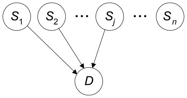
A 3-SNP EpiDAG. The total number of SNPs in the domain is n.

We need only score EpiDAGs like the one shown in Figure 1. Each parameter in a DAG model learned from data is a fraction with precision 1/m, where m is the number of data items. So it takes log₂ m bits to store each parameter. However, as explained in [Friedman, 1996], the higher order bits are not very useful, and we need use only $\frac{1}{2}{log}_{2}m$ bits to store a parameter. In this way we arrive at the DAG penalty in Equation 1 ([Suzuki, 1999] obtained the result in a different manner). Suppose that k SNPs have edges to D in one of our EpiDAG models. Since each SNP has three possible values there are 3^k instantiations of the parents of D. The average number of data items taking the value of each instantiation is m/3^k. If we approximate the precision for each of D’s parameters by this average, our penalty for each of these parameters is $\frac{1}{2}{log}_2\frac{m}{3^k}$. Since our penalty for each parameter in a parent SNP is $\frac{1}{2}{log}_{2}m$, our total DAG penalty for a given model is $\frac{3^k}{2}{log}_2\frac{m}{3^k}+\frac{2k}{2}{log}_{2}m$. When using this DAG penalty in Equation 1, we call the score the BNMBL score.

While MDR evaluates a k-SNP model using multifold cross-validation, BNMBL evaluates a k-SNP model directly using the BNMBL score without performing cross-validation, thereby making it more efficient.

$$\sum _{i=1}^n(\frac{3^k}{2}{log}_2\frac{m}{3^k}+\frac{2k}{2}{log}_{2}m)-m\sum _{i=1}^n\sum _{j=1}^{q_i}\sum _{k=1}^{r_i}P(x_{ik},{pa}_{ij}){log}_2\frac{P(x_{ik},{pa}_{ij})}{P(x_{ik})P({pa}_{ij})}.$$

3 Experiments

We performed experiments comparing the performance of BNMBL to that of MDR using synthetic data that was originally used to evaluate MDR, and we further evaluated BNMBL using a LOAD GWAS data set. MDR v. 1.25, which is available at www.epistasis.org, was used to run MDR. We implemented BNMBL in the Java programming language. All experiments were run on a PC running Windows XP with a 2.8 GHz processor and 3 GB of RAM.

3.1 Data sets

3.1.1 The Synthetic Data set

Our experiments used synthetic data based on 70 genetic models of epistatic interactions. Each model contains a different penetrance function that defines a probabilistic relationship between genotype and phenotype where susceptibility to disease depends on two interacting loci. The models, which are described in Supplementary Table 1 to [Velez et al., 2007], are distributed uniformly among seven broad-sense heritabilities ranging from 0.01 to 0.40 (0.01, 0.025, 0.05, 0.10, 0.20, 0.30, and 0.40) and two minor allele frequencies (0.2 and 0.4). To study the effect of sample size, from a given model, 100 data sets were generated for each of four sample sizes (200, 400, 800 and 1600) where each data set contains equal number of disease and healthy samples. For a generated pair of epistatic SNP values, a set of 18 SNPs that were assigned random values was appended to simulate SNPs that are non-informative with respect to the disease status. The data sets were obtained from http://discovery.dartmouth.edu/epistatic_data/VelezData.zip.

3.1.2 The GWAS Data set

The LOAD GWAS dataset contains the data from three cohorts and was originally analyzed in [Reiman et al., 2007]. Each record in this data set consists of genotype information, APOE status, and LOAD status for 1411 subjects. Of the 1411 subjects, 861 have LOAD and 550 do not, and 644 are APOE ε4 carriers and 767 are non-carriers. The study investigators typed 502,627 SNPs for each subject and after applying quality controls analyzed 312,316 SNPs.

The BNMBL method was applied to EpiDAGs in which the disease node (LOAD) has precisely two parents, one being the APOE gene and the other being one of the 312,316 SNPs. These models were scored using the LOAD data set mentioned above.

3.2 Evaluation Methodology

Using the synthetic data, the performances of MDR and BNMBL were compared on power (accuracy) and computational efficiency (speed). For a set of 100 data sets generated from a model, power refers to the number of data sets on which an algorithm correctly selects the model containing both interacting SNPs. The Wilcoxon two-sample paired signed rank test was used to compare the power of MDR and BNMBL.

[Subramanian et al., 2005] developed an enrichment score that represents the degree to which a set is overrepresented at the extreme top or bottom of an ordered list. This score was used to evaluate the results obtained from applying BNMBL to the GWAS data set.

3.3 Results

3.3.1 Results for the Synthetic Data Sets

Valez et al., 2007 showed that MDR had the lowest detection sensitivity for models 55–59 in Supplementary Table 1 to [Velez et al., 2007]. These models have the weakest broad-sense heritability (0.01) and a minor allele frequency of 0.2. Table 1 shows the powers for MDR and BNMBL for these 5 models. BNMBL outperformed MDR in 16 of the experiments involving the most difficult models, whereas MDR outperformed BNMBL only 2 times.

Table 1.

Columns MDR and BNMBL show the powers for each of the methods for models 55–59. “Total” is the sum of the powers over the five models.

Data set Size	Model	MDR	BNMBL
200	55	3	7
	56	3	4
	57	3	5
	58	3	7
	59	3	3
	Total (200)	15	26
400	55	8	8
	56	7	9
	57	11	9
	58	15	27
	59	8	7
	Total (400)	49	60
800	55	26	30
	56	22	36
	57	25	29
	58	49	67
	59	18	24
	Total (800)	140	186
1600	55	66	81
	56	59	83
	57	68	81
	58	88	96
	59	49	63
	Total (1600)	330	404

Table 2 shows the sums of the powers overall all 70 models and the p-values obtained from the Wilcoxon two-sample paired signed rank test comparing the powers of MDR and BNMBL over all 70 models. BNMBL significantly out-performed MDR on all sample sizes.

Table 2.

The sums of the powers over all 70 data sets for MDR and BNMBL appear in Columns 2 and 3, and p-values appear in Column 4.

n	MDR	BNMBL	p-value
200	4904	5016	0.009
400	5796	5909	0.004
800	6408	6517	0.003
1600	6792	6883	0.012

Table 1 shows that at large sample sizes (1600 data items), BNMBL correctly identified 74 more difficult models than MDR, while Table 2 indicates that at large sample sizes BNMBL correctly identified 91 more total models than MDR. The majority of the improvement obtained by using BNMBL concerns the difficult models.

Table 3 shows the mean running times in seconds obtained by averaging the running times over the data sets generated from all 70 genetic models. MDR is several orders of magnitude slower than BNMBL. The superior running time of BNMBL is due largely to its ability to use the entire data set for computing the score of each model, while MDR performs multi-fold cross-validation to score the models.

Table 3.

Mean running times in seconds.

n	MDR	BNMBL
200	119.81	0.0198
400	146.64	0.0307
800	207.98	0.0498
1600	241.74	0.0966

3.3.2 Results for the GWAS Data Set

We applied the BNMBL method to score EpiDAG models in which the disease node (LOAD) has precisely two parents, one being the APOE gene and the other being one of the 312,316 SNPs investigated. Each model was evaluated in the following three modes: 1) the model was scored after the heterozygote state of the SNP was grouped with the homozygote state containing the lower frequency allele; 2) the model was scored after the heterozygote state of the SNP was grouped with the homozygote state containing the higher frequency allele; and 3) the maximum of the scores obtained from 1 and 2 above was assigned to the model.

We briefly describe the results obtained by [Reiman et al., 2007] who investigated the association of these SNPs separately in APOEε4 carriers and in APOEε4 non-carriers. A discovery cohort and two replication cohorts were used in the study. Within the discovery subgroup consisting of APOEε 4 carriers, 10 of the 25 SNPs exhibiting the greatest association with LOAD (contingency test p-value 9×10⁻⁸ to 1×10⁻⁷) were located in the GRB-associated binding protein 2 (GAB2) gene on chromosome 11q14.1. Associations with LOAD for 6 of these SNPs were confirmed in the two replication cohorts. Combined data from all three cohorts exhibited significant association between LOAD and all 10 GAB2 SNPs. These 10 SNPs were not significantly associated with LOAD in the APOEε4 non-carriers.

[Reiman et al., 2007] used Haploview v3.32 to determine the linkage disequilibrium (LD) structure of the chromosome 11q14.1 region surrounding GAB2 in each of the three cohorts they investigated. The GAB2 gene is encompassed by a block extending from SNP rs901104 to SNP rs2373115. There are 18 GAB2 SNPs located on this block which survived Haploview’s quality metrics and were part of the significant haplotype. The investigators found that these 18 SNPs have three haplotypes, one extremely common one is associated with an increased risk for LOAD in APOE ε4 carriers, a second common one is associated with a decreased risk for LOAD in APOE ε4 carriers, and a third rare one is unrelated to LOAD in APOE ε4 carriers.

The SNPs we investigated contained 14 of these 18 SNPs. Table 4 shows their ranks among all 312,316 SNPs according to their BNMBL scores using Mode 1. Based on the enrichment score developed by [Subramanian et al., 2005] these 14 SNPs are significantly overrepresented near the top of the list of all SNPs (p-value = 3.9759 × 10 ^{− 47}).

Table 4.

Ranks according to their BNMBL scores for the 18 GAB2 SNPs using Mode 1. NA means the SNP was not in the data set and therefore was not scored.

SNP	BNMBL Rank	Allele Grouping
rs901104	5	CT/TT, CC
rs1385600	47	TC/CC, TT
rs11237419	NA	NA
rs1007837	2	TC/CC, TT
rs2450130	18	TG/GG, TT
rs2510054	NA	NA
rs11237429	NA	NA
rs2510038	28	TC/CC, TT
rs2511170	NA	NA
rs4945261	13	GA/GG, AA
rs7101429	9	GA/AA, GG
rs10793294	10	AC/CC, AA
rs4291702	11	CT/TT, CC
rs11602622	153	AG/GG, AA
rs10899467	21	GT/TT, GG
rs2458640	158	AC/CC, AA
rs10793302	33	CT/TT, CC
rs2373115	26	GT/TT, GG

The rankings of the GAB2 SNPs were somewhat worse when Mode 2 was used to compute the score, and they were hardly changed when Mode 3 was used to compute the score. For all SNPs on GAB2 the maximizing score yielding the score in Mode 3 came from the genotypic combination in Mode 1, indicating that the combinations used in Mode 1 are likely to be correct.

Table 5 shows the ranks obtained using Mode 3. The 14 GAB2 SNPs are significantly overrepresented near the top of the list of all SNPs (p-value = 1.4199 × 10 ^{− 44}).

Table 5.

Ranks according to their BNMBL scores for the 18 GAB2 SNPs using Mode 3. NA means the SNP was not in the data set and therefore was not scored.

SNP	BNMBL Rank	Allele Grouping
rs901104	5	CT/TT, CC
rs1385600	67	TC/CC, TT
rs11237419	NA	NA
rs1007837	2	TC/CC, TT
rs2450130	20	TG/GG, TT
rs2510054	NA	NA
rs11237429	NA	NA
rs2510038	32	TC/CC, TT
rs2511170	NA	NA
rs4945261	14	GA/GG, AA
rs7101429	10	GA/AA, GG
rs10793294	11	AC/CC, AA
rs4291702	12	CT/TT, CC
rs11602622	231	AG/GG, AA
rs10899467	23	GT/TT, GG
rs2458640	237	AC/CC, AA
rs10793302	40	CT/TT, CC
rs2373115	30	GT/TT, GG

Table 6 shows the highest scoring SNPs obtained using Mode 1. We mentioned previously that [Reiman et al., 2007] found that 10 of the 25 SNPs with the most significant LOAD association in APOE ε4 were located in the GAB2 gene. Table 1 shows that 8 of our highest scoring 14 SNPs were among these 10 SNPs. Also, all 10 SNPs appear among the highest scoring 47 SNPs. The enrichment score showed that these 10 SNPs are significantly overrepresented near the top of the list of all SNPs (p-value = 2.1284 × 10 ^{− 39}).

Table 6.

The highest scoring SNPs according to BNMBL using Mode 1. The column labeled GAB2 contains a “yes” if the SNP is located on GAB2; the column labeled “Reiman” contains a “yes” if the SNP is one of the 10 high scoring SNPs on GAB2 identified by [Reiman et al., 2007].

	SNP	BNMBL Score	Chromosome	GAB2	Reiman
1	rs2517509	0.132261	6
2	rs1007837	0.130962	11	yes	yes
3	rs12162084	0.130418	16
4	rs7097398	0.130319	10
5	rs901104	0.130189	11	yes	yes
6	rs7115850	0.130176	11	yes	yes
7	rs7817227	0.130088	8
8	rs2122339	0.130016	4
9	rs7101429	0.129993	11	yes	yes
10	rs10793294	0.129965	11	yes	yes
11	rs4291702	0.129917	11	yes	yes
12	rs6784615	0.129863	3
13	rs4945261	0.129632	11	yes	yes
14	rs2373115	0.129564	11	yes	yes
15	rs10754339	0.129321	1
16	rs17126808	0.129319	8
17	rs7581004	0.129294	2
18	rs475093	0.129209	1
19	rs2450130	0.129056	11	yes
20	rs898717	0.128885	10
21	rs473367	0.128845	9
22	rs8025054	0.128729	15
23	rs2739771	0.128634	15
24	rs826470	0.128624	5
25	rs9645940	0.128531	13
26	rs17330779	0.128473	7
27	rs6833943	0.128301	4
28	rs2510038	0.128235	11	yes	yes
29	rs12472928	0.128175	2
⋮
33	rs10793302	0.127787	11	yes
⋮
47	rs1385600	0.126943	11	yes	yes

Similar to the results in [Reiman et al., 2007], 9 of our top 25 SNPs are located on GAB2. The remaining 16 SNPs are scattered among chromosomes 1(2), 2, 3, 4, 5, 6, 8 (2), 9, 10 (2), 13, 15 (2), and 16. The high-scoring SNPs on the chromosomes containing two such SNPs (chromosomes 1, 8, and, 15) are not located close to each other. So, the support for any other locus being associated with LOAD is far weaker than the support for GAB2 (recall the extreme significance level at which the GAB2 SNPs are over-represented near the top of our list), and we suspect that these other associations are false positives.

Our results using BNMBL support the results in [Reiman et al., 2007], namely that GAB2 is associated with LOAD in APOE ε4 carriers.

An advantage of using BNMBL for knowledge discovery in this domain is that there is no need to analyze the statistical relevance of a SNP separately under different conditions (e.g. first in all subjects, then in ε4 carriers, and finally in ε4 non-carriers). Rather we score all relevant models using BNMBL.

Recall that the models were scored using three different modes. The average running time (over the three modes) to score all 312,316 SNPs in combination with the APOE gene was approximately 20 minutes.

4 Discussion

Identifying interactions among multiple genetic variants and environmental factors is an important challenge in elucidating the etiology of common diseases. We developed a method called BNMBL for identifying genetic interactions based on BNs and the MDL principle. Our experimental results indicate that BNMBL has significantly greater power and is substantially faster computationally than MDR. However, to establish that BNMBL outperforms MDR, further investigation comparing the systems under a wider range of circumstances is warranted.

BNMBL has several other advantages over MDR that derive from its being based on BN models. First, in real data there can be many competing interactions and different pathways. BNs handle this situation in a general way. A second advantage is that we can readily include other variables in the BN besides SNPs and the disease node. For example, we can add nodes that represent the effects of the disease. Also, we can add nodes that represent environmental causes of the disease and of other loci that might affect the disease. In particular, we can use this latter approach in pharmacogenomics to investigate the influence of genetic variation on drug response. Finally, the BN-based approach automatically handles unbalanced data sets. [Velez et al., 2007] developed balanced accuracy and an adjusted threshold in order to enable MDR to handle this situation.

[Reiman et al., 2007] investigated the association of 312,316 SNPs with LOAD in APOEε4 carriers, and discovered that 10 of the 25 SNPs exhibiting the greatest association with LOAD were located in the GAB2 gene. Using the same data set, we scored all 3-node EpiDAGs in which the disease node (LOAD) has precisely two parents, one being the APOE status and the other being one of the 312,316 SNPs investigated. We found that all 10 SNPs discovered by [Reiman et al., 2007] were in the top 47 SNPs identified using BNMBL and 8 of those SNPs occurred among the top 14 SNPs. This result demonstrates that BNMBL is a promising tool for identifying interacting genetic variants.

We did not score each pair-wise combination of SNPs in the GWAS data set. Rather we only scored each SNP in combination with the APOE gene. If we did score each pair-wise combination and the results were as good as those obtained when only combinations including APOE were scored, further support would be provided for the usefulness of BNMBL. This is an avenue for future research.

MDR is a combinatorial method and therefore cannot be used to investigate interactions involving more than several interacting loci when we have the large number of loci often found in a GWAS data set. BNMBL is also a combinatorial method. However, heuristic algorithms have been developed to search over the space of all DAGs when learning a DAG model from data [Neapolitan, 2004]. In future research we plan to develop an efficient heuristic algorithm tailored specifically to EpiDAGs like the one shown in Figure 1. So, perhaps the greatest potential of the BNMBL approach is that we can extend it to a method that can investigate complex gene-gene interactions using a large GWAS data set.

References

- Cho YM, Ritchie MD, Moore JH, Moon MK, Lee YY, Yoon KH, Sung YA, Lang HC, Park JY, Lee KU, Shin HD, Kim SY, Lee HK, Park KS. Multifactor Dimensionality Reduction Reveals a Two-Locus Interaction Associated with Type 2 Diabetes Mellitus. Diabetologia. 2004;47:549–554. doi: 10.1007/s00125-003-1321-3. [DOI] [PubMed] [Google Scholar]
- Coffey CS, et al. An Application of Conditional Logistic Regression and Multifactor Dimensionality Reduction for Detecting Gene-Gene Interactions on Risk of Myocardial Infarction: The Importance of Model Validation. BMC Bioinformatics. 2004;5(49) doi: 10.1186/1471-2105-5-49. [DOI] [PMC free article] [PubMed] [Google Scholar]
- Coon KD, et al. A High-Density Whole-Genome Association Study Reveals that APOE is the Major Susceptibility Gene for Sporadic Late-Onset Alzheimer’s Disease. J Clin Psychiatry. 2007;68:613–618. doi: 10.4088/jcp.v68n0419. [DOI] [PubMed] [Google Scholar]
- Cooper GF, Herskovits E. A Bayesian Method for the Induction of Probabilistic Networks from Data. Machine Learning. 1992;9:309–347. [Google Scholar]
- Corder EH, et al. Gene Dose of Apolipoprotein E type 4 Allele and the Risk of Alzheimer’s Disease in Late Onset Families. Science. 1993;261:921–923. doi: 10.1126/science.8346443. [DOI] [PubMed] [Google Scholar]
- Diabetes Genetics Initiative et al. Genome-Wide Association Analysis Identifies Loci for Type 2 Diabetes and Triglyceride Levels. Science. 2007;312:1331–1336. doi: 10.1126/science.1142358. [DOI] [PubMed] [Google Scholar]
- Easton DF, et al. Genome-Wide Association Study Identifies Novel Breast Cancer Susceptibility Loci. Nature. 2007;447:1087–1093. doi: 10.1038/nature05887. [DOI] [PMC free article] [PubMed] [Google Scholar]
- Friedman N, Yakhini Z. On the Sample Complexity of Learning Bayesian Networks. Proceedings of the Twelfth Conference on Uncertainty in Artificial Intelligence; 1996. pp. 206–215. [Google Scholar]
- Hahn LW, Ritchie MD, Moore JH. Multifactor Dimensionality Reduction Software for Detecting Gene-Gene and Gene-Environment Interactions. Bioinformatics. 2003;19(3):376–382. doi: 10.1093/bioinformatics/btf869. [DOI] [PubMed] [Google Scholar]
- Heckerman D. Technical Report # MSR-TR-95-06. Microsoft Research; Redmond, WA: 1996. A Tutorial on Learning with Bayesian Networks. [Google Scholar]
- Heckerman D, Geiger D, Chickering D. Technical Report MSR-TR-94-09. Microsoft Research; Redmond, Washington: 1995. Learning Bayesian Networks: The Combination of Knowledge and Statistical Data. [Google Scholar]
- Heidema A, Boer J, Nagelkerke N, Mariman E, van der AD, Feskens E. The Challenge for Genetic Epidemiologists: How to Analyze Large Numbers of SNPs in Relation to Complex Diseases. BMC Genetics. 2006;7(23) doi: 10.1186/1471-2156-7-23. [DOI] [PMC free article] [PubMed] [Google Scholar]
- Herbert A, Gerry NP, McQueen MB. A Common Genetic Variant is Associated with Adult and Childhood Obesity. Journal of Computational Biology. 2006;312:279–384. doi: 10.1126/science.1124779. [DOI] [PubMed] [Google Scholar]
- Jensen FV, Neilsen TD. Bayesian Networks and Decision Graphs. Springer-Verlag; New York: 2007. [Google Scholar]
- Kardia SLR. Context-Dependent Genetic Effects in Hypertension. Current Hypertension Reports. 2000;2:32–8. doi: 10.1007/s11906-000-0055-6. [DOI] [PubMed] [Google Scholar]
- Lambert JC, et al. Genome-Wide Association Study Identifies Variants at CLU and CR1 Associated with Alzheimer’s disease. Nature Genetics. 2009;41:1094–1099. doi: 10.1038/ng.439. [DOI] [PubMed] [Google Scholar]
- Marchini J, Donnelley P, Cardon LR. Genome-Wide Strategies for Detecting Multiple Loci that Influence Complex Diseases. Nature Genetics. 2005;37:413–417. doi: 10.1038/ng1537. [DOI] [PubMed] [Google Scholar]
- Millstein J, Siegmund KD, Conti DV, Gauderman WJ. Identifying Susceptibility Genes by Using Joint Tests of Association and Linkage and Accounting for Epistasis. BMC Genetics. 2005;6(Suppl 1):S147. doi: 10.1186/1471-2156-6-S1-S147. [DOI] [PMC free article] [PubMed] [Google Scholar]
- Moffet MF, et al. Genetic Variants Regulating ORMDL3 Expression Contribute to the Risk of Childhood Asthma. Nature. 2007;448:470–473. doi: 10.1038/nature06014. [DOI] [PubMed] [Google Scholar]
- Moore JH, Williams SM. New Strategies for Identifying Gene-gene Interactions in Hypertension. Annals of Medicine. 2002;34:88–95. doi: 10.1080/07853890252953473. [DOI] [PubMed] [Google Scholar]
- Nagel RI. Epistasis and the Genetics of Human Diseases. C R Biologies. 2005;328:606–615. doi: 10.1016/j.crvi.2005.05.003. [DOI] [PubMed] [Google Scholar]
- Neapolitan RE. Learning Bayesian Networks. Prentice Hall; Upper Saddle River, NJ: 2004. [Google Scholar]
- Neapolitan RE. Probabilistic Methods for Bioinformatics: with an Introduction to Bayesian Networks. Morgan Kaufmann; Burlington, MA: 2009. [Google Scholar]
- Pappassotiropoulos A, Fountoulakis M, Dunckley T, Stephan DA, Reiman EM. Genetic Transcriptomics and Proteomics of Alzheimer’s Disease. J Clin Psychiatry. 2006;67:652–670. doi: 10.4088/jcp.v67n0418. [DOI] [PMC free article] [PubMed] [Google Scholar]
- Reiman EM, et al. GAB2 Alleles Modify Alzheimer’s Risk in APOE ε4 Carriers. Neuron. 2007;54:713–720. doi: 10.1016/j.neuron.2007.05.022. [DOI] [PMC free article] [PubMed] [Google Scholar]
- Ritchie MD, et al. Multifactor-Dimensionality Reduction Reveals High-Order Interactions among Estrogen-Metabolism Genes in Sporadic Breast Cancer. American Journal of Human Genetics. 2001;69:138–147. doi: 10.1086/321276. [DOI] [PMC free article] [PubMed] [Google Scholar]
- Rissanen J. Modeling by Shortest Data Description. Automatica. 1978;14:465–471. [Google Scholar]
- Samani NJ, et al. Genomewide Association Analysis of Coronary Artery Disease. New England Journal of Medicine. 2007;357:443–453. doi: 10.1056/NEJMoa072366. [DOI] [PMC free article] [PubMed] [Google Scholar]
- Scott LJ, et al. A Genome-Wide Association Study of Type 2 Diabetes in Finns Detects Multiple Susceptibility Variants. Science. 2007;316:1341–1345. doi: 10.1126/science.1142382. [DOI] [PMC free article] [PubMed] [Google Scholar]
- Smith DJ, Luis AJ. The Allelic Structure of Common Disease. Human Molecular Genetics. 2002;11:2455–2461. doi: 10.1093/hmg/11.20.2455. [DOI] [PubMed] [Google Scholar]
- Steinthorsdottir, et al. A Variant in CDKAL1 Influences Insulin Response and Risk of Type 2 Diabetes. Nature Genetics. 2007;39:770–775. doi: 10.1038/ng2043. [DOI] [PubMed] [Google Scholar]
- Subramanian, et al. Gene Set Enrichment Analysis: A Knowledge-Based Approach for Interpreting Genome-Wide Expression Profiles. Proceedings of the National Academy of Science USA. 2005;102(43) doi: 10.1073/pnas.0506580102. [DOI] [PMC free article] [PubMed] [Google Scholar]
- Suzuki J. Learning Bayesian Belief Networks based on the Minimum Description length Principle: Basic Properties. IEICE Trans on Fundamentals. 1999;E82-A(9):2237–2245. [Google Scholar]
- Templeton AR. Epistasis and Complex Traits. In: Wade M, Brodie B III, Wolf J, editors. Epistasis and the Evolutionary Process. Oxford University Press; New York: 2000. pp. 41–57. [Google Scholar]
- Thornton-Wells TA, Moore JH, Haines JL. Genetics, Statistics and Human Disease: Analytic Retooling for Complexity. Trends in Genetics. 2004;20:640–647. doi: 10.1016/j.tig.2004.09.007. [DOI] [PubMed] [Google Scholar]
- Velez DR, White BC, Motsinger AA, Bush WS, Ritchie MD, Williams SM, Moore JH. A Balanced Accuracy Function for Epistasis Modeling in Imbalanced Dataset using Multifactor Dimensionality Reduction. Genetic Epidemiology. 2007;31:306–315. doi: 10.1002/gepi.20211. [DOI] [PubMed] [Google Scholar]
- Welcome Trust Case Control Consortium . Genome-Wide Association Study of 14,000 Cases of Seven Common Diseases and 3,000 Shared Controls. Nature. 2007;447:661–678. doi: 10.1038/nature05911. [DOI] [PMC free article] [PubMed] [Google Scholar]