

Abstract
To characterize exposures to particulate matter (PM) and its components, we performed a large sampling study of small-scale spatial variation in size-resolved particle mass and composition. PM was collected in size ranges of < 0.2, 0.2-to-2.5, and 2.5-to-10 μm on a scale of 100s to 1000s of meters to capture local sources. Within each of eight Southern California communities, up to 29 locations were sampled for rotating, month-long integrated periods at two different times of the year, six months apart, from Nov 2008 through Dec 2009. Additional sampling was conducted at each community’s regional monitoring station to provide temporal coverage over the sampling campaign duration. Residential sampling locations were selected based on a novel design stratified by high- and low-predicted traffic emissions and locations over- and under-predicted from previous dispersion model and sampling comparisons. Primary vehicle emissions constituents, such as elemental carbon (EC), showed much stronger patterns of association with traffic than pollutants with significant secondary formation, such as PM2.5 or water soluble organic carbon. Associations were also stronger during cooler times of the year (Oct through Mar). Primary pollutants also showed greater within-community spatial variation compared to pollutants with secondary formation contributions. For example, the average cool-season community mean and standard deviation (SD) for EC were 1.1 and 0.17 μg/m3, respectively, giving a coefficient of variation (CV) of 18%. For PM2.5, average mean and SD were 14 and 1.3 μg/m3, respectively, with a CV of 9%. We conclude that within-community spatial differences are important for accurate exposure assessment of traffic-related pollutants.
Keywords: Air pollution; Particulate matter; Traffic emissions, Spatial variability
1. Introduction
To evaluate the potential health effects in children of long-term exposures to poor air quality, the Southern California Children’s Health Study (CHS) was launched in 1992 (Peters et al., 1999). CHS research has shown that regional levels of ambient air pollution are associated with reduced rates of lung function growth (Gauderman et al., 2004). At a finer spatial scale, statistically significant associations have been observed between residential proximity to busy roads (< 75 m) and asthma prevalence (Gauderman et al., 2005; McConnell et al., 2006), as well as between residential proximity to freeways (< 500 m) and both asthma (Gauderman et al., 2005) and reduced rates of lung function growth (Gauderman et al., 2007). These findings complement emerging evidence suggesting residential, near-road traffic-related pollutant (TRP) exposures are linked to respiratory infections and allergy (Brauer et al., 2002; Janssen et al., 2003), asthma and wheeze (Venn et al., 2001), and other health outcomes (Wjst et al., 1993; van Vliet et al., 1997; English et al., 1999; Venn et al., 2000; Nicolai et al., 2003; Kim et al., 2004; Zmirou et al., 2004; Gauderman et al., 2005). However, the reported associations between residential proximity to busy roads and childhood asthma are inconsistent (HEI, 2010), suggesting roadway proximity may not be a sufficiently adequate proxy for TRP exposure.
To more accurately estimate TRP exposures, fine-scale spatial variability of traffic-related air pollutants (TRPs) must be better understood. This is challenging because TRP concentration gradients are often steep, with several-fold concentration differences observed in less than 100 m (Rodes and Holland, 1981; Zhu et al., 2002). Spatially dense measurements are therefore necessary, and historically have been only achieved using low-cost, passive samplers for NOX. However, NOX may be only a surrogate for certain TRPs and not the broader range of TRPs that may be driving the adverse health effects linked to living near traffic, such as diesel particulate matter (black carbon) (Janssen et al., 2011) and ultrafine particles (Delfino et al., 2005). Furthermore, these TRPs may have different spatial patterns than those readily captured by NOX.
This study compared within-community variation in size-resolved PM and PM components at “middle scale” (100 to 500 m) and “neighborhood scale” (500 m to 4 km) to between-community differences over “urban scales” of 4 to 100 km, these scales being defined by USEPA to characterize areas of influence of various sources of primary and secondary PM (Watson et al., 1997). The primary objective of the study was to investigate spatial differences in traffic-related particulate emissions and their components at the neighborhood scale in the eight currently active communities in the USC Children’s Health Study. The eventual goal was to develop a database suitable for estimation of long-term exposure to different components of traffic-related PM in an effort to identify components most responsible for the adverse health effects identified in the CHS. This article details the methods used, preliminary results (both seasonal and annual), and provides comparisons of spatial variability over different scales.
By measuring specific components of PM in several size fractions, our goal was to develop a database suitable for estimation of exposure to different components of traffic-related PM in each of 8 CHS communities and to develop transferrable models for use in other locations. This database could then be utilized to reduce current exposure assignment uncertainties presently encountered using distance or reactive gases as proxies for TRP. The long-term goal for this research effort is to accurately quantify exposure to the TRP PM components most responsible for the adverse health effects identified in the CHS.
We hypothesized that primary PM components emitted directly from vehicles, such as EC or organic carbon (OC), have: 1) greater within-community variability compared to secondary PM components such as PM2.5 or water-soluble OC (WSOC); 2) higher concentrations and greater roadway impacts during the cooler time periods of the year (due to reduced meteorological mixing); 3) larger freeway impacts compared to arterial roads (due to greater source strength); and 4) greater relative localized impacts from traffic in communities with lower overall pollution levels. We also hypothesized that these differences are more pronounced for the smaller PM sizes (0.2 μm compared to 2.5 μm), due to their shorter atmospheric lifetime, and that sub-0.2 μm-sized TRP PM components would be better markers of traffic than passive-sampler measurements of NOX compounds, also due to shorter lifetimes and sharper concentration gradients.
2. Methods
2.1 Sampling Instrumentation
Two-week time-integrated size-resolved PM samples were collected with a Harvard Cascade Impactor (CI) (Lee et al., 2006), modified to include an additional collection stage with a 0.2 μm cut-point. Additional CI stages were operated at 0.5, 2.5, and 10 μm to capture accumulation mode fine (PM0.2-2.5) and coarse PM2.5-10 (CPM) fractions. Poly-urethane foam (PUF) was used as the collection media in all CI upper stages to minimize particle bounce and allow larger mass accumulation than filter-based substrates (Kavouras and Koutrakis, 2001). Teflon filters (37 mm, 2 μm pore size) or quartz filters (Tissuquartz 37 mm) were used on the final impactor stage to collect PM0.2. For comparability to other studies, in this study we report the combined <0.2 μm and 0.2-to-2.5 μm stages as PM2.5.
At each sampling location, a sound-insulated pump box with programmable timer, elapsed time meter, multiple sampling lines leading to a single pump, and a weather-protective sun shield was deployed. Three of the four sampling lines were connected to individual cascade impactors, operated at 5 liters per minute, while a fourth sampling line was used to collect EC2.5 and OC2.5 samples with a Harvard PM2.5 single-stage impactor, operating at 1.8 liters per minute, using pre-baked 37 mm quartz filters. NOX and NO2 concentrations were measured using passive samplers (Ogawa & Co USA Inc., FL, USA) at a subset of locations. HOBO temperature and relative humidity data-logging samplers (Onset Computer Corporation, MA, USA) were also deployed at several locations per community.
2.2 Sampling Location Selection and Schedule
Fig. 1 shows the location of the communities sampled. These were initially selected for the CHS to represent different combinations of high and low regional ambient pollutant mixtures across Southern California (Peters et al., 1999). Santa Barbara, a coastal community northwest of Los Angeles and outside of the South Coast Air Basin, represents a lower-pollution contrast to the other communities sampled. Long Beach, a coastal community in the southwestern region of the Los Angeles Air Basin, has high volumes of container ship and container-hauling truck sources and locomotive diesel emissions from the Ports of Los Angeles and Long Beach, in addition to several petroleum refineries and operating oil fields. The remaining communities, in addition to local traffic pollution sources, generally show increasing regional pollution levels from west to east, in the direction of the prevailing daytime on-shore winds. Similarly, secondary aerosol formation from daytime and nighttime chemistry increases from west to east across the basin
Figure 1.

Location of CHS communities sampled. Community abbreviations are as follows: AN=Anaheim; GL=Glendora; ML=Mira Loma; LB=Long Beach; RV=Riverside; SB=Santa Barbara; SD=San Dimas; UP=Upland
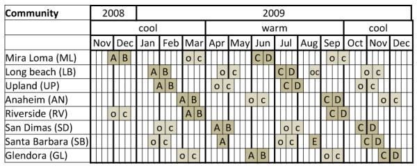
To estimate annual average concentrations, we sampled for a month-long integrated period at two different times of the year, similar to the analyses reported by Xu et al. (2007). Field sampling was conducted in a simultaneous, rotating, community-paired cycle, from December 2008–December 2009, as shown in Table 1. To provide a better estimate of annual average exposure in each community, an additional two waves of four-week sampling were conducted at community central air monitoring stations at off-cycle intervals. Community monitors were operated by the South Coast Management District as part of their standard federal monitoring requirements to test compliance with USEPA National Ambient Air Quality Standards. Due to a wildfire in Santa Barbara during sampling wave B, an additional sampling wave (E) was conducted in Santa Barbara to replace B.
Table 1.
Field sampling schedule. Lettered boxes represent two-week community-wide sampling events, including sampling at regional air monitoring sites; “oc,“ i.e., off-cycle labeled boxes represent additional two-week sampling periods only at central monitoring sites.
|
In each of the eight CHS communities, 26 to 29 sampling sites were selected. These included CHS students’ homes, community regional air monitoring site locations, and neighborhood elementary schools attended by CHS participants. CHS participants’ homes were stratified into the highest one-third and lowest two-thirds of dispersion-model-predicted annual average TRP concentrations, using CALINE-4 (Benson and Pinkerman, 1989). Within these strata, we selected sampling locations defined by high-high, high-low, low-high, and low-low (HH, HL, LH, LL) freeway and arterial traffic sources, respectively. To ensure our selection procedure included locations both under- and over-predicted by dispersion modeling, an equal number of homes were selected having positive or negative residuals from a kriged surface of residuals from a previous spatial regression NOX model (Franklin et al., 2012) developed from a 2005-2006 sampling campaign using Ogawa passive NOX monitors deployed across the same CHS communities.
At participants’ homes, samplers were typically placed in the most open area of the backyard. Sampler inlets were located about 2 m above the ground. Residents were asked to avoid (and/or later document) any combustion activities (use of lawn mowers, barbeques, biomass burning, or smoking) in the immediate vicinity of the sampler. All sampling in each community began simultaneously at midnight and ended exactly four weeks later, with sampling media replaced by field staff two weeks into the month-long integrated sampling period.
2.3 Analysis
2.3.1. Mass Determination
PUF substrates and Teflon filters were pre- and post-weighed with a Mettler MX-5 microbalance after equilibrating for at least 12 hours (48 hours for PUF) under controlled temperature and relative humidity (RH) conditions (70–75 °F and 32–42% RH) in a dedicated balance room. Static charge was removed prior to weighing using a 210Po source. Identical control filters and PUF substrates were interspersed in the weighing process, one for every ten samples. Any observed changes in “control” mass measurements were used to adjust sample masses for differences in humidity at time of weighing. Reference masses, 100 mg for Teflon weightings and 10 mg for PUF weightings, were checked every ten samples. If mass changes exceeded ± 5 μg, samples were re-weighed. Zero checks were performed before each weighing.
2.3.2. Elemental and Organic Carbon
To remove any residual organic carbon (OC), quartz filters were pre-baked at 550° C for twelve hours and stored in Petri dishes lined with aluminum foil similarly treated. After sample collection, each quartz filter was punched (1 cm2) and the punches were dedicated for EC and OC analysis, whereas the remainder of each filter was processed for WSOC. The punch size was factored into final calculations. EC and OC measurements were made using a thermal-optical transmittance method, based on NIOSH Method 5040 (Eller and Cassinelli, 1996). Extraction for WSOC analysis involved placing substrates into pre-cleaned polypropylene test tubes with 10 ml of ultra-pure Type I water (18.2 MΩ), sonicating for 10 minutes, then shaking for 6 hours. Extract was syringe-filtered (pre-cleaned polypropylene 0.45 μm filters, Whatman) and analyzed for total organic carbon using a modification of Standard Methods 5310C (Wisconsin State Laboratory of Hygiene method ESS ORG METHOD 1661.0 rev 1), using a Sievers Portable 900 TOC Analyzer.
2.4. Quality Assurance Procedures
In the laboratory, 10% laboratory blanks (method blanks) were analyzed as part of the routine analyses, and the mean results were subtracted from all results of the same laboratory batch. In the field, 10% of study substrates were collected and treated as travel blanks (identical in substrate preparation, sampler assembly and disassembly, and travel). Median travel blank values for each community and sampling event were subtracted from all samples in their respective group. Co-located duplicate sampling was performed at 10% of the field sampling locations. Tests for erroneous values are described in the Supporting Information (Section S-1).
3. Results
3.1 Quality Assurance Results
Approximately 75% of the 228 originally-designated sampling locations provided two complete months of sampling data. 17 locations yielded only partial sampling coverage due to equipment or power failures. 51 locations required a location change due to participant discontinuation across the year of field activities. Re-located samplers were assigned to locations of similar predicted traffic impact, e.g., HH, HL, etc. As a result, the annual averages including or excluding these moved locations only differed by 0.14% on average for the pollutants presented in subsequent tables and can be derived by taking the average of the warm and cool season values.
Instrument precision was evaluated by comparing collocated measurements (field duplicates), summarized in Table S-1 in the Supplement. The average absolute percent difference between collocated samplers for coarse PM, PM2.5, OC2.5, OC0.2, WSOC2.5, WSOC0.2 was in the range of 4 to 8%. PM0.2, EC0.2, and EC2.5 were higher at 11, 12, and 15%, respectively. In general, precision improved with increasing particle size and/or total mass collected. The collocated precision for WSOC was ±7%.
3.2 Seasonal and Between-Community Differences
To illustrate seasonal and between-community concentration differences in TRP concentrations, box plots are shown in Figures 2 (a) – (l). The first box plot of each community pair represents the cool season; communities are arranged left to right in descending order of cool season EC2.5 concentration. (Tables S-2 and S-3 in the Supplement provide the concentration means and standard deviations by community and season. Figure S-1 in the Supporting Information shows an example of the seasonal pattern when results are ordered by sampling date.)
Figure 2.

Box plots of concentrations by community, with cool season first for each community
In Southern California, weaker daytime sea breezes, lower mixing heights, and stronger nocturnal stagnation conditions occur in the cool season (Oct—Mar) than the warm season (Apr–Sept). This tends to produce higher localized traffic pollution impacts in the cool season for the primary TRPs such as EC2.5 and NOX (Fig. 2 (a) and 2 (c)). Of the pollutants shown, EC2.5 and NOX showed the most distinct seasonal differences. Larger seasonal differences were present where concentrations were highest, such as in Long Beach (LB) and Mira Loma (ML). LB and ML are the two communities most strongly impacted by diesel freight traffic emissions, primarily from seaport operations in LB and from distribution center trucking operations in ML. An exception to the pattern of higher cool season concentrations for primary TRPs occurred in Upland (UP), where cool season sampling coincided with a frontal rainy period of unusually strong regional dilution.
For pollutants with significant contributions from secondary formation such as PM2.5 or WSOC, seasonal differences were less distinct and concentrations were typically as high or higher in the warm season than the cool season. Fig. 2(i) and 2(j) also show reduced variability in PM2.5 and WSOC0.2 concentrations within each community, a characteristic of pollutants of a more regionally uniform nature. Greater regional uniformity is also apparent in coarse PM, Fig. 2 (l), suggesting that resuspended road dust from roadways is a smaller source of coarse PM than regional windblown dusts, with the exception of ML. Other studies in the Los Angeles region have observed greater windblown dust contributions to coarse PM than traffic resuspension, particularly in the more inland areas of the air basin (Pakbin et al., 2010).
It is interesting to note that NOX showed a large decrease in within-community variability in the warm season, shifting to a more regional pollutant. For example, the within-community standard deviation of NOx was 20 and 11 ppb in the cool season for LB and ML, respectively, but only 2.0 and 2.7 ppb in the warm season. Fig. 2 (e) shows the NO2/NOX ratio consistently higher in the warm season, with the exception of SB, indicating greater conversion of NO to NO2 during the higher ozone concentrations of the warm season, one aspect of its regional shift.
3.3 Within-Community Spatial Variability
Fig. 3 (a) – 3 (f) display within-community variability by season, standard deviations (SDs) to show absolute variability, and coefficients of variation (CVs) to show variability relative to the mean. As measures of absolute variation, SDs were usually largest in the cool season for the primary TRPs. Pollutants with significant secondary contributions such as PM2.5 or WSOC2.5 Fig. 3 (e) did not show this pattern.
Figure 3.

Within-community standard deviations, left column, and coefficients of variation, right column, by community, with cool season first for each community. Plotted in order of decreasing cool season EC2.5
Relative variability, as shown by CVs, was also higher for the primary TRPs than secondary pollutants. For example, the average warm and cool season CV for NO was 0.50 and 0.35; for EC2.5 it was 0.22 and 0.18; and for PM2.5 it was on 0.08 and 0.09, respectively. Primary TRPs such as NO and EC tended to have increasing CVs as concentrations decreased, as shown both in the higher warm season CVs and in the slightly upward trend left to right in Fig. 3(b) and 3(d), indicating larger traffic impacts in communities with lower pollution concentrations. By pollutant, CVs appeared to rank along expected differences in localized traffic impacts, i.e., NO > NOX > EC > OC ≈ WSOC > PM2.5.
Seasonal differences in CVs were smaller than for SDs. For the primary TRPs, warm season CVs were often larger due to lower warm season regional and community mean concentrations. For pollutants with significant secondary contribution such as PM2.5 and WSOC2.5, the warm season CV often decreased, reflecting an increase in warm season regional contributions from photochemistry. However, the CVs for these two pollutants were nearly always below 0.2, regardless of season. NOx compounds showed both primary and secondary behavior in their CVs. For example, the CV for NOx decreased from 0.26 to 0.21 from cool to warm season, reflecting some secondary behavior, while NO alone showed an increase, from 0.35 to 0.5.
An additional way to look at relative variability is to calculate the fraction of between-community variance to the sum of between-community and within-community variance, as shown in Figure 4. Figure 4 illustrates that most of the variance occurred between communities (i.e., ratios were less than 0.5) with the exception of warm season NOx and warm season coarse PM. However, it should be noted that a portion of the observed between-community variance resulted from meteorological differences due to non-concurrent sampling.
Figure 4.

Fraction of total measurement variance occurring within each community by pollutant with cool season shown first
3.4. Pollutant Concentration Differences by Traffic Strata
Primary TRPs showed distinct patterns when grouped by traffic strata (LL, LH, HL, HH). To make within-community differences directly comparable, each concentration was adjusted by subtracting the warm or cool season community mean, calculated by averaging all samples within the community. Fig. 5 shows typical patterns for the primary TRPs. Concentrations for NOX compounds and both sizes of EC and OC in the high-freeway-influenced strata (HL and HH), were always higher than those in the low freeway strata (LL and LH), for both cool and warm seasons. These freeway differences were statistically significant (p < 0.05 by Scheffé’s method). Differences tended to be higher in the cool season. High arterial road influences (LH and HH) were also associated with higher pollutant concentrations than corresponding low arterial influences (LL and HL), respectively, but the differences were not statistically significant. Other measured pollutants did not show meaningful patterns of traffic impact (see Figure S-2 in Supporting Information and Table S-4 for pollutant strata means).
Figure 5.

Concentrations after subtracting community seasonal mean values, grouped by roadway strata. “HL” is high freeway, low arterial influence, “LH” is low freeway, high arterial influence, etc. EC2.5 and OC2.5 left, NO and NO2, right.
4. Discussion
Pre-study hypotheses were generally supported by the collected data. Primary pollutants, such as EC and NOX, had higher localized impacts, as shown by traffic strata differences, and freeways showed greater impact than arterial roads, as expected. Moreover, these observable differences were greater in the cool season. We also confirmed greater within-community variability for primary TRPs (as shown by within-community SDs) than secondary pollutants (such as PM2.5 and WSOC), and variability was larger in the cool season. Relative within-community variability, as measured by CV, was higher in the cleaner communities, indicating a larger relative traffic impact in communities with generally lower pollution levels.
Unexpected results were observed for OC and WSOC. OC demonstrated some attributes of a primary pollutant, showing seasonal and traffic strata differences similar to EC. We had expected OC to be more strongly affected by summertime secondary organic aerosol (SOA) formation and for SOA to contribute significantly to WSOC in the warm season. Seasonal ratios were generally similar, however, with the WSOC/OC ratio averaging 0.31 and 0.38 in cool and warm seasons, respectively. The seasonal plot in Supplemental Figure S-3 shows an increase in the WSOC2.5/OC2.5 ratio from early 2009, ranging from 0.15 to 0.35, to summer 2009, where it ranged from 0.25 to 0.45, but the ratio did not decrease in the cool season of late 2009, where it remained about 0.45. For comparison, Figure S-3 shows the corresponding PM2.5 concentrations demonstrating a clear seasonal summertime trend.
Modest seasonal differences in the WSOC fraction of OC suggest that SOA formation may be less seasonally dependent than previous studies (Docherty et al., 2008) suggest. However, we cannot rule out that some of the warm season SOA was lost to volatilization, reducing our warm season ratios. Temperatures averaged 19.4±3.4 °C (SD) in the warm season compared to 14.7±2.3 °C in the cool season, but because backup quartz filters were not routinely used, we cannot confidently evaluate losses. Studies suggest that positive adsorption artifacts exceed the negative volatilization artifacts, on average, for 24-hour or shorter averaging times (Watson et al., 2009), but no evaluations have been made for the two-week sampling intervals employed in the current study.
We were surprised to observe that TRP0.2 was not a better traffic marker than TRP2.5. The components EC0.2 and OC0.2 showed similar traffic strata patterns but less than half of the differences of the 2.5 micron sizes (see Table S-3). Furthermore, PM0.2 mass concentrations were ineffective traffic markers and did not show a consistent pattern of traffic strata differences. This was unexpected, as particle number is strongly elevated near freeways and busy roadways and is considered to be a sensitive marker of traffic emissions. This might suggest that elevated PM concentrations downwind of roadways were reduced more by coagulation, which conserves mass, than by evaporation.
Of the collected data, NOx appeared to be a better marker of traffic than any of the TRP PM components, based on traffic strata differences and within-community variability. NO had the highest within-community variability, followed by NOX, and both of these constituents had within-community CVs at least twice those of EC or OC. Considering that NOX compounds can be measured more cheaply and easily with passive samplers, their utility as a marker of traffic may outweigh the additional costs of sampling PM components. Of the multiple compounds composing NOX, total NOx appeared to be a more stable marker of traffic than NO and showed less seasonal variation. As NO converts more quickly to NO2 during higher warm season ozone concentrations, it produces sharper gradients near traffic, while total NOX is conserved. This was observed downwind of a Los Angeles freeway across various ozone conditions in Rodes and Holland (1981). Thus, NOx may be the preferred traffic marker.
This study represents one of the largest traffic-related particulate matter constituent studies conducted to date, addressing differences in PM composition at both middle (100-500 m) and neighborhood (500 m-4 km) scales as well as urban scale (4-100 km) within a single urban conglomeration. Perhaps the most similar study to date has been the European ESCAPE Project (European Study of Cohorts for Air Pollution Effects). ESCAPE compared spatial variability of PM components over multiple spatial scales. PM2.5, PM10, coarse PM, NOX and NO2, and absorbance (similar to EC) were measured for 14 day intervals, 15 minutes every two hours, in the cold, warm and intermediate seasons, 20 locations per city in 20 cities (36 cities for NOX and NO2), from Oct 2008 to Apr 2011 (Eefstens et al., 2012).
Unfortunately, the ESCAPE study design sampled locations both within and beyond urban core areas (Eeftens et al., 2012), thereby including sampling locations of very low traffic impact and resulting in increased within-city variance. Our study characterized smaller-scale variation within communities across a single large metropolitan region (Los Angeles), but was not able to include locations of very low traffic impact. Therefore, we are unable to directly compare contributions of pollutant variance over shorter and longer scales in the two studies. Furthermore, some ESCAPE cities were large enough to encompass some regional scale (100 to 1000 km) differences, but in our study, regional scale differences were not captured.
These basic differences in sampling design are also reflected in the NO2/NOX ratios. ESCAPE urban background (sites of low traffic) NO2/NOX ratios ranged from 0.51 to 0.72. Our ratios, as shown in Fig 3 (e), were at the low end of this range during the cool season, indicating greater traffic impacts (i.e., higher NO), and at the high end during the warm season, indicating widespread regional NO2. Another reason for differences in spatial variability was likely due to differences in per-vehicle emission rates, which are generally higher in Europe than in the United States (Pouliot et al., 2012). However, a consistent finding in both studies was higher traffic impacts in cleaner locations, which for the ESCAPE study were the cities in northern Europe.
In conclusion, our study found substantial within-community variance in primary TRP concentrations. This suggests a potentially important exposure misclassification issue if central-site monitors are used to predict exposure over geographically large and diverse regional or community areas. Care should be taken, and when possible, estimates should be made, regarding likely within- and between-community variances. However, the within-community variance was smaller than the observed between-community variance. This aspect of spatial variation illustrates the challenge of capturing spatial variability at multiple spatial scales (middle, neighborhood, and urban) within a large urban area: if multiple scales of variation are not captured concurrently, meteorological differences between sampling intervals will make comparisons challenging.
Supplementary Material
Highlights.
Size-resolved PM mass, carbon components and NOx measured spatially
Local traffic impacts observed for elemental and organic carbon and NOx but not PM
Traffic impacts were relatively larger in cleaner communities
No PM components were better markers of traffic than NOx
Acknowledgements
We thank the Harvard School of Public Health (Mike Wolfson, Steve Ferguson, and Petros Koutrakis) and David Vaughn of Sonoma Technology Incorporated for critical support in the development and evaluation of the sampling methodologies, the USC CHS Field Team for their substantial efforts during field sampling, Lisa Grossman for data management, the South Coast Air Quality Management District and school districts who allowed us site access for sampling, and the CHS families who allowed us repeated entry to their homes to conduct the field sampling.
This work was supported by the Southern California Environmental Health Sciences Center (grant # 5P30ES007048) funded by the National Institute of Environmental Health Sciences, the Children’s Environmental Health Center (grant #s 5P01ES009581, R826708-01 and RD831861-01) funded by the National Institute of Environmental Health Sciences and the Environmental Protection Agency, the National Institute of Environmental Health Sciences (grant #s 5P01ES011627, 5R01 ES016535, and 5R03ES014046, and 1K25ES019224-01), the National Heart, Lung and Blood Institute (grant #s 5R01HL061768, 5R01HL076647, 5R01HL087680, and 1RC2HL101651), the Environmental Protection Agency (grant # R831845), and by the Hastings Foundation.
Footnotes
Publisher's Disclaimer: This is a PDF file of an unedited manuscript that has been accepted for publication. As a service to our customers we are providing this early version of the manuscript. The manuscript will undergo copyediting, typesetting, and review of the resulting proof before it is published in its final citable form. Please note that during the production process errors may be discovered which could affect the content, and all legal disclaimers that apply to the journal pertain.
References
- Benson PE, Pinkerman KO. CALINE4, a dispersion model for predicting air pollution concentration near roadways. State of California, Dept. of Transportation, Division of Engineering Services, Office of Transportation Laboratory; 1984. [Google Scholar]
- Brauer M, Hoek G, Van Vliet P, Meliefste K, Fischer PH, Wijga A, Koopman LP, Herman NJ, Jorrit G, Kerkhof M, Joachim H, Bellander T, Brunekreef B. Air pollution from traffic and the development of respiratory infections and asthmatic and allergic symptoms in children. American Journal of Respiratory and Critical Care Medicine. 2002;166(8):1092–1098. doi: 10.1164/rccm.200108-007OC. [DOI] [PubMed] [Google Scholar]
- Cyrys J, Eeftens M, Heinrich J, Ampe C, Armengaud A, Beelen R, Bellander T, Beregszaszai T, Birk M, et al. Variation of NO2 and NOx concentrations between and within 36 European study areas: results from the ESCAPE study. Atmospheric Environment. 2012;62:374–390. [Google Scholar]
- Delfino RJ, Malik S, Sioutas C. Potential role of ultrafine particles in associations between airborne particle mass and cardiovascular health. Environmental Health Perspectives. 2005;113(8):934–946. doi: 10.1289/ehp.7938. [DOI] [PMC free article] [PubMed] [Google Scholar]
- Docherty KS, Stone EA, Ulbrich IM, DeCarlo PF, Snyder DC, Schauer JJ, Peltier RE, Weber RJ, Murphy SM, Seinfeld JH, Grover BD, Eatough DJ, Jimenez JL. Apportionment of primary and secondary organic aerosols in Southern California during the 2005 Study of Organic Aerosols in Riverside (SOAR-1) Environmental Science and Technology. 2008;42(20):7655–7662. doi: 10.1021/es8008166. [DOI] [PubMed] [Google Scholar]
- Eeftens M, Tsai MY, Ampe C, Anwander B, Beelen R, Bellander T, Cesaroni G, Cirach M, Cyrys J, de Hoogh K, et al. Spatial variation of PM2. 5, PM10, PM2. 5 absorbance and PMcoarse concentrations between and within 20 European study areas and the relationship with NO2-Results of the ESCAPE project. Atmospheric Environment. 2012;62:303–317. [Google Scholar]
- Eller PM, Cassinelli ME. NIOSH manual of analytical methods. National Institute for Occupational Safety, Centers for Disease Control and Prevention (US). Public Health Practice Program Office; USGPO; 1996. Elemental carbon (diesel exhaust): Method 5040. (1996) [Google Scholar]
- English P, Neutra R, Scalf R, Sullivan M, Waller L, Zhu L. Examining associations between childhood asthma and traffic flow using a geographic information system. Environmental Health Perspectives. 1999;107(9):761–767. doi: 10.1289/ehp.99107761. [DOI] [PMC free article] [PubMed] [Google Scholar]
- Franklin M, Vora H, Avol E, McConnell R, Lurmann F, Liu F, Penfold B, Berhane K, Gilliland F, Gauderman WJ. Predictors of intra-community variation in air quality. Journal of Exposure Science and Environmental Epidemiology. 2012;22(2):135–147. doi: 10.1038/jes.2011.45. [DOI] [PMC free article] [PubMed] [Google Scholar]
- Gauderman WJ, Avol E, Gilliland F, Vora H, Thomas D, Berhane K, McConnell R, Kuenzli N, Lurmann F, Rappaport E, Margolis H, Bates D, Peters J. The effect of air pollution on lung development from 10 to 18 years of age. New England Journal of Medicine. 2004;351(11):1057–1067. doi: 10.1056/NEJMoa040610. [DOI] [PubMed] [Google Scholar]
- Gauderman WJ, Avol E, Lurmann F, Kuenzli N, Gilliland F, Peters J, McConnell R. Childhood asthma and exposure to traffic and nitrogen dioxide. Epidemiology. 2005;16(6):737–743. doi: 10.1097/01.ede.0000181308.51440.75. [DOI] [PubMed] [Google Scholar]
- Gauderman WJ, Vora H, McConnell R, Berhane K, Gilliland F, Thomas D, Lurmann F, Avol E, Kunzli N, Jerrett M, Peters J. Effect of exposure to traffic on lung development from 10 to 18 years of age: a cohort study. The Lancet. 2007;369(9561):571–577. doi: 10.1016/S0140-6736(07)60037-3. [DOI] [PubMed] [Google Scholar]
- Health Effects Institute, Panel on the Health Effects of Traffic-Related Air Pollution . Traffic-related air pollution: a critical review of the literature on emissions, exposure, and health effects (No. 17) Health Effects Institute; 2010. [Google Scholar]
- Janssen NA, Brunekreef B, van Vliet P, Aarts F, Meliefste K, Harssema H, Fischer P. The relationship between air pollution from heavy traffic and allergic sensitization, bronchial hyperresponsiveness, and respiratory symptoms in Dutch schoolchildren. Environmental Health Perspectives. 2003;111(12):1512–1518. doi: 10.1289/ehp.6243. [DOI] [PMC free article] [PubMed] [Google Scholar]
- Janssen NA, Hoek G, Simic-Lawson M, Fischer P, van Bree L, ten Brink H, Keuken M, Atkinson RW, Anderson HR, Brunekreef B, Cassee FR. Black carbon as an additional indicator of the adverse health effects of airborne particles compared with PM10 and PM2. 5. Environmental Health Perspectives. 2011;119(12):1691–1699. doi: 10.1289/ehp.1003369. [DOI] [PMC free article] [PubMed] [Google Scholar]
- Kavouras IG, Koutrakis P. Use of polyurethane foam as the impaction substrate/collection medium in conventional inertial impactors. Aerosol Science and Technology. 2001;34(1):46–56. [Google Scholar]
- Kim JJ, Smorodinsky S, Lipsett M, Singer BC, Hodgson AT, Ostro B. Traffic-related Air Pollution near Busy Roads The East Bay Children’s Respiratory Health Study. American Journal of Respiratory and Critical Care Medicine. 2004b;170(5):520–526. doi: 10.1164/rccm.200403-281OC. [DOI] [PubMed] [Google Scholar]
- Lee SJ, Demokritou P, Koutrakis P, Delgado-Saborit JM. Development and evaluation of personal respirable particulate sampler (PRPS) Atmospheric Environment. 2006;40(2):212–224. [Google Scholar]
- McConnell R, Berhane K, Yao L, Jerrett M, Lurmann F, Gilliland F, Kuenzli N, Gauderman J. Traffic, susceptibility, and childhood asthma. Environmental Health Perspectives. 2006;114(5):766–772. doi: 10.1289/ehp.8594. [DOI] [PMC free article] [PubMed] [Google Scholar]
- Moore KF, Ning Z, Ntziachristos L, Schauer JJ, Sioutas C. Daily variation in the properties of urban ultrafine aerosol—part I: physical characterization and volatility. Atmospheric Environment. 2007;41(38):8633–8646. [Google Scholar]
- Nicolai T, Carr D, Weiland SK, Duhme H, Von Ehrenstein O, Wagner C, Von Mutius E. Urban traffic and pollutant exposure related to respiratory outcomes and atopy in a large sample of children. European Respiratory Journal. 2003;21(6):956–963. doi: 10.1183/09031936.03.00041103a. [DOI] [PubMed] [Google Scholar]
- Pakbin P, Hudda N, Cheung KL, Moore KF, Sioutas C. Spatial and Temporal Variability of Coarse (PM10– 2.5) Particulate Matter Concentrations in the Los Angeles Area. Aerosol Science and Technology. 2010;44(7):514–525. [Google Scholar]
- Peters JM, Avol E, Navidi W, London SJ, Gauderman WJ, Lurmann F, Linn WS, Margolis H, Rappaport E, Gong H, Thomas DC. A study of twelve southern California communities with differing levels and types of air pollution I. Prevalence of respiratory morbidity. American Journal of Respiratory and Critical Care Medicine. 1999;159(3):760–767. doi: 10.1164/ajrccm.159.3.9804143. [DOI] [PubMed] [Google Scholar]
- Pouliot G, Pierce T, Denier van der Gon H, Schaap M, Moran M, Nopmongcol U. Comparing emission inventories and model-ready emission datasets between Europe and North America for the AQMEII project. Atmospheric Environment. 2012;53:4–14. [Google Scholar]
- Rodes CE, Holland DM. Variations of NO, NO2 and O3 concentrations downwind of a Los Angeles freeway. Atmospheric Environment. 1981;15(3):243–250. [Google Scholar]
- van Vliet P, Knape M, de Hartog J, Janssen N, Harssema H, Brunekreef B. Motor vehicle exhaust and chronic respiratory symptoms in children living near freeways. Environmental Research. 1997;74(2):122–132. doi: 10.1006/enrs.1997.3757. [DOI] [PubMed] [Google Scholar]
- Venn A, Lewis S, Cooper M, Hubbard R, Hill I, Boddy R, Bell M, Britton J. Local road traffic activity and the prevalence, severity, and persistence of wheeze in school children: combined cross sectional and longitudinal study. Occupational and Environmental Medicine. 2000;57(3):152–158. doi: 10.1136/oem.57.3.152. [DOI] [PMC free article] [PubMed] [Google Scholar]
- Venn AJ, Lewis SA, Cooper M, Hubbard R, Britton J. Living near a main road and the risk of wheezing illness in children. American Journal of Respiratory and Critical Care Medicine. 2001;164(12):2177–2180. doi: 10.1164/ajrccm.164.12.2106126. [DOI] [PubMed] [Google Scholar]
- Watson JG, Chow JC, Chen LWA, Frank NH. Methods to assess carbonaceous aerosol sampling artifacts for IMPROVE and other long-term networks. Journal of the Air and Waste Management Association. 2009;59(8):898–911. doi: 10.3155/1047-3289.59.8.898. [DOI] [PubMed] [Google Scholar]
- Watson JG, Chow JC, DuBois DW, Green MC, Frank NH, Pitchford ML. Guidance for network design and optimal site exposure for PM2.5 and PM10. U.S. Environmental Protection Agency, Research Triangle Park, NC; 1997. Report No. EPA-454/R-99-022. [Google Scholar]
- Wjst M, Reitmeir P, Dold S, Wulff A, Nicolai T, von Loeffelholz-Colberg EF, Von Mutius E. Road traffic and adverse effects on respiratory health in children. British Medical Journal. 1993;307(6904):596. doi: 10.1136/bmj.307.6904.596. [DOI] [PMC free article] [PubMed] [Google Scholar]
- Xu X, Brook JR, Guo Y. A Statistical Assessment of Saturation and Mobile Sampling Strategies to Estimate Long-Term Average Concentrations across Urban Areas. Journal of the Air and Waste Management Association. 2007;57(11):1396–1406. [PubMed] [Google Scholar]
- Zhu Y, Hinds WC, Kim S, Shen S, Sioutas C. Study of ultrafine particles near a major highway with heavy-duty diesel traffic. Atmospheric Environment. 2002;36(27):4323–4335. [Google Scholar]
- Zmirou D, Gauvin S, Pin I, Momas I, Sahraoui F, Just J, Le Moullec Y, Bremont F, Cassadou S, Reungoat P, et al. Traffic related air pollution and incidence of childhood asthma: results of the Vesta case-control study. Journal of Epidemiology and Community Health. 2004;58(1):18–23. doi: 10.1136/jech.58.1.18. [DOI] [PMC free article] [PubMed] [Google Scholar]
Associated Data
This section collects any data citations, data availability statements, or supplementary materials included in this article.