Active wide-field illumination for high-throughput fluorescence lifetime imaging

Abstract

Wide-field fluorescence lifetime imaging allows for fast imaging of large sample areas at the cost of low sensitivity to weak fluorescence signals. To overcome this challenge, we developed an active wide-field illumination (AWFI) strategy to optimize the impinging spatial intensity for acquiring optimal fluorescence signals over the whole sample. We demonstrated the ability of AWFI to accurately estimate lifetimes from a multiwell plate sample with concentrations ranging over two orders of magnitude. We further reported its successful application to a quantitative Förster resonance energy transfer lifetime cell-based assay. Overall, this method allows for enhanced accuracy in lifetime-based imaging at high acquisition speed over samples with large fluorescence intensity distributions.

Fluorescence lifetime imaging (FLI) is a quantitative method employed to measure alterations in the fluorescence decay of fluorophores in living cells. FLI has been widely used to investigate changes in cellular environment, metabolic activity, and protein–protein interactions via Förster resonance energy transfer (FRET) [1]. FLI is poised to play an increasingly important role in drug discovery and cell biology studies. For instance, FLI has been recently implemented in a multiwell plate reader configuration for high content analysis and high-throughput screening to image FRET assays [2].

However, the large dynamic range of fluorescence emission intensities collected over a large sample area is one of the challenges in quantitative FLI studies. For example, the dynamic range of fluorescence signals over a multiwell plate can depend on fluorophore concentrations, FRET efficiencies (quenching), relative protein expressions, cellular environments, etc. If the fluorescence intensity variations fall outside of the acquisition system dynamic range, the strongest signals are saturated and/or the weakest signals are lost. As the fluorescence lifetime estimation is based on fitting the measured intensity decay curve to an appropriate exponential model, the estimation of the lifetime values becomes unreliable due to poor photon count statistics in low intensity areas [3].

To overcome this challenge, spatial control of illumination energy on the sample has been devised, such as controlled light exposure (CLE) method [4] and active illumination (AI) method [5]. These techniques have been implemented in commercial systems and in the academia for advanced microscopy applications with great success. For instance, Nikon Instrument has integrated CLE in a commercial confocal microscope to reduce phototoxicity and photobleaching by shutting off illumination for the background and the regions with an adequate signal-to-noise ratio (SNR) via a feedback system during a given exposure time. Moreover, CLE has been applied successfully to stochastic optical reconstruction microscopy (STORM) and programmable array microscopes. In AI method, the laser power is adjusted to maintain a constant signal level per pixel in the image to improve the SNR and weak-signal sensitivity. AI has been incorporated into confocal and two-photon microscopes. CLE and AI have been implemented in raster scanning imaging systems (SIS). However, SIS is inherently far slower than nonscanning wide-field imaging systems, limiting their use for high-throughput applications.

In this study, we implemented AI into nonscanning wide-field FLI applied to multiwell plate imaging by adjusting not only the overall laser power but also the spatial distribution of the wide-field illumination via a spatial light modulator. This method aims at mitigating the range of emitted fluorescence intensities to improve the accuracy of fluorescence decay curve fitting and SNR. This is achieved by balancing iteratively the fluorescence signals at the maximum of the fluorescence decay curve over the illumination area until the photon counts reach the limit of the detector. This method not only improves the SNR and weak-signal sensitivity for fluorescence lifetime analysis, but also reduces the acquisition time and photobleaching.

We implemented our active wide-field illumination (AWFI) method in a time-domain FLI system based on a gated intensified CCD (ICCD) detection described in detail in [6]. Instead of a picoprojector, a digital micro-mirror device (DMD, DLP Discovery 4100 Kit and D2D module, Texas Instruments Inc.) is used as a spatial light modulator to create a spatial distribution of light beams with a resolution of 1024 × 768 pixels and 256 grayscale levels. The overall laser power is adjustable using a computer-controlled variable attenuator (Application Note 30, Newport) based on the combination of a half-wave plate and a polarizer with a closed loop feedback-control system. The laser beam exiting the power control assembly is coupled into a 400 μm multimode fiber (NA = 0.22), and then it is collimated and focused into the integrator rod of the optical module (S2+ optics, Texas Instruments Inc.). The transmitted fluorescence signal from the sample is spectrally filtered by an emission bandpass filter (FF01-720/13-25 for Alexa Fluor 700 at 695 nm as an excitation wavelength, FF01-832/37-25 for Cardiogreen dye at 780 nm as an excitation wavelength, Semrock Inc.) and detected by the ICCD (PicoStar HR, LaVision GmbH). ICCD allows the measurement of a maximum of 2¹² photons with a spatial resolution of 1376 × 1040 pixels.

The 2D time-resolved spatial images are acquired at the emission wavelength. The spatial image at the maximum (peak) of the fluorescence decay curve is identified and AWFI is applied at this time position (time gate). The AWFI iterative procedure consists in optimizing the illumination pattern until the photon counts of the fluorescence signal reach the desired photon counts set by user at any given position over the full sample. Before AWFI, an excitation image is measured to create a binary mask by image segmentation and connected components labeling. The binary mask is applied to the initial uniform pattern to restrict the signals to the observed wells.

The AWFI optimization algorithm flowchart at the nth iteration is shown in Fig. 1(a). The superscript (n) and (n + 1) represent the nth and (n + 1)th iteration, respectively. For initialization, the current laser power, the maximum laser power, the final desired photon count N_f (typically <2¹² for 12-bit CCD), and the grayscale pattern are provided as input parameters. γ is defined as the maximum laser power divided by the current laser power. If γ > 1, the 2D spatial image at maximum is read from the experimental data. N_ave is the average of the maximum photon counts from each individual well. N is defined as an intermediate desired photon count to avoid extreme values caused by N_f. If N_ave < N_f, let N equal N_ave. Note that the laser power and gray levels are proportional to the photon counts [see Fig. 1(b)]. Therefore, for each pixel at (i,j) at the nth iteration, P⁽ⁿ⁺¹⁾ can be obtained from the following equations:

$$A^{(n)}(i,j)=\frac{N^{(n)}}{S^{(n)}(i,j)}·P^{(n)}(i,j),(A^{(n)}(i,j)\le {\gamma }^{(n)}),$$ (1)

$$P^{(n+1)}(i,j)=\frac{A^{(n)}(i,j)}{{\alpha }^{(n)}}.$$ (2)

Here, P⁽ⁿ⁾ is the normalized illumination grayscale pattern at the nth iteration. S is a 2D spatial image at the maximum. A represents the relative change in laser powers (or gray levels) required at each position on the pattern to achieve N. α is a laser power modification factor and is determined by the average of the maximum values from each individual well on A. P⁽ⁿ⁺¹⁾ is the updated illumination pattern for the (n + 1)th iteration. For experimental implementation [see Fig. 1(c)], the updated pattern is used and the overall laser power is adjusted by α. This process is repeated until γ = 1 or N_ave ≥ N_f, or α = 1. Note that median value can also be used for calculating N_ave and α to avoid extreme values. In our work, no obvious differences in pattern optimization between median and average values were observed.

Fig. 1.

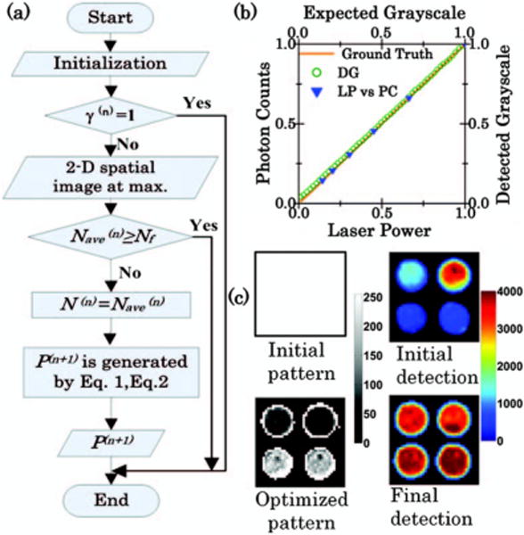
(a) AWFI algorithm flowchart at the nth iteration. (b) Comparison of photon counts (PC) versus laser power (LP), and comparison of detected grayscale (DG) versus expected grayscale. (c) One example of AWFI procedure used for fluorescence measurement. The initial illumination pattern and final optimized pattern are shown on the left with a 0–255 grayscale bar. The corresponding fluorescence detected images are shown on the right with a 0–4000 colorbar.

To establish the robustness and convergence rate of the iterative optimization algorithm, three initial patterns with different spatial intensity distributions were used and optimized toward homogenous field detection [uniform, gradient, and random initial patterns shown in Figs. 2(a)–2(c), respectively]. These three patterns were projected on a piece of diffuse paper laid on the imaging stage. The uniformity is defined as the following expression:

$$\text{Uniformity}=100·(1-\frac{\sigma }{N_m}).$$ (3)

Here, σ is the standard deviation of photon counts. N_m is the mean photon counts in the field of view (FOV). Algorithm stability was validated by N_m, γ, and uniformity versus different iteration numbers as shown in Figs. 2(d) and 2(e). These parameters converged after 4 iterations for the uniform pattern, 4 iterations for the gradient pattern, and 5 iterations for the random pattern. The uniformity is up to 93% after the optimization process for the three types of patterns.

Fig. 2.

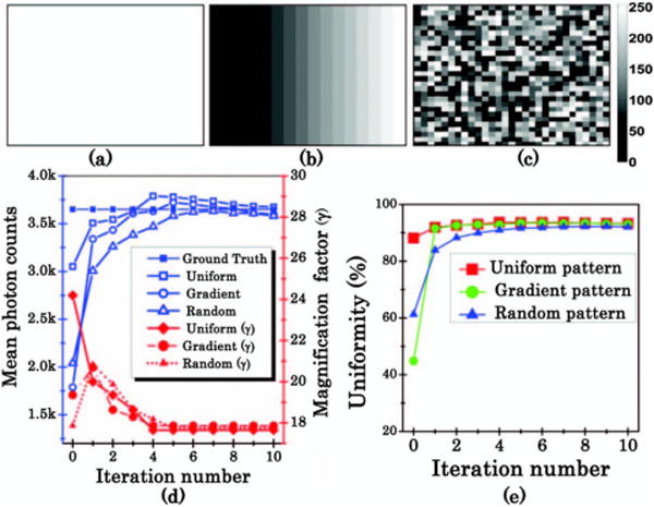
(a) Uniform pattern. (b) Gradient pattern. (c) Random pattern. (d) and (e) Comparison of N_m, γ, and uniformity versus different iteration numbers in. Colorbar, 0–255.

AWFI was applied to fluorescence imaging in multiwell settings. Cardiogreen dye (I2633, Sigma-Aldrich) was dissolved in 50% ethanol at different concentrations: 5, 15, 45, 125, 350, and 1000 nM. The optimized pattern to capture optimal fluorescence signal over the sample was obtained after 4 iterations and in less than a minute. There are 6 wells in one FOV for this specific experiment.

The wells with 5, 15, and 45 nM were not resolved when using nonoptimized pattern (homogenous wide-field illumination) as shown in the original image [Fig. 3(a)]. After AWFI, all the wells in the FOV were resolved with photon counts up to 3600 as shown in Fig. 3(b). Lifetime estimation was performed on each individual well before and after AWFI. As expected, fluorescence decay curve fitting was not accurate when the fluorescence signals were too weak (<100 counts such as in 5 to 45 nM wells prior to AWFI), but the lifetimes were in excellent agreement with the ground truth after AWFI as shown in Fig. 3(c) (within ±5 ps). The ground truth lifetime was obtained by optimizing and acquiring a fluorescence signal on each individual well, one at a time. For the 5 nM well, the lifetime estimates were 357 ± 4 ps (mean ± standard deviation) for the ground truth, 349 ± 46 ps before AWFI, and 355 ± 8 ps after AWFI. The total bias, estimated as the ratio of the two times standard deviation to the mean value, was 2.2%, 26%, and 4.5%, respectively. After AWFI, the fluorescence intensity can be corrected using the optimized pattern intensity distribution to retrieve the relative brightness of each well [see Fig. 3(d)]. The corrected fluorescence intensity shows better linearity (slope = 0.001, R² = 0.99) to different concentrations, especially at low concentrations. Post processing intensity correction allows performing quantitative fluorescence intensity comparisons within the same FOV. These results demonstrate that AWFI can improve the accuracy of intensity-based and lifetime-based quantitative estimation.

Fig. 3.

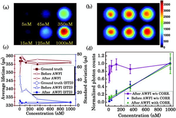
Fluorescence intensity image at the maximum of decay curve (a) without AWFI procedure and (b) with AWFI procedure. (c) Comparison of average estimated lifetime and standard deviation (STD) of lifetimes for each well. (d) Comparison of the fluorescence intensities with and without (w/o) correction (CORR.) versus different concentrations before and after AWFI. Linear regression applied to fluorescence intensity before AWFI w/o CORR. and after AWFI with CORR. to different concentrations yields R² = 0.96 and R² = 0.99, respectively.

Next, we applied the approach to a cell-based FRET assay. We especially focused on estimating the FRET donor fraction (FDF) as estimated by biexponential lifetime analysis (fraction of short lifetime component). In previous work, we have shown that FRET efficiency, which is linearly dependent on FDF, is positively dependent on acceptor to donor ratios (A:D) and independent of acceptor levels in clustered interactions [7,8]. Though, in a fluorescence FRET assay, brightness is determined by donor concentration and quenching (FRET efficiency). Here, we applied AWFI to visualize human transferrin molecules (Tfn) labeled with a near-infrared FRET pair (Alexa Fluor 700-Alexa Fluor 750) in Madin–Darby canine kidney (MDCK) cells expressing human transferrin receptor and T47D cells (human ductal breast epithelial tumor cell line) as described previously for visible wavelengths [8]. Six different A:D ratios (0:1 to 3:1) at various total amount of Tfn ([Tfn], ½[Tfn]) were employed to establish FRET efficiency and sensitivity in these two cell lines. The results are summarized in Fig 4. A subset of the data is tabulated in Table 1 for convenience. As shown in Fig. 4(d), a consistent linear relationship between FDF and A:D ratios can be obtained with AWFI for different cell types and concentrations over a broad range of A:D ratios within a wide-field acquisition protocol. Conversely, the FDF estimated before AWFI was not demonstrating the well-established behavior of clustered interactions when increasing A:D ratios. Overall, the relative error in estimating the FDF using AWFI was smaller than 6% in all the 18 wells imaged. These results demonstrate the potential of AWFI to provide lifetime-based estimation for quantitative FRET analysis.

Fig. 4.

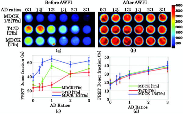
Fluorescence intensity image at the maximum of decay curve (a) without AWFI procedure and (b) with AWFI procedure. Comparison of FDF versus different A:D ratios (c) without AWFI procedure and (d) with AWFI procedure.

Table 1.

FDF Estimates for a Subset of 6 Wells^a

		MDCK (1/2[Tfn])		T47([Tfn])
A:D	Ground Truth	NOPT	AWFI	NOPT	AWFI
0:1	18	39 (117%)	17 (6%)	24 (33%)	18 (0%)
1:3	22	49 (123%)	23 (5%)	25 (14%)	22 (0%)
3:1	38	62 (63%)	40 (5%)	46 (21%)	37 (3%)

^aThe results are provided in percentage. The relative error between the estimated FDF and ground truth are reported in parenthesis in percentage. NOPT stands for nonoptimized.

The overall time of acquisition and optimization for the layout of Fig. 4 was 3 min (18 wells in one FOV). Note that 3 min is for the whole imaging session: all the wells and with the iterative optimization. In our implementation, the FOV is adjustable to match the full size of the plate. It can be scaled to image one well or all the wells simultaneously. The iterative illumination optimization was achieved within 5 iterations (4 in average) for all cases investigated. The overall time of acquisition broke down into: ➀ Fluorescence acquisition for optimization, 1 time gate × 800 ms × 5 iterations = 4 s. ➁ Optimal fluorescence measurement, 120 time gates × 800 ms = 96 s. ➂ IRF measurement, 45 time gates × 50 ms = 2.25 s. ➃ Optimization calculation, 19 s. This is a significantly faster acquisition time than the one reported by recent FLI plate readers [9–12].

For instance, Talbot et al. [9] achieved an acquisition time of ~16 min to read a 96-well plate (10 s/FOV, FOV = 309 × 235 μm). However, this reported acquisition time doesn’t include the prefind scan time that is required for finding cells of interest. Prefind scan not only increases the acquisition time, but also increases the light dose on the sample. Alibhai et al. [10] reported 30 min prefind acquisition time to get 4 FOVs per well for FLI assay prior to the data acquisition. Moreover, these minimum acquisition times were reported for FLI assay, not FRET assay. FRET assay takes even longer total procedure time (acquisition time + prefind scan). Talbot et al. [9] reported 30 min for a 96-well plate without including the prescan time and Alibhai et al. [10] reported 48 min without including the prescan time.

Additionally, our acquisition protocol aimed at acquiring dense temporal data sets for optimal fitting. In Fig. 4, 120 time gates were acquired (4.8 ns window, 40 ps time steps, 300 ps gate width). Talbot et al. [9], Alibhai et al. [10], and Esposito et al. [11] used rapid lifetime determination for lifetime fitting. They used 2 time gates for monoexponential fitting and 6 time gates for biexponential fitting. Grecco et al. [12] used phasor analysis for lifetime fitting. Reducing the number of acquired gates linearly reduces the acquisition time. If only 6 time gates are acquired, the overall imaging procedure will reduce to 30 s with acquisition time less than 10 s for optimal fluorescence measurements (step ➀+➁) over 96 wells using AWFI. This acquisition time is extremely attractive for FLI applications, especially high-throughput FRET assays.

Another important aspect of fluorescence imaging is the issue of photobleaching, especially when multiple exposures per FOV are employed. For the typical experimental settings employed herein, the maximum input laser power at 695 nm as an excitation wavelength was ~90 mw over the full FOV. For the 6-well configuration, the maximum light dose delivered was 0.3 J/cm² (32 mm × 25 mm FOV). For the 18 wells imaging session, the maximum light dose was 0.62 J/cm². Note that these are the theoretical maximum light dose as it corresponds to cases where all pixels in the illumination patterns are at maximum (255 gray level). In any case, both light doses are significantly smaller than typical photobleaching values or phototoxic thresholds [13].

In summary, we have developed a new approach to perform an accurate quantitative wide-field fluorescence imaging over a heterogeneous sample. We applied this new approach, AWFI, to lifetime sensing and validated the method stability experimentally. Since AWFI is able to obtain homogenous fluorescence intensity distribution, it can be applied to both lifetime imaging and fluorescence intensity measurements. We demonstrated the potential of the technique with a macroFRET assay application in multiwell settings with different cells line and labeling concentrations. AWFI can be implemented in automated FLI multiwell plate reader for high content analysis and high-throughput screening by providing high acquisition speed, high SNR, and high precision of fluorescence lifetime fitting. AWFI can also be easily implemented to any wide-field imaging system equipped with a spatial light modulator and programmable array microscope. Moreover, it can be implemented in preclinical settings to mitigate the high dynamic range observed in transmission through the animal body [14].

References

- 1.Becker W. J Microsc. 2012;247:119. doi: 10.1111/j.1365-2818.2012.03618.x. [DOI] [PubMed] [Google Scholar]
- 2.Jones PB, Herl L, Berezovska O, Kumar AT, Bacskai BJ, Hyman BT. J Biomed Opt. 2006;11:054024. doi: 10.1117/1.2363367. [DOI] [PubMed] [Google Scholar]
- 3.Kollner M, Wolfrum J. Chem Phys Lett. 1992;200:199. [Google Scholar]
- 4.Hoebe RA, Van Oven CH, Gadella TW, Jr, Dhonukshe PB, Van Noorden CJ, Manders EM. Nat Biotechnol. 2007;25:249. doi: 10.1038/nbt1278. [DOI] [PubMed] [Google Scholar]
- 5.Chu K, Lim D, Mertz J. Biomed Opt Express. 2010;1:236. doi: 10.1364/BOE.1.000236. [DOI] [PMC free article] [PubMed] [Google Scholar]
- 6.Venugopal V, Chen J, Intes X. Biomed Opt Express. 2010;1:143. doi: 10.1364/BOE.1.000143. [DOI] [PMC free article] [PubMed] [Google Scholar]
- 7.Wallrabe H, Bonamy G, Periasamy A, Barroso M. Mol Biol Cell. 2007;18:2226. doi: 10.1091/mbc.E06-08-0700. [DOI] [PMC free article] [PubMed] [Google Scholar]
- 8.Periasamy A, Wallrabe H, Chen Y, Barroso M. Methods Cell Biol. 2008;89:569. doi: 10.1016/S0091-679X(08)00622-5. [DOI] [PubMed] [Google Scholar]
- 9.Talbot CB, McGinty J, Grant DM, McGhee EJ, Owen DM, Zhang W, Bunney TD, Munro I, Isherwood B, Eagle R, Hargreaves A, Dunsby C, Neil MA, French PM. J Biophotonics. 2008;1:514. doi: 10.1002/jbio.200810054. [DOI] [PubMed] [Google Scholar]
- 10.Alibhai D, Kelly DJ, Warren S, Kumar S, Margineau A, Serwa RA, Thinon E, Alexandrov Y, Murray EJ, Stuhmeier F, Tate EW, Neil MAA, Dunsby C, French PMW. J Biophotonics. 2013;6:398. doi: 10.1002/jbio.201200185. [DOI] [PMC free article] [PubMed] [Google Scholar]
- 11.Esposito A, Dohm CP, Bahr M, Wouters FS. Mol Cell Proteomics. 2007;6:1446. doi: 10.1074/mcp.T700006-MCP200. [DOI] [PubMed] [Google Scholar]
- 12.Grecco HE, Roda-Navarro P, Girod A, Hou J, Frahm T, Truxius DC, Pepperkok R, Squire A, Bastiaens PI. Nat Methods. 2010;7:467. doi: 10.1038/nmeth.1458. [DOI] [PubMed] [Google Scholar]
- 13.Manders EM, Visser AE, Koppen A, de Leeuw WC, van Liere R, Brakenhoff GJ, van Driel R. Chromosom Res. 2003;11:537. doi: 10.1023/a:1024995215340. [DOI] [PubMed] [Google Scholar]
- 14.Venugopal V, Intes X. J Biomed Opt. 2013;18:036006. doi: 10.1117/1.JBO.18.3.036006. [DOI] [PMC free article] [PubMed] [Google Scholar]