Interactive MRI Segmentation with Controlled Active Vision

Abstract

Partitioning Magnetic-Resonance-Imaging (MRI) data into salient anatomic structures is a problem in medical imaging that has continued to elude fully automated solutions. Implicit functions are a common way to model the boundaries between structures and are amenable to control-theoretic methods. In this paper, the goal of enabling a human to obtain accurate segmentations in a short amount of time and with little effort is transformed into a control synthesis problem. Perturbing the state and dynamics of an implicit function’s driving partial differential equation via the accumulated user inputs and an observer-like system leads to desirable closed-loop behavior.

Using a Lyapunov control design, a balance is established between the influence of a data-driven gradient flow and the human’s input over time. Automatic segmentation is thus smoothly coupled with interactivity. An application of the mathematical methods to orthopedic segmentation is shown, demonstrating the expected transient and steady state behavior of the implicit segmentation function and auxiliary observer.

I. Introduction

A ubiquitious problem in medical image processing is segmentation, where salient objects are to be marked within an image. Scanning technologies such as Magnetic-Resonance (MRI) and X-Ray Computed Tomography (CT) yield three-dimensional volumetric images which are then viewed by a doctor for diagnosis or treatment planning. Typically, only a particular anatomic region or organ is of interest; segmentation refers to the process of labeling individual voxels according to tissue type. Performing this classification relies on both the observed intensities and some prior anatomical knowledge on the part of either a human expert or automated algorithm.

Due to the hazardous effects of x-ray radiation in CT scans, it is often desirable to use MRI scanning, even for bone injuries. Unlike CT scans, which give a high reflection from bone and penetrate through soft-tissue, MRI volumes contain return signals from essentially all of the soft-tissue and fluids. While the information needed for segmentation is embedded in the resulting voxels, there is not, in general, a simple set of thresholds to extract a structure in all slices. The distribution of intensity values arising from a particular structure may vary signficantly within the structure, and additionally overlap the distributions of other structures.

High-quality segmentation can certaintly be accomplished by an expert human user manually tracing each slice in the volume. This is usually impractical due to time constraints and discourages high-resolution scanning to keep the number of volume slices manageable. Automated techniques for segmenting such data has been the subject of much recent medical computing literature, with particular emphasis on brain and heart segmentation [1]–[3].

A. Automatic Segmentation: Methods and Limitations

Automatic techniques for segmentation generally incoporate one or both of the following concepts. First, the notion of a salient structure is often quantifiable in terms of a functional that evaluates how different (in terms of image and gradient statistics) a region is its surroundings. This leads, for example, to iterative schemes for separating of regions based on different mean intensities [4] or more generally differences in distributions [5]. Second, there are often plenty of examples of a segmentation result done by an expert user, enabling the user of shape-priors and related knowledge-based techniques [6]–[8].

Consider the problem of segmenting a knee joint for the clinical goal of diagnosing an anterior-cruciate ligament (ACL) tear and determining optimal surgical insertion points. The difficulty in separating regions based on intensity statistics is illustrated in Fig. 1. For a large structure in MRI, an intensity value arising within will almost certainly also exist in the exterior. Complex distribution models that incorporate a joint distribution of textures, gradients, and other higher order data can improve the result for most of the bone surface. However, the most relevant sites for surgical repair are growth-plate junctions and ligament insertion points; these are also the most statistically complex and patient-specific. Thus, it is quite difficult in practice to formulate a useful higher-order model.

Fig. 1.

Bone tissues within one MRI slice have overlapping intensity histograms. Inhomogeneity of a particular bone tissue across MRI slices is also signficant. There is not, in general, a function to map intensity values to anatomical regions.

B. Background: Interactive Segmentation

While statistical descriptors of anatomic regions and prior shape knowledge are powerful concepts towards increased automation of segmentation, they have not significantly displaced the expert human as the primary generator of volume segmentations. In addition to reasons of insufficient data for unique juvenile and trauma cases, there is a great deal of mistrust both from patients and doctors towards fully automatic medical analysis. Instead, there has been a recent drive towards semiautomatic image processing. Ideally, such an interactive system should be designed as to enable a user to create excellent segmentation results with a minimal amount of time and effort.

Interactive segmentation as presented here is motivated by experiences with existing software tools, such as 3D-Slicer [9], [10] and Seg3D [11]. Typically, a user will first attempt to use automatic segmentation with partial success. They will then find a combination of manual editing and re-processing one small subdomain at a time to get a satisfactory result. The novel contribution in this paper is a modeling formulation that represents interactive segmentation as a feedback system, thus enabling a principled merging of automated methods and user input. Having this framework in place allows the tools of control theory to be invoked for system analysis and design.

C. Notation and Organization

The remainder of this paper is as follows: a general model of an interactive segmentation system is presented in Section II. An approach for designing specific control signals and interaction structure are presented in Section III, with the sample application to segmentation of orthopedic MRI data in Section IV. To conclude, final remarks and some interesting directions for future work are given in Section V.

Imaging-Specific Definitions

Due to the multidisciplinary nature of the present work, several clarifications and definitions are in order. The term finesse refers to the level of attentiveness and care with which a user applies input, e.g. with a computer mouse, while manually tracing boundaries in the image. MRI volume imagery is acquired as a sequence of planar slices, with each discrete spatial grid point called a voxel. During segmentation and diagnostics, visualization is the mapping of image intensities in each voxel, current labelling assignments, and a geometric transformation to the user’s screen.

Mathematical Notation

Define Ω to be the three-dimensional volume domain and x a coordinate in Ω. Labeling assignments are represented with an implicit function ϕ(x, t) : ℝ³ × [0, t) → ℝ. As illustrated in Fig. 3, boundaries between regions of interest are represented as level sets where ϕ(x, t) = C. Differentiating with respect to time, ϕ_t = −∇ϕ · f, where f is a data-driven vector field controlling how ϕ changes over time. Since the normal vector N to a level set is given by $\mathbf{N}=-\frac{\nabla \varphi }{\Vert \nabla \varphi \Vert }$, we have that ϕ_t = ‖∇ϕ‖N · f.

Fig. 3.

From the initial implicit curve ϕ(x, 0) = 0, ϕ follows a gradient flow that minimizes an image-driven functional.

II. System Structure

In the following subsections, consituent parts of an interactive medical volume segmentation system are presented. Gradient flows corresponding to functional minimization in image processing are reviewed in Section II-A. Methods by which these flows can be perturbed and controlled via interaction are described in Section II-B, The next Section III uses the model to synthesize a useful set of control signals.

A. Image Segmentation with Gradient Flows

Dynamics that we seek to control result from gradient flows of image-dependent functionals in image segmentation. Data enters via the time-independent but spatially-varying image I(x). At each point in the image domain, a function g(ϕ, I) assigns the data-driven cost while regularity and smoothness are imposed on ϕ and ∇ϕ. The class of functionals considered in this paper lead to nominal, or fully-automatic, dynamics of ϕ denoted as ϕ_t = G(ϕ, I). A central theme in image analysis with partial differential equations is the design of G(ϕ, I) to either minimize a meaningful energy or simply exhibit some desirable properties as ϕ goes towards steady-state; see for example [12], [13] and the references therein.

Example Consider the following, where g(·) and ‖∇ϕ‖ encode data and smoothness, respectively:

$$ℰ(\varphi )={\int }_{\mathrm{\Omega }}g(\varphi ,I){\Vert \nabla \varphi \Vert }_{2}d\mathrm{\Omega }.$$ (1)

An expression for ϕ_t comes from differentiating under the integral and integrating by parts¹:

$$\frac{d}{dt}ℰ={\int }_{\mathrm{\Omega }}{\varphi }_t\frac{\partial g}{\partial \varphi }\Vert \nabla \varphi \Vert +\frac{g\nabla \varphi ·\nabla {\varphi }_t}{\Vert \nabla \varphi \Vert }d\mathrm{\Omega },$$ (2)

$$={\int }_{\mathrm{\Omega }}{\varphi }_t[\frac{\partial g}{\partial \varphi }\Vert \nabla \varphi \Vert -\nabla ·\frac{g\nabla \varphi }{\Vert \nabla \varphi \Vert }]d\mathrm{\Omega }.$$ (3)

Defining $\mathbf{N}=\frac{\nabla \varphi }{\Vert \nabla \varphi \Vert }$ and $\kappa =\nabla ·\frac{\nabla \varphi }{\Vert \nabla \varphi \Vert }$, the gradient flow for ϕ_t is

$${\varphi }_t=-g_{\varphi }(\varphi ,I)\Vert \nabla \varphi \Vert +\nabla g·\mathbf{N}+\kappa g.$$ (4)

Functions of this form are popular in algorithms for segmentation, denoising, and pose estimation [13].

Remark Since ϕ_t = G(ϕ, I) arises from a functional of choice ℰ, it is straighforward to ensure that mild conditions are satisfied by G(·) through modifications of ℰ. In Section II-B, it shall be assumed that G and its gradient are bounded in absolute value to establish the negativity of a Lyapunov functional.

B. Interaction: State and Dynamics Perturbation

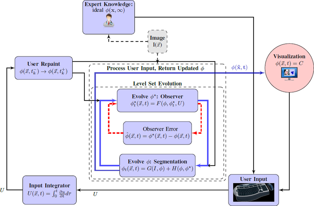
A general overview of the interactive image segmentation model is shown in Section II and Fig. II. From a user’s perspective, it is necessary to be able to apply sudden changes to the implicit segmentation function ϕ(x, t). This is modelled by ϕ transitioning from ϕ(x, t⁻) to ϕ(x, t⁺) driven by a step function. Such a jump occurs at a countably finite number of times, denoted t_k. U(x, t) is a time integral of the user’s input,

$$U(\mathbf{x},t)={\int }_0^t\frac{\partial U}{\partial t}d\tau ,$$ (5)

and it sets the impulse-driven changes in ϕ at input times t_k:

$$\frac{\partial U}{\partial t}=\{\begin{array}{cc}\varphi (\mathbf{x},t_k^{+})-\varphi (\mathbf{x},t_k^{-})\hfill & \text{for}{t}_k^{-}<t<t_k^{+}\hfill \\ 0\hfill & \text{otherwise}.\hfill \end{array}$$ (6)

Fig. 2.

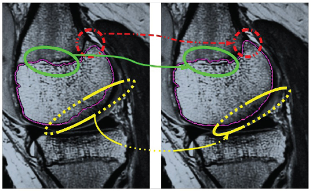
Segmentation by minimizing a meaningful image-dependent functional is not sufficient when the desired anatomic boundary is not actually a minimizer (left). By incorporating a control input to the gradient flow, sequential human inputs steer the dynamics so as to correctly segment the structure (right).

Direct labeling alone is unsatisfactory. First, there is no margin of error for careless mouse input from the user; great finesse is required. Second, simply switching between direct assignments of ϕ and evolution of the gradient flow ϕ_t = G(ϕ, I) will tend to override the user’s input during the automated phase. Rather than only directly affecting the state ϕ, input sent from the human expert can be incorporated into ϕ′s dynamics as a control input to ϕ_t.

If given infinite time, the human user would generate a particular ϕ(x, ∞). As the purpose of the proposed model is avoidance of tedious manual segmentation, it must be assumed that this quantity is not available. Rather, its estimate is denoted by ϕ*(x, t) and driven by a fast observer-like system that reacts to ϕ and the accumulated U:

$${\varphi }_t^{*}=F(\varphi ,{\varphi }^{*},U).$$ (7)

Incorporating both the nominal data-driven dynamics and influence of user inputs over time, the closed-loop system driving ϕ is

$${\varphi }_t=\underset{\text{nominal}}{\underbrace{G(\varphi ,I)}}+\underset{\text{control}}{\underbrace{H(\varphi ,{\varphi }^{*})}}.$$ (8)

Implementing the closed-loop dynamics of Section II-B requires particular choices for control signals F(ϕ, ϕ*, U) and H(ϕ, ϕ*) that should provide both stability and the desired dynamic response. Update laws for ϕ* and ϕ use the error signals

$$\widehat{\varphi }\doteq {\varphi }^{*}-\varphi ,e_U\doteq {\varphi }^{*}-U,$$ (9)

and are derived in Section III next.

III. Control Signal Design

We now synthesize control functions by establishing negative definiteness of several Lyapunov functions. This approach is motivated by existing literature in PDE systems. Boundary-control and stabilization of open-loop unstable systems [14]–[17] considers methods for establishing stability throughout a domain while actuating only a boundary. In contrast, precise actuation in the entirety of a domain is assumed in several methods for adaptive control under spatially varying uncertain functions [18], [19].

Image segmentation with PDEs requires a slightly different view of the actuation domain’s role. Both user input and ϕ(x, t) can be actuated anywhere in the domain, but the goal of reducing human effort motivates us to seek control strategies that minimize the domain in which U(x, t) is actuated. It is assumed that the user is satisfied with ϕ as an approximation for ϕ* when they are not generating input (|U| is small). In this case, ${\varphi }_t^{*}$ should cause ϕ* to follow ϕ. As U grows due to persistent human input, ϕ* becomes driven by U and ϕ by ϕ* instead of its nominal dynamics.

Proposition III.1 A control law for ϕ’s slow dynamics that drive it towards ϕ* can be found by augmenting the Lagrangian that led to ϕ_t = G(ϕ, I). Adding a penalty on $\frac{K_{\varphi }}{2}{\Vert \widehat{\varphi }\Vert }_{H^1}$ gives the functional

$$\mathscr{H}[\varphi ]={\int }_{\mathrm{\Omega }}\frac{K_{\varphi }}{2}({\widehat{\varphi }}^2+{\Vert \nabla \widehat{\varphi }\Vert }_2^2)+g(\varphi ,I){\Vert \nabla \varphi \Vert }_{2}d\mathrm{\Omega },$$ (10)

whose gradient flow smoothly blends the action of image-dependent potential g(ϕ, I) and estimate error ϕ. Corresponding to ℋ is the gradient flow

$${\varphi }_t=G(\varphi ,I)+K_{\varphi }(\widehat{\varphi }-\mathrm{\Delta }\widehat{\varphi }).$$ (11)

Furthermore, suppose that in the slow time-scale, the observer update signal ${\varphi }_t^{*}$ quickly settles to zero relative to ϕ̂. That is, for an ε > 0, 0 < $|{\varphi }_t^{*}|$ < ε|ϕ̂(ϕ̂ − Δϕ̂)| after some finite time t*. Then a sufficient condition for $\frac{d}{dt}\mathscr{H}[\varphi ]<0$ is K_ϕ > ε > 0.

Proof:

$$\frac{d}{dt}\mathscr{H}={\int }_{\mathrm{\Omega }}{K}_{\varphi }({\varphi }_t^{*}-{\varphi }_t)[\widehat{\varphi }-\mathrm{\Delta }\widehat{\varphi }]-{\varphi }_{t}G(\varphi ,I)d\mathrm{\Omega },$$ (12)

and for t > t*,

$$\frac{d}{dt}\mathscr{H}\le {\int }_{\mathrm{\Omega }}[-K_{\varphi }(\widehat{\varphi }-\mathrm{\Delta }\widehat{\varphi })-G(\varphi ,I)]{\varphi }_{t}d\mathrm{\Omega }+{\int }_{\mathrm{\Omega }}{K}_{\varphi }\epsilon ({\widehat{\varphi }}^2-\widehat{\varphi }\mathrm{\Delta }\widehat{\varphi })d\mathrm{\Omega }.$$ (13)

and the gradient flow for ϕ_t above is

$${\varphi }_t=G(\varphi ,I)+K_{\varphi }(\widehat{\varphi }-\mathrm{\Delta }\widehat{\varphi }).$$

The uncontrollable ${\varphi }_t^{*}$ term’s effect can be analyzed by substituting ϕ_t and integrating by parts, leading to the inequality

$$\frac{d}{dt}\mathscr{H}\le {\int }_{\mathrm{\Omega }}-{\varphi }_t^{2}d\mathrm{\Omega }+K_{\varphi }\epsilon {\Vert \widehat{\varphi }\Vert }_{H^1}^2\le {\int }_{\mathrm{\Omega }}-[[G^2+K_{\varphi }^2{(\widehat{\varphi }-\mathrm{\Delta }\widehat{\varphi })}^2]d\mathrm{\Omega }+K_{\varphi }\epsilon {\Vert \widehat{\varphi }\Vert }_{H^1}^2.$$ (14)

Expanding the (ϕ̂ − Δϕ̂)² term leads to

$$\frac{d}{dt}\mathscr{H}\le K_{\varphi }\epsilon {\Vert \widehat{\varphi }\Vert }_{H^1}^2+{\int }_{\mathrm{\Omega }}-[G^2+K_{\varphi }^2({\widehat{\varphi }}^2+2{\Vert \nabla \widehat{\varphi }\Vert }_2^2+{(\mathrm{\Delta }\widehat{\varphi })}^2]d\mathrm{\Omega },$$ (15)

giving a conservative sufficient condition for $\frac{d}{dt}\mathscr{H}\le 0$ of K_ϕ > ε > 0.

Proposition III.2 To obtain an update law for ϕ*’s fast dynamics, consider the functional

$$ℱ[{\varphi }^{*}]={\int }_{\mathrm{\Omega }}\frac{K_F}{2}{\widehat{\varphi }}^2+\frac{K_U}{2}{e}_U^2{(\gamma U)}^2+\frac{\mu }{2}({\varphi }^{*2}+{\Vert \nabla {\varphi }^{*}\Vert }_2^2)d\mathrm{\Omega }.$$ (16)

The first two terms above suggest that ϕ* will follow ϕ or U, depending on their relative magnitude. Regularization of ϕ* arises from the $\mu {\Vert {\varphi }^{*}\Vert }_{H^1}^2$ portion. A gradient flow that shrinks ℱ fastest is given by

$${\varphi }_t^{*}=[K_F\widehat{\varphi }+K_U{e}_U{(\gamma U)}^2+\mu ({\varphi }^{*}-\mathrm{\Delta }{\varphi }^{*})].$$ (17)

Proof: Define P(ϕ, ϕ*, Δϕ*, U) as the portion of the integrand’s derivative with a ${\varphi }_t^{*}$ factor:

$$P(·)\doteq K_F\widehat{\varphi }+K_U{e}_U{(\gamma U)}^2+\mu ({\varphi }^{*}-\mathrm{\Delta }{\varphi }^{*}).$$ (18)

The time derivative of functional Eq. 16 is then

$$\frac{d}{dt}ℱ={\int }_{\mathrm{\Omega }}{\varphi }_t^{*}P(·)d\mathrm{\Omega }-{\int }_{\mathrm{\Omega }}{\varphi }_t{K}_F\widehat{\varphi }d\mathrm{\Omega }.$$ (19)

The controllable term ${\int }_{\mathrm{\Omega }}{\varphi }_t^{*}P(·)d\mathrm{\Omega }$ shrinks fastest when ${\varphi }_t^{*}$ is proportional to −P(·) as proposed above in Eq. 17. However, it remains to establish that the integral term not controllable by ${\varphi }_t^{*}$ is stable.

Proposition III.3 Negativity $\frac{d}{dt}ℱ\le 0$ is guaranteed when

$$K_F{\Vert \widehat{\varphi }\Vert }_{L^2}>G_M|\mathrm{\Omega }|,$$

where G_M is a known pointwise bound on the nominal dynamics term and |Ω| is the domain’s Lebesgue measure.

Proof: Substituting ϕ_t = G(·) + K_ϕ(ϕ̂ − Δϕ̂), the second integral in $\frac{d}{dt}ℱ$ is

$$-{\int }_{\mathrm{\Omega }}{\varphi }_t{K}_F\widehat{\varphi }d\mathrm{\Omega }={\int }_{\mathrm{\Omega }}{K}_{\varphi }{K}_F(\widehat{\varphi }\mathrm{\Delta }\widehat{\varphi }-{\widehat{\varphi }}^2)-K_{\varphi }G\widehat{\varphi }d\mathrm{\Omega }.$$ (20)

From integration by parts,

$${\int }_{\mathrm{\Omega }}\widehat{\varphi }\mathrm{\Delta }\widehat{\varphi }d\mathrm{\Omega }=-{\int }_{\mathrm{\Omega }}\nabla \widehat{\varphi }·\nabla \widehat{\varphi }d\mathrm{\Omega }.$$

The uncontrolled integral Eq. 20 then is the negative H¹ Sobolev norm of ϕ̂ squared plus a term due to G:

$${\int }_{\mathrm{\Omega }}{\varphi }_t{K}_F\widehat{\varphi }d\mathrm{\Omega }=-{\Vert {(K_{\varphi }{K}_F)}^{\frac{1}{2}}\widehat{\varphi }\Vert }_{H^1}^2-{\int }_{\mathrm{\Omega }}G{K}_{\varphi }\widehat{\varphi }d\mathrm{\Omega }$$ (21)

$$=-K_{\varphi }{K}_F{\Vert \widehat{\varphi }\Vert }_{H^1}^2-{\langle G,K_{\varphi }\widehat{\varphi }\rangle }_{L^2},$$ (22)

which shall be abbreviated as Q(ϕ̂). Since the nominal dynamics G(ϕ, I) are known and arose from our choice of image-based cost function, it can be assumed that by construction |G| < G_M in the entire domain. Let |Ω| be the Lebesgue measure of domain Ω. From the Cauchy-Schwarz inequality, a conservative upper bound on Eq. 20 is given by

$$Q(\widehat{\varphi })\le -K_{\varphi }{K}_F{\Vert \widehat{\varphi }\Vert }_{H^1}^2+K_{\varphi }{\langle \widehat{\varphi },\widehat{\varphi }\rangle }_{L^2}^{1/2}{\langle G,G\rangle }_{L^2}^{1/2}$$ (23)

$$\frac{Q(\widehat{\varphi })}{K_{\varphi }}\le -K_{\varphi }{K}_F({\Vert \widehat{\varphi }\Vert }_{L^2}^2+{\Vert \nabla \widehat{\varphi }\Vert }_2^2)+K_{\varphi }{\Vert \widehat{\varphi }\Vert }_{L^2}{G}_M|\mathrm{\Omega }|.$$ (24)

Thus, we can guarantee the strict negativity

$$-{\int }_{\mathrm{\Omega }}{\varphi }_t{K}_{\varphi }\widehat{\varphi }d\mathrm{\Omega }\le 0$$ (25)

when ϕ-observer gain K_F is sufficently high as to make

$$K_F{\Vert \widehat{\varphi }\Vert }_{L^2}>G_M|\mathrm{\Omega }|.$$ (26)

Together with the update law ${\varphi }_t^{*}=-P(\cdot )$ of Eq. 17, satisfying the negativity condition of Eq. 25 renders the entire $\frac{d}{dt}ℱ\le 0$.

IV. Results

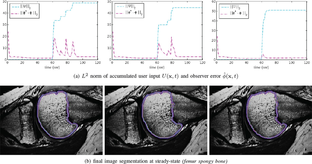
A numerical implementation of the gradient flow equations with user input from the preceding sections is used to segment an MRI dataset of a juvenile patient’s knee. First, as shown in Section IV, the final segmentations are consistent; this is vital if various clinicians are to use a fixed set of procedures with the software. Second, the system as whole indeed converges to a steady-state as predicted, and this steady-state ϕ(x, t) can be tuned with excellent precision by repeated user inputs.

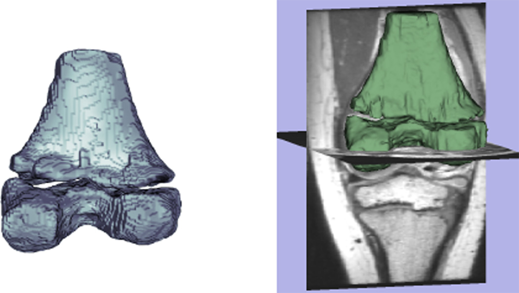
For this example, the dark patch on the cartilage-bone junction is where the nominal dynamics ϕ_t = G(ϕ, I) lead to an undesirable segmentation. After a brief period of user-input in painting this patch as inside, the steady-state shifts and captures this region. Notice that as the U reaches a final value (when the user stops editing), the observer error ‖ϕ̂‖_L² decreases to a steady state value corresponding to $\frac{d}{dt}ℱ=0$ from Theorem III.3. In this mode, the nominal dynamics and control of ϕ_t are balanced. In three dimensions, the example’s final output is shown in Fig. IV, having taken 8 minutes to run the system.

Fig. 4.

Explicitly modelling the visualization feedback to the user as a source of expert input provides insight into how to design both the automated portion of segmentation and the user interaction structure. Feedback compensates for deficiencies in automatic segmentation by exploiting the human expert’s interpretation of complex imagery.

V. Conclusions and Future Work

The preceding sections have presented an approach that connects interactive medical image segmentation and control-theoretic analysis and design. Using the implicit function and level set evolution approach, accumulated user inputs interact with both instantaneous state and dynamic response of the PDE system. Lyapunov control design enables a balance to be established between the influence of a data-driven gradient flow and the human’s input over time, with persistent input in a region of space leading to ϕ_t gradually deviating from its nominal gradient flow.

Control design in this paper has focused on the basic additive model ϕ_t = G(ϕ, I) + H(ϕ, ϕ*). As the inequalities of Section III are rather conservative, there is future work in determining more relaxed criteria. Given that even this simple additive model leads to some desirable closed-loop behavior, a more involved control strategy could potentially yield large improvements in interactive segmentation. Novel extensions include directly incorporating functions of the image data in control and determining optimal methods for providing display feedback to the user.

Fig. 5.

Timeline: after initialization, the inner loop of Section II updates ϕ and ϕ*. Input from a human user applies impulses at times t_k to ϕ and accumulates as U(x, t). Between times t_k, the inner loop changes steady-state in response to updated U(x, t). The user stops applying input when the visualization of ϕ(x, t) is satisfactory.

Fig. 6.

Consistent segmentations and convergent observer error are attained after user input stops.

Fig. 7.

Moving into 3D, a user’s time to segment high quality surfaces is cut dramatically over manual segmentation. Accuracy follows that of an underlying automatic method, except where user input as a correction has been applies.

Appendix

Image Processing with Gradient Flows

Preceding sections make use of integration by parts in ℝ^N several times, which we compactly review below in the context of differentiation of a functional. Γ is a piecewise smooth boundary, and Ω is a closed and bounded subset of ℝ^N. Integration by parts states that

$$\int \nabla \psi ·\mathbf{v}d\mathrm{\Omega }={\int }_{\mathrm{\Gamma }}(\psi \mathbf{v})·\widehat{N}d\mathrm{\Gamma }-{\int }_{\mathrm{\Omega }}\psi \nabla ·\mathbf{v}d\mathrm{\Omega },$$

To apply this to the derivative of a functional, let F(x, u(x, t), ∇u(x, t)) be a point-wise cost whose integral is to be minimized. The gradient here is with respect to spatial variables x. Computing the time-derivative,

$$\frac{d}{dt}ℱ[u(\mathbf{x},t)]=\frac{d}{dt}{\int }_{\mathrm{\Omega }}F(\mathbf{x},u,\nabla u)d\mathrm{\Omega }$$ (27)

$$={\int }_{\mathrm{\Omega }}[F_u{u}_t+F_{\mathbf{x}}\nabla u_t]d\mathrm{\Omega }.$$ (28)

Using the general form of integration by parts with v ≐ F_x and ψ ≐ u_t = 0 on the boundary Γ,

$$\frac{d}{dt}ℱ[u(\mathbf{x},t)]={\int }_{\mathrm{\Omega }}(F_u-\nabla ·F_{\mathbf{x}})u_{t}d\mathrm{\Omega }.$$ (29)

Applying Cauchy-Schwarz in L²,

$$|\langle u_t,F_u-\nabla ·F_{\mathbf{x}}\rangle |\le \Vert F_u-\nabla ·F_{\mathbf{x}}\Vert \Vert u_t\Vert ,$$

so that a gradient flow direction for u(x, t) is

$$u_t=-C\frac{F_u-\nabla ·F_{\mathbf{x}}}{{\Vert F_u-\nabla ·F_{\mathbf{x}}\Vert }_{L^2}},C>0\text{constant}.$$ (30)

References

- 1.Balafar M, Ramli A, Saripan M, Mashohor S. Review of brain MRI image segmentation methods. Artificial Intelligence Review. 2010;vol. 33(no. 3):261–274. [Google Scholar]
- 2.Petitjean C, Dacher J. A review of segmentation methods in short axis cardiac MR images. Medical Image Analysis. 2010:1. doi: 10.1016/j.media.2010.12.004. [DOI] [PubMed] [Google Scholar]
- 3.De Boer R, Vrooman H, Ikram M, Vernooij M, Breteler M, Van der Lugt A, Niessen W. Accuracy and reproducibility study of automatic MRI brain tissue segmentation methods. NeuroImage. 2010;vol. 51(no. 3):1047–1056. doi: 10.1016/j.neuroimage.2010.03.012. [DOI] [PubMed] [Google Scholar]
- 4.Chan T, Vese L. Active contours without edges. IEEE Transactions on image processing. 2001;vol. 10(no. 2):266–277. doi: 10.1109/83.902291. [DOI] [PubMed] [Google Scholar]
- 5.Michailovich O, Rathi Y, Tannenbaum A. Image segmentation using active contours driven by the bhattacharyya gradient flow. IEEE Transactions on Image Processing. 2007;vol. 16(no. 11):2787–2801. doi: 10.1109/tip.2007.908073. [DOI] [PMC free article] [PubMed] [Google Scholar]
- 6.Platero C, Tobar M, Sanguino J, Poncela J. Appearance and shape prior alignments in Level Set Segmentation. Pattern Recognition and Image Analysis. 2009:282–289. [Google Scholar]
- 7.El-Baz A, Gimelfarb G. Robust Medical Images Segmentation Using Learned Shape and Appearance Models. Medical Image Computing and Computer-Assisted Intervention–MICCAI 2009. 2009:281–288. doi: 10.1007/978-3-642-04268-3_35. [DOI] [PubMed] [Google Scholar]
- 8.Essafi S, Langs G, Paragios N. Computer Vision and Pattern Recognition, 2008. CVPR 2008. IEEE Conference on. IEEE; 2008. Sparsity, redundancy and optimal image support towards knowledge-based segmentation; pp. 1–7. [Google Scholar]
- 9.Pieper S, Lorensen B, Schroeder W, Kikinis R. The namic kit: Itk, vtk, pipelines, grids and 3d slicer as an open platform for the medical image computing community. Biomedical Imaging: Nano to Macro, 2006. 3rd IEEE International Symposium on. IEEE. 2006:698–701. [Google Scholar]
- 10.Pieper S, Halle M, Kikinis R. 3D Slicer. Biomedical Imaging: Nano to Macro, 2004. IEEE International Symposium on. IEEE. 2005:632–635. [Google Scholar]
- 11.Seg3D: Volumetric Image Segmentation and Visualization. Scientific Computing and Imaging Institute (SCI); [Online]. Available: http://www.seg3d.org. [Google Scholar]
- 12.Sethian J. Level set methods and fast marching methods: evolving interfaces in computational geometry, fluid mechanics, computer vision, and materials science. Cambridge University Press; 2000. [Google Scholar]
- 13.Osher S. Level set methods. Geometric Level Set Methods in Imaging, Vision, and Graphics. 2003:3–20. [Google Scholar]
- 14.Krstic M, Smyshlyaev A. Backstepping boundary control for first-order hyperbolic PDEs and application to systems with actuator and sensor delays. Systems & Control Letters. 2008;vol. 57(no. 9):750–758. [Google Scholar]
- 15.Krstic M, Guo B, Balogh A, Smyshlyaev A. Output-feedback stabilization of an unstable wave equation. Automatica. 2008;vol. 44(no. 1):63–74. [Google Scholar]
- 16.Krstic M, Smyshlyaev A. Society for Industrial Mathematics. Boundary control of PDEs: A course on backstepping designs. 2008 [Google Scholar]
- 17.Krstic M, Magnis L, Vazquez R. Nonlinear control of the viscous Burgers equation: Trajectory generation, tracking, and observer design. Journal of Dynamic Systems, Measurement, and Control. 2009;vol. 131:021012. [Google Scholar]
- 18.Kim J, Bentsman J. Robust model reference adaptive control of parabolic and hyperbolic systems with spatially-varying parameters. Decision and Control, 2005 and 2005 European Control Conference. CDC-ECC’05. 44th IEEE Conference on. IEEE. 2005:1503–1508. [Google Scholar]
- 19.Kim J, Bentsman J. Disturbance rejection in robust model reference adaptive control of parabolic and hyperbolic systems. Decision and Control, 2006 45th IEEE Conference on. IEEE. 2006:3083–3088. [Google Scholar]