Binding Interface Prediction by Combining Protein-protein Docking Results

Abstract

We developed a method called Residue Contact Frequency (RCF), which uses the complex structures generated by the protein-protein docking algorithm ZDOCK to predict interface residues. Unlike interface prediction algorithms that are based on monomers alone, RCF is binding partner specific. We evaluated the performance of RCF using the Area Under the Precision-Recall (PR) Curve (AUC) on a large protein docking Benchmark. RCF (AUC=0.44) performed as well as meta-PPISP (AUC=0.43), which is one of the best monomer-based interface prediction methods. In addition, we test a Support Vector Machine (SVM) to combine RCF with meta-PPISP and another monomer-based interface prediction algorithm Evolutionary Trace to further improve the performance. We found that the SVM that combined RCF and meta-PPISP achieved the best performance (AUC=0.47).

We used RCF to predict the binding interfaces of proteins that can bind to multiple partners and RCF was able to correctly predict interface residues that are unique for the respective binding partners. Furthermore, we found that residues that contributed greatly to binding affinity (hotspot residues) had significantly higher RCF than other residues.

Introduction

Protein-protein interactions control biological processes such as signaling transduction, immune responses and enzymatic activities. It is of great interest to understand how proteins interact with one another and the knowledge can aid the search for therapeutic targets. High-throughput experiments such as yeast-two-hybrid and mass spectrometry can identify interacting proteins;^1,2 however, these techniques do not elucidate the binding mode or the binding interface. Other experimental procedures such as mutagenesis (especially alanine scan) can identify residues that play a key role in the interaction. X-ray crystallography and nucleic magnetic resonance (NMR) can solve the atomic structure of a protein-protein complex. Nonetheless, solving protein complex structures remains challenging, especially for weakly interacting proteins, which are hard to capture in the complexed form. Computational algorithms for predicting complex structures or binding sites can complement the experimental procedures.

The properties of protein-protein binding interfaces have been studied extensively. Jones and Thornton showed that solvation potential, residue interface propensity, hydrophobicity, planarity, protrusion and accessible surface area had the potential to distinguish binding interface from the rest of protein surface.³ The interface tends to be more hydrophobic⁴ and more planar,⁵ and contains a core with distinct amino acid composition compared with the rest of the protein surface.⁶ Such findings have been used to develop algorithms for interface prediction. The ProMate algorithm uses protein secondary structure composition, clusters of polar and hydrophobic residues, locations of crystal water molecules and B-factor data.⁷ The PINUP algorithm uses side chain energy, residue interface propensity and sequence conservation.⁸ The cons-PPISP algorithm uses sequence profiles and solvent accessibility of neighboring residues.⁹ meta-PPISP is a meta-server that integrates the outputs of PROMATE, cons-PPISP and PINUP.¹⁰ CPORT¹¹ is also a consensus method combining interface predictions from WHISCY¹², PIER¹³, ProMate, cons-PPISP, SPPIDER¹⁴ and PINUP. All these algorithms use protein monomers as input and do not explicitly consider the properties of their binding partners.

Most proteins interact with multiple other proteins,¹⁵ some involving unique interfaces. Thus monomer-based interface prediction algorithms are inherently limited, as they cannot predict interfaces specific to different binding partners. Docking algorithms such as ZDOCK¹⁶ predict the atomic structures of protein-protein complexes, thus can predict the binding interfaces in a binding partner specific way. Nonetheless, docking algorithms often generate predictions that differ to various extents from the correct binding mode. Fernandez-Recio presented the NIP method, which used a collection of docking predictions to derive a consensus of predicted interface residues.¹⁷ We introduced Atom Contact Frequency (ACF),¹⁸ which uses the consensus of ZDOCK predictions to predict interface residues. Bonvin and colleagues used the monomer-based interface prediction method CPORT to drive their docking algorithm and then used the docking results to make another round of interface prediction. They showed that the second round of interface predictions made using the collection of docking results improved upon the initial set of CPORT predictions.¹¹

In this work we introduce the binding partner-specific interface prediction algorithm Residue Contact Frequency (RCF), which was derived from ACF, as well as the combination of RCF with monomer-based interface prediction methods through a Support Vector Machine (SVM). Specifically, we test terms from the algorithms Evolutionary Trace (ET) and meta-PPISP¹⁰. ET constructs a multiple sequence alignment to compute sequence conservation, and was used as a feature of an SVM for protein interface prediction.¹⁹ meta-PPISP¹⁰ is a meta server that incorporates predictions from PROMATE, cons-PPISP and PINUP. Our combined method improves upon RCF alone and outperforms the monomer-based interface prediction algorithms. We also applied RCF to proteins with multiple binding partners and showed that it accurately predicted binding partner-specific interface residues.

Protein-protein interactions are often governed by a limited number of amino acids in the binding interface that have relatively high energetic contributions to the interaction,²⁰ and these residues are commonly referred to as hotspots residues. Alanine scanning is the standard experimental technique for identifying hotspots residues. We also used RCF to predict hotspot residues from unbound structures.

There are many ways that our RCF algorithm can be used in practice. For example, mutagenesis experiments can be steered by the RCF interface prediction, which is supported by the correlation between RCF and hotspot residues. Also, docking algorithms can be guided using predicted interface residues, as shown by Bonvin and colleagues.¹¹ Finally, our findings on binding-partner specificity of interface residues can eventually be incorporated in structural analysis of protein-protein interaction networks.

Materials and Methods

Datasets

We used the protein-protein docking benchmark (version 4.0)²¹ for training and testing our methods. We excluded 14 structures because meta-PPISP (unbound PDB IDs: 1CJE, 1CZP, 3MIN, 2GHU, 2H7O) or ET (unbound PDB IDs: 3GMU, 1MKF, 1NYC, 2UGI, 1XK9, 1ZFI, 2H70, 2UUX, 1H20) failed to generate output files (possibly due to the lack of homologous sequences). In addition, antibody-antigen test cases were excluded. The antigen-binding interface of an antibody comprises hypervariable loops derived from combinatorial assembly of genomic segments and untemplated addition of nucleotides, and it is not evolutionarily conserved. Because meta-PPISP uses sequence conservation and ET uses evolutionary pressure, these methods are not suitable for the prediction of antibody-antigen interfaces. The resulting data set contained 286 monomers and 143 complexes.

An interface residue must have at least one atom within 6 Å of any atom of the binding partner and at least 5% relative solvent accessible surface area (compared with the average area of that residue type). We used the NACCESS algorithm²² to calculate solvent accessibility.

For analyzing hotspot residues, we used the alanine scan data from SKEMPI.²³ There are 3047 ΔΔG measurements from 158 protein structures in SKEMPI. We used the alanine scanning ΔΔG measurements of 253 interface residues from the 32 protein structures that coexist in SKEMPI and Benchmark4.0. Hotspot residues are defined as ΔΔG ≥ 2 kcal/mol.

Individual interface prediction methods

Residue Contact Frequency (RCF)

Previously we introduced the Atom Contact Frequency (ACF),¹⁸ which reflects how often an atom is present in the binding interface in a set of predicted protein-protein complex structures. We define the Atom Contact Frequency (N_i) for the i-th atom as the number of contacts (n_ik) this atom makes with any atom of the k-th predicted orientation of the binding partner. We used a 6 Å cutoff for defining a contact, and normalized the result:

$$N_i=M_i/max\{M_1,\cdots ,M_j,\cdots \},\text{where}{M}_i=\sum _k{n}_{ik}$$ (1)

In our previous work, we predicted a residue to be in the interface if it has any atom with ACF ≥ 0.7. In this study, we calculated the RCF R_x for a residue x by summing the ACFs of all atoms that belong to residue x. RCF and ACF performed similarly for interface residue prediction (Supporting Information Figure S1), but RCF was better able than ACF in the differentiation of hotspot residues from non-hotspot residues (Kolmogorov-Smirnov test for testing the hotspot distribution vs. the non-hotspot distribution resulted in p-values of 9.1×10⁻⁵ for RCF and 3.6×10⁻³ for ACF). Therefore we use RCF for the results presented in this work.

We used ZDOCK to generate the collection of predicted complex structures that ACF and RCF are calculated from. We used a 15° angular sampling, which results in 3600 predictions for each test case. ZDOCK predictions are ranked based on ZDOCK score. We tested the performance of RCF and ACF with a range of rank cutoffs (i.e., k=1, 2, …, K in equation 1, with K = 10, 100, 1000, 2000, 3000, 3600) and found the best RCF performance with K = 2000 (Supporting Information Figure S1). This figure indicates that the consensus approach of ACF and RCF (Area Under the precision and recall Curve (AUC) ≥ 0.437) performs better than using all 3600 predictions (AUC=0.410).

The code for computing the RCF values is available over the Internet: zlab.umassmed.edu/RCF/

Evolutionary Trace and meta-PPISP

the ET score for each residue²⁴ was obtained from the ET server (http://mammoth.bcm.tmc.edu/ETserver.html). A larger ET score indicates weak sequence conservation, and it is known that interface residues are generally more conserved than other surface residues.¹⁹ Because also buried residues are generally more conserved but are unlikely to be in the interface, we assigned the maximum ET score observed anywhere in the protein to the residues that are buried (relative solvent accessible surface area < 5%). meta-PPISP¹⁰ scores were obtained from a web server (http://pipe.scs.fsu.edu/meta-ppisp.html). Note that both meta-PPISP and RCF have their own definition of surface residues,¹⁰ but since 97.1% of the RCF defined surface residues are also defined as surface residues by meta-PPISP, we consider the two definitions to be compatible.

SVM and performance evaluation

We used LIBSVM with the linear kernel²⁵ for constructing an SVM. All the results presented here were obtained using leave-one-out cross-validation. We used Precision-Recall (PR) curves and the associated Area Under the Curve (AUC) for evaluation the performance of each method. Precision and Recall were defined as:

$$\begin{array}{l}\text{Precision}=\text{TP}/(\text{TP}+\text{FP})\\ \text{Recall}=\text{TP}/(\text{TP}+\text{FN})\end{array}$$ (2)

where true positives (TP) denotes the number of correctly predicted interface residues, false positives (FP) denotes the number of residues incorrectly predicted to be in the interface, and false negatives (FN) denotes the number of residues incorrectly predicted not to be in the interface. The PR curve corresponding to random predictions is a flat line with precision equal to the ratio of interface residues to the number of total residues, and the AUC of PR curve of random predictions is equal to this ratio as well. In the sections below we display PR curves of random predictions along with RCF PR curves, and we use the AUC of the PR curve of random predictions to assess whether RCF results are better than random.

Results and Discussion

Comparison of individual interface prediction methods

We first evaluated the performance of RCF, ET, and meta-PPISP individually.²⁶ Figure 1A shows that RCF and meta-PPISP perform similarly (with AUC = 0.44 and 0.43, respectively). ET performs worse (AUC = 0.29), yet better than what is expected by chance (AUC = 0.20). Table I shows the correlation among the three methods, calculated using all test cases. Although RCF and meta-PPISP have similar predictive power, their scores are only moderately correlated (r = 0.46), suggesting that ACF and meta-PPISP can complement each other in a SVM.

Figure 1.

PR curves for individual methods and for different categories of test cases. Dotted lines are expected PR curves for random predictions.

Table I.

Correlation coefficient r among the scores computed by the three methods.

	ETa	RCF
meta-PPISP	−0.34	0.46
ETa		−0.20

^aET stands for Evolutionary Trace

We further compared the performance of RCF and the performance of ZDOCK, of which the predictions were used to generate the RCF results. We first compared the interface predicted by RCF with the interface of the top-ranked ZDOCK prediction (ZDOCK1). We asked RCF to predict the same number of interface residues as in the ZDOCK1 interface. We computed precision for each method, defined as the number of correctly predicted interface residues divided by the number of predicted residues. Figure 2 shows the RCF precision against the ZDOCK1 precision for each protein in the benchmark. Out of the 286 proteins in our test set, RCF was better than ZDOCK1 for 148 proteins (points above the diagonal), RCF was worse than ZDOCK1 for 119 proteins (points below the diagonal), and the two methods tied for the remaining 19 proteins (points on the diagonal). The differences correspond to a one-tailed p-value of 0.033 using the sign test. This shows that on average RCF performed better for interface residue prediction than the top-ranked ZDOCK prediction, which is consistent with our observation from Figure S1 that RCF achieved its best performance using the top 2000 ZDOCK predictions. Interestingly, there were 30 proteins for which ZDOCK1 precisions were zero, but RCF achieved higher precisions (highlighted in the circles marked 1 and 2). For these proteins, even though the ZDOCK1 interface shared no residue with the native interface, the integrated approach of RCF was still able to make meaningful predictions.

Figure 2.

Interface residue prediction precisions of RCF against the top-ranked ZDOCK prediction. The 286 proteins are classified into three categories: proteins for which the top-ranked ZDOCK prediction is a hit (ZDOCK 1st hit); proteins for which ZDOCK failed to generate a hit in top 2000 predictions (ZDOCK no hit 2000); proteins for which ZDOCK generated at least one hit with a rank between 2 and 2000 (Others). Indicated in the circles are: 1,2) proteins for which RCF and the top-ranked ZDOCK prediction have non-zero and zero precision, respectively; 2,3,4) ligands of test cases 1F34, 2OOB, and 1PXV, respectively.

Furthermore, we divided the proteins of the benchmark into three groups, indicated by different colors in Figure 2. Blue diamonds correspond to the group for which ZDOCK1 is a hit (defined as having interface RMSD from the native structure less than 2.5Å). We see that all the points are on or below the diagonal, which indicates that a high-quality ZDOCK1 structure always predicted the interface better than or the same as RCF. The other two groups are the proteins for which at least one of the top 2000 ZDOCK predictions (the number of predictions used for RCF) was a hit (green triangles), and the proteins for which ZDOCK did not have any hits in the top 2000 predictions (maroon squares). We see that even when ZDOCK did not produce any hits within the top 2000 predictions, RCF could still perform well for some of the proteins. We also observed that the RCF values of the group with a hit in the top 2000 (but not at rank 1) and the group with no hits in the top 2000, have different distributions (p-value 0.004 using the Kolmogorov-Smirnov test), with average RCF values of 0.42 and 0.33, respectively. This again demonstrates that the performances of ZDOCK and RCF are related.

We will now discuss in detail several proteins indicated in Figure 2. Circled and marked 2 is Ascaris pepsin inhibitor-3, which binds to porcine pepsin (PDB 1F34). ZDOCK1 was not a hit (interface RMSD = 24.5 Å); the first ZDOCK hit was ranked 68. Even though none of the 41 interface residues of ZDOCK1 overlapped with the native interface residues, 27 out of 41 interface residue predicted by RCF overlapped with the native interface residues. Thus RCF performs much better than ZDOCK1 for this case. Interestingly, of the 14 interface residues incorrectly predicted by RCF, seven overlapped with the interface residues of ZDOCK1. Thus RCF and ZDOCK1 did bear some resemblance, but the integration by RCF clearly moved away from the wrong ZDOCK1 prediction.

The proteins circled and marked 3 and 4 in figure 2 are also revealing. Both ZDOCK1 and RCF achieved high precisions (0.78 to 0.96) for the ligands of test cases 2OOB (marked 3) and 1PXV (marked 4). Surprisingly, for both test cases there was not a hit in the 2000 top-ranked ZDOCK predictions. This can be explained by also considering the receptors of both cases: the precisions of ZDOCK1 and RCF ranged from 0.21 to 0.45 (in both cases, the RCF precision was higher than the ZDOCK1 precision). Thus ZDOCK predicted the correct interface residues for the ligands, but paired them with the wrong residues of the receptor: The interface RMSDs for the top-ranked ZDOCK predictions of 2OOB and 1PXV were 9.85 and 13.25 Å respectively. Thus even when ZDOCK predicts the wrong binding mode, it can still predict the interface of one binding partner correctly and these correct predictions are preserved by RCF.

Next we investigated the performance for the different categories of test cases in the benchmark, classified according to biological function (enzyme-inhibitor and others) or expected docking difficulty (rigid-body, medium-difficulty, and difficult). The fractions of interface residues differ slightly among the categories, reflected in the PR curves of random predictions. Panels B, C and D of Figure 1 show the performance for the different categories of expected docking difficulty. Both RCF and meta-PPISP performed better for the rigid-body category (AUC = 0.46 for both) than for the medium-difficulty category (AUC of RCF = 0.41 and AUC of meta-PPISP = 0.39) and the difficult category (AUC of RCF = 0.39 and AUC of meta-PPISP = 0.37).

It is expected that RCF performs the best on rigid-body test cases, as RCF is computed from the predictions of the rigid-body docking algorithm ZDOCK, which is known to be the most reliable for test cases that show little conformational changes upon binding. Nonetheless, RCF derives a consensus from the top 2000 ZDOCK predictions, thus RCF can correctly predict the interface even if ZDOCK does not accurately predict the binding mode. For example, the bound and unbound structures of the receptor of the ‘difficult’ test case 1PXV differ by a root mean square deviation (RMSD) of 3.6 Å and the top 2000 ZDOCK predictions do not include any predictions with RMSD ≤ 2.5 Å from the crystal structure of the complex. The AUC of RCF is 0.76 (compared with AUC = 0.43 for random predictions), indicating that for this case RCF is able to predict the interface with good accuracy, leveraging multiple ZDOCK predictions that are close to the correct binding mode.

Meta-PPISP performs better for the rigid-body category than for the medium-difficulty and difficult categories, although it is a monomer-based method and should not be affected by docking difficulty. This may be due to the impact of binding affinity. Enzyme-inhibitor complexes often bind strongly, and both docking-based and monomer-based approaches should capture this to some extent. The correlation of the AUC with the binding free energy, calculated using the 107 cases shared between the docking Benchmark and the Affinity Benchmark²⁷, is not significant (r = 0.15 and 0.13 for RCF and meta-PPISP, with p-values of 0.12 and 0.11, respectively), which indicates that a simple analysis is not sufficient for explaining this effect. The best performance of ET was found for the medium-difficulty test cases (AUC = 0.32), followed by rigid-body test cases (AUC = 0.29) and difficult test cases (AUC = 0.26); however the differences are small.

Panels E, F and G of Figure 1 show that all three methods performed better for enzyme-inhibitor test cases than for other test cases. Again, reasons may be that active sites of enzymes are highly conserved (meta-PPISP and ET)²⁸ enzyme-inhibitor complexes have good shape complementarity (RCF),²⁹ and training was performed on enzyme-inhibitor complexes (meta-PPISP).

An SVM that combines RCF, meta-PPISP and ET

We used an SVM to combine RCF with meta-PPISP and additionally with ET. Figure 3A shows that the SVM that combines RCF with meta-PPISP performed better (AUC = 0.47) than the individual methods (AUC = 0.29–0.44). We include RCF (AUC = 0.44) in Figure 3A for comparison. The improvement obtained from adding ET was small (AUC = 0.48), thus we decided to exclude ET in the final SVM.

Figure 3.

PR curves for SVMs and RCF, and for different complex categories. In panel A, SVM (RCF + meta-PPISP) stands for the SVM with RCF and meta-PPISP only, and SVM (RCF + meta-PPISP + ET) stands for the SVM that combines all three methods.

Panels B and C of Figure 3 show the performance of the final SVM for the different categories of test cases. Like the individual methods, SVM performed better for enzyme-inhibitor test cases (AUC=0.58) than for other test cases (AUC=0.43, Figure 3B). The performance of the SVM on categories based on expected docking difficulty also follows the same trend as the individual methods, with the best performance for the rigid-body category and the worst performance for the difficult category (Figure 3C). SVM performed better than any of the individual methods for all the categories (compare Figure 3BC with Figure 1). This indicates that the success of the SVM approach is not limited to any particular category of test cases. The proteins in our Benchmark have on average 30 interface residues. For this number of predicted interface residues, the precision of the SVM is 0.52 and the recall is 0.45.

We compared our approach with the NIP method developed by Fernandez-Recio et al.¹⁷ which also uses docking results to predict interface residues. The test set used by Fernandez-Recio and our benchmark had 12 cases in common, thus we had 24 proteins to compare. For each of these proteins we compared the NIP precision and recall values from ref.³⁰ with the RCF PR curve for the same protein. When the NIP precision-recall point was below the RCF PR curve, it indicated that RCF performed better than NIP and vice versa. Comparing RCF with NIP, we found RCF performed better for 11 proteins, NIP performed better for 9 proteins, and the two methods tied for the remaining 4 proteins. Figure S2 shows the average NIP PR values and the average RCF PR curve over all 24 monomers. Thus RCF outperforms NIP on average. When we combined RCF and meta-PPISP in an SVM, we found that the SVM performed better than NIP for 13 proteins while NIP perform better for 6 proteins (one protein was excluded as the meta-PPISP calculation failed, and the SVM and NIP tied for the remaining four proteins), which shows that combining monomer-based and binding partner specific approaches indeed improves performance over either method by itself.

Binding partner-specific interface prediction

Many proteins have multiple binding partners and the binding interfaces for the different partners may be unique or only partially shared.^31,32 We investigated the ability of RCF to identify interface residues specific to each binding partner. Although the SVM performs better than RCF for interface residue prediction in general (as showed in Figure 3), we use only the RCF score here, as it is the only component of the SVM that can make binding partner-specific predictions.

The docking benchmark includes ten proteins that have multiple binding partners. For any two binding partner of a protein, we define unique interface fraction for each partner as the number of interface residues that are unique for this partner divided by the total number of interface residues for this partner, using the crystal structures of the two complexes. Thus unique interface fractions range between 0 and 1, with 0 indicating that no interface residue is unique for that partner, and 1 indicating that all the interface residues are unique for that partner.

Take the A1 domain of von Willebrand factor (vWF A1) as an example. vWF A1 forms a complex with bortrocetin (complex PDB ID: 1IJK)³³ and forms a complex with glycoprotein Ib-α (PDB ID: 1M10).³⁴ vWF A1 has 21 and 34 interface residues in the complexes with bortrocetin and glycoprotein Ib-α, respectively, of which 3 residues are shared. Thus the unique interface fractions for bortrocetin and glycoprotein Ib-α are 0.86 and 0.91 respectively. We used RCF to predict the interface residues of vWF A1 for these two partners. With respect to bortrocetin, the AUC of RCF is 0.24 for the entire interface (21 residues) and 0.50 for the 18 bortrocetin-specific residues, compared with random AUC of 0.10 and 0.09 respectively. Likewise for glycoprotein Ib-α, the AUC of RCF is 0.61 for the entire interface (34 residues) and 0.54 for the 31 glycoprotein Ib-α-specific residues, compared with random AUC of 0.16 and 0.15 respectively.

When a protein has more than two binding partners, we calculated unique interface fractions in a pair-wise fashion and averaged them and likewise, we computed the AUCs for partner-specific interface residues in a pair-wise manner and averaged them. Table II summarizes the results for the binding partner-specific interface prediction. The unique interface fractions show that for most proteins the interfaces are at least 1/3 unique. The average AUC for predicting the entire interface is 0.55, compared with the average AUC of 0.17 for random predictions (p-value = 2.6 × 10⁻⁵ for the entire set of interfaces in Table II, computed using paired Wilcoxon rank sum test). For only two out of the ten proteins (tissue factor and complement C3) and the complex of hen lysozyme with one partner, the performance of RCF for predicting the entire interface was no better than random predictions. The performance of RCF for predicting partner-specific interface residues was inferior to the performance for predicting the entire interface, yet significantly better than random predictions— average AUC for RCF is 0.25 compared with AUC of 0.10 for random predictions (p-value = 4.6 × 10⁻⁵ for the entire set of interfaces in Table II, computed using paired Wilcoxon rank sum test). In addition to the proteins for which RCF failed to predict the entire interfaces, ubiquitin posed a difficult case for partner-specific interface residue prediction. Overall, RCF is able to make predictions better than random for 20 out of 26 complexes.

Table II.

Binding partner-specific interface prediction using RCF

Unbound PDB	Bound PDB_chain	Unique interface fraction (σ)	AUCa for the entire interface	Random prediction for the entire interface	AUCa for partner-specific interface residues (σ)	Random predictio n for partner-specific interface residues
1QG4 (Ran GTPase)	1A2K_C	0.53	0.75	0.08	0.54	0.05
	1I2M_A	0.72	0.61	0.14	0.58	0.10
1AUQ (von Willebrand Factor A1)	1IJK_A	0.86	0.24	0.10	0.50	0.09
	1M10_A	0.91	0.61	0.16	0.54	0.15
2CGA (Chymotrypsin)	1ACB_E	0.00	0.59	0.09	NA	NA
	1CGI_E	0.28	0.74	0.13	0.14	0.04
1JAE (α-amylase)	1CLV_A	0.35	0.68	0.09	0.09	0.03
	1TMQ_A	0.35	0.77	0.09	0.12	0.03
1TFH (Tissue factor)	1AHW_C	0.16	0.15	0.22	0.02	0.19
	1JPS_T	0.13	0.11	0.15	0.01	0.12
1C3D (Complement C3)	1GHQ_A	1.00	0.03	0.05	0.03	0.05
	3D5S_A	1.00	0.11	0.09	0.12	0.09
1IJJ (Actin)	1KXP_A	0.64	0.51	0.11	0.23	0.07
	2BTF_A	0.46	0.62	0.07	0.22	0.03
1YJ1 (Ubiquitin)	1S1Q_B	0.35 (0.076)	0.83	0.52	0.19(0.052)	0.19
	1XD3_B	0.41 (0.018)	0.82	0.54	0.20(0.031)	0.22
	2OOB_B	0.09 (0.078)	0.89	0.39	0.07(0.011)	0.04
3LZT (Hen lysozyme)	1BVK_F	0.82 (0.175)	0.53	0.16	0.41(0.117)	0.13
	1DQJ_C	0.72 (0.288)	0.35	0.20	0.27(0.073)	0.14
	1MLC_E	0.83 (0.288)	0.11	0.14	0.12(0.038)	0.12
	2I25_L	0.85 (0.090)	0.80	0.47	0.66(0.103)	0.40
1MH1 (Rac GTPase)	1E96_A	0.81 (0.084)	0.32	0.10	0.42(0.096)	0.08
	1HE1_C	0.55 (0.191)	0.64	0.14	0.21(0.034)	0.08
	1I4D_D	0.47 (0.256)	0.92	0.11	0.31(0.245)	0.05
	2FJU_B	0.37 (0.244)	0.74	0.07	0.18(0.239)	0.03
	2H7V_A	0.43 (0.299)	0.67	0.11	0.22(0.051)	0.05
	2NZ8_A	0.48 (0.208)	0.73	0.14	0.14(0.033)	0.07

^aAUC stands for Area Under the Precision-Recall Curve

(σ) Standard deviations are provided in parentheses for proteins with more than two binding partners.

A Case study with Ran GTPase

Ran GTPase from the Ras-family is one of the key proteins in nucleocytoplasmic transport, and it forms complexes with Regulator of Chromosome Condensation 1 (RCC1)³⁵ and Nuclear transport factor 2 (NTF2)³⁶. RCC1 is the guanine nucleotide exchange factor for Ran GTPase³⁵ and NTF2 binds to Ran GTPase for efficient nuclear protein import.³⁶ Here we examine in detail the binding partner-specific interface prediction for Ran GTPase.

Ran GTPase has 8 residues in common between the interface with RCC1 and the interface with NTF2, thus the unique interface fractions are 0.72 and 0.53 for binding with RCC1 and NTF2, respectively. Figure 4 shows the RCF results for these two complexes. Panels A and B show the PR curves evaluated with all interface residues as well as with the residues specific to each binding partner, which show much higher AUCs than the PR curves that correspond to random predictions. Panels C and D overlay RCF scores on surface residues of Ran GTPase (higher RCF scores correspond to hotter colors) with respect to each of the binding partners. When Ran GTPase was paired with NTF2, Y39 and Y72 had the highest RCF scores, and these two residues are indeed in the center of the interface with NTF2. Likewise, when RCC1 was paired with Ran GTPase, K99 and F138 had the highest RCF scores and these two residues are in the interface with RCC1. Thus RCF correctly predicted the interface residues specific to each binding partner.

Figure 4.

Panels A and B: Ran GTPase PR curves with the entire interface (black) and only the partner-specific interface residues (grey). Also shown are the PR curves that correspond to random predictions. Panels C and D: Visual representation of RCF values in color (redder for higher RCF) for Ran GTPase with NTF2 (C) and RCC1 (D) as the binding partner (shown in wheat).

ΔΔG prediction using unbound protein structures

Previously we reported that residues with high ACF tended to be located near the centers of the protein-protein interfaces.¹⁸ Because hotspot residues are often found in the center of interfaces,²⁰ we tested whether RCF could discriminate hotspot residues (defined by ΔΔG ≥ 2 kcal/mol with alanine scanning²⁰) from non-hotspot residues (ΔΔG < 2 kcal/mol). Because RCF is calculated using the unbound-unbound docking results of ZDOCK, we do not need to know the structure of the complex. We used the SKEMPI database, which is a compilation of experimentally measured ΔΔG values.³⁷ We only used the complexes that were present in both SKEMPI and Benchmark 4.0, resulting in 253 residues (71 hotspots and 182 non-hotspot residues) from the interfaces of 21 complexes. Figure 5 shows that the RCF scores of hotspot interface residues are significantly higher than those of non-hotspot residues (p-value = 9.1×10⁻⁵ using the Kolmogorov-Smirnov test), which indicates that the RCF approach can be used for predicting alanine scanning data.

Figure 5.

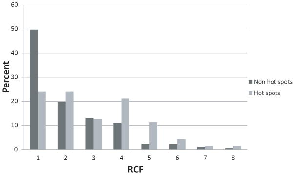
Distribution of RCF scores for hotspot residues and non-hotspot residues. The distributions are significantly different (p-value = 9.1×10⁻⁵using the Kolmogorov-Smirnov test).

Conclusion

We reported a protein-protein interface prediction method, RCF, which is binding partner specific because it is computed using protein-protein docking results. In addition, we tested a support vector machine to combine RCF with the monomer-based interface prediction methods meta-PPISP and Evolutionary Trace, found that adding meta-PPISP improved upon RCF alone, but further addition of Evolutionary Trace did not. We showed that RCF outperforms the monomer-based approaches, and that the integration using the SVM yields the best performing approach. The docking Benchmark includes ten proteins with multiple binding partners, and we showed that RCF can be used to predict interface residues that are specific to each binding partner.

A possible application of RCF is a two-stage docking procedure. From an initial docking run, RCF can predict interface residues. In the second stage, the RCF data can be used to filter or re-rank the predictions from the initial docking run, or the RCF data can be used to block regions of the protein surface that do not contain predicted interface residues. We used RCF to aid our effort in CAPRI.¹⁸ We plan to further explore these approaches in future work, including the use of different resolutions in the two stages³⁸ and energy potentials for blocking or biasing regions of the protein surfaces. A particularly promising approach is to combine RCF with other docking algorithms that can perform focused search, such as HADDOCK.³⁹

In addition, we investigated the performance of RCF for ΔΔG prediction using unbound structures. The results suggest that RCF can be used to not only to locate interface residues but also their contributions to binding free energies.

In summary, we showed that incorporation of binding partner information for interface prediction improved the performance of interface prediction algorithms. The ability to predict protein-protein binding sites can aid the analysis of large-scale protein-protein interaction networks. The predicted interfaces may allow the identification of shared and unique interactions and how they affect the dynamics of the network.

References

- 1.Ito T, Chiba T, Ozawa R, Yoshida M, Hattori M, Sakaki Y. A comprehensive two-hybrid analysis to explore the yeast protein interactome. Proc Natl Acad Sci U S A. 2001;98(8):4569–4574. doi: 10.1073/pnas.061034498. [DOI] [PMC free article] [PubMed] [Google Scholar]
- 2.Ho Y, Gruhler A, Heilbut A, Bader GD, Moore L, Adams SL, Millar A, Taylor P, Bennett K, Boutilier K, Yang L, Wolting C, Donaldson I, Schandorff S, Shewnarane J, Vo M, Taggart J, Goudreault M, Muskat B, Alfarano C, Dewar D, Lin Z, Michalickova K, Willems AR, Sassi H, Nielsen PA, Rasmussen KJ, Andersen JR, Johansen LE, Hansen LH, Jespersen H, Podtelejnikov A, Nielsen E, Crawford J, Poulsen V, Sorensen BD, Matthiesen J, Hendrickson RC, Gleeson F, Pawson T, Moran MF, Durocher D, Mann M, Hogue CW, Figeys D, Tyers M. Systematic identification of protein complexes in Saccharomyces cerevisiae by mass spectrometry. Nature. 2002;415(6868):180–183. doi: 10.1038/415180a. [DOI] [PubMed] [Google Scholar]
- 3.Jones S, Thornton JM. Analysis of protein-protein interaction sites using surface patches. J Mol Biol. 1997;272(1):121–132. doi: 10.1006/jmbi.1997.1234. [DOI] [PubMed] [Google Scholar]
- 4.Tsai CJ, Lin SL, Wolfson HJ, Nussinov R. Studies of protein-protein interfaces: a statistical analysis of the hydrophobic effect. Protein Sci. 1997;6(1):53–64. doi: 10.1002/pro.5560060106. [DOI] [PMC free article] [PubMed] [Google Scholar]
- 5.Jones S, Thornton JM. Principles of protein-protein interactions. Proc Natl Acad Sci U S A. 1996;93(1):13–20. doi: 10.1073/pnas.93.1.13. [DOI] [PMC free article] [PubMed] [Google Scholar]
- 6.Chakrabarti P, Janin J. Dissecting protein-protein recognition sites. Proteins. 2002;47(3):334–343. doi: 10.1002/prot.10085. [DOI] [PubMed] [Google Scholar]
- 7.Neuvirth H, Raz R, Schreiber G. ProMate: a structure based prediction program to identify the location of protein-protein binding sites. J Mol Biol. 2004;338(1):181–199. doi: 10.1016/j.jmb.2004.02.040. [DOI] [PubMed] [Google Scholar]
- 8.Liang S, Zhang C, Liu S, Zhou Y. Protein binding site prediction using an empirical scoring function. Nucleic Acids Res. 2006;34(13):3698–3707. doi: 10.1093/nar/gkl454. [DOI] [PMC free article] [PubMed] [Google Scholar]
- 9.Chen H, Zhou HX. Prediction of interface residues in protein-protein complexes by a consensus neural network method: test against NMR data. Proteins. 2005;61(1):21–35. doi: 10.1002/prot.20514. [DOI] [PubMed] [Google Scholar]
- 10.Qin S, Zhou HX. meta-PPISP: a meta web server for protein-protein interaction site prediction. Bioinformatics. 2007;23(24):3386–3387. doi: 10.1093/bioinformatics/btm434. [DOI] [PubMed] [Google Scholar]
- 11.de Vries SJ, Bonvin AM. CPORT: a consensus interface predictor and its performance in prediction-driven docking with HADDOCK. PLoS One. 6(3):e17695. doi: 10.1371/journal.pone.0017695. [DOI] [PMC free article] [PubMed] [Google Scholar]
- 12.de Vries SJ, van Dijk AD, Bonvin AM. WHISCY: what information does surface conservation yield? Application to data-driven docking. Proteins. 2006;63(3):479–489. doi: 10.1002/prot.20842. [DOI] [PubMed] [Google Scholar]
- 13.Kufareva I, Budagyan L, Raush E, Totrov M, Abagyan R. PIER: protein interface recognition for structural proteomics. Proteins. 2007;67(2):400–417. doi: 10.1002/prot.21233. [DOI] [PubMed] [Google Scholar]
- 14.Porollo A, Meller J. Prediction-based fingerprints of protein-protein interactions. Proteins. 2007;66(3):630–645. doi: 10.1002/prot.21248. [DOI] [PubMed] [Google Scholar]
- 15.Han JD, Bertin N, Hao T, Goldberg DS, Berriz GF, Zhang LV, Dupuy D, Walhout AJ, Cusick ME, Roth FP, Vidal M. Evidence for dynamically organized modularity in the yeast protein-protein interaction network. Nature. 2004;430(6995):88–93. doi: 10.1038/nature02555. [DOI] [PubMed] [Google Scholar]
- 16.Chen R, Li L, Weng Z. ZDOCK: an initial-stage protein-docking algorithm. Proteins. 2003;52(1):80–87. doi: 10.1002/prot.10389. [DOI] [PubMed] [Google Scholar]
- 17.Fernandez-Recio J, Totrov M, Abagyan R. Identification of protein-protein interaction sites from docking energy landscapes. J Mol Biol. 2004;335(3):843–865. doi: 10.1016/j.jmb.2003.10.069. [DOI] [PubMed] [Google Scholar]
- 18.Hwang H, Vreven T, Pierce BG, Hung JH, Weng Z. Performance of ZDOCK and ZRANK in CAPRI rounds 13–19. Proteins. 78(15):3104–3110. doi: 10.1002/prot.22764. [DOI] [PMC free article] [PubMed] [Google Scholar]
- 19.Res I, Mihalek I, Lichtarge O. An evolution based classifier for prediction of protein interfaces without using protein structures. Bioinformatics. 2005;21(10):2496–2501. doi: 10.1093/bioinformatics/bti340. [DOI] [PubMed] [Google Scholar]
- 20.Bogan AA, Thorn KS. Anatomy of hot spots in protein interfaces. J Mol Biol. 1998;280(1):1–9. doi: 10.1006/jmbi.1998.1843. [DOI] [PubMed] [Google Scholar]
- 21.Hwang H, Vreven T, Janin J, Weng Z. Protein-protein docking benchmark version 4.0. Proteins. 78(15):3111–3114. doi: 10.1002/prot.22830. [DOI] [PMC free article] [PubMed] [Google Scholar]
- 22.Hubbard SJ, Thronton JM. NACCESS 2.1.1. 1993. [Google Scholar]
- 23.Moal IH, Fernandez-Recio J. SKEMPI: A Structural Kinetic and Energetic database of Mutant Protein Interactions and its use in empirical models. Bioinformatics. doi: 10.1093/bioinformatics/bts489. [DOI] [PubMed] [Google Scholar]
- 24.Mihalek I, Res I, Lichtarge O. A family of evolution-entropy hybrid methods for ranking protein residues by importance. J Mol Biol. 2004;336(5):1265–1282. doi: 10.1016/j.jmb.2003.12.078. [DOI] [PubMed] [Google Scholar]
- 25.Chih-Chung C, Chih-Jen L. a library for support vector machines. 2001. [Google Scholar]
- 26.Davis J, Goadrich M. The relationship between Precision-Recall and ROC Curves. Proceedings of the 23rd international conference on Machine learning ; 2006. pp. 233–240. [Google Scholar]
- 27.Kastritis PL, Moal IH, Hwang H, Weng Z, Bates PA, Bonvin AM, Janin J. A structure-based benchmark for protein-protein binding affinity. Protein Sci. 20(3):482–491. doi: 10.1002/pro.580. [DOI] [PMC free article] [PubMed] [Google Scholar]
- 28.Bartlett GJ, Porter CT, Borkakoti N, Thornton JM. Analysis of catalytic residues in enzyme active sites. J Mol Biol. 2002;324(1):105–121. doi: 10.1016/s0022-2836(02)01036-7. [DOI] [PubMed] [Google Scholar]
- 29.Chen R, Weng Z. A novel shape complementarity scoring function for protein-protein docking. Proteins. 2003;51(3):397–408. doi: 10.1002/prot.10334. [DOI] [PubMed] [Google Scholar]
- 30.Guo F, Li SC, Wang L, Zhu D. Protein-protein binding site identification by enumerating the configurations. BMC Bioinformatics. 13:158. doi: 10.1186/1471-2105-13-158. [DOI] [PMC free article] [PubMed] [Google Scholar]
- 31.Tsai CJ, Ma B, Nussinov R. Protein-protein interaction networks: how can a hub protein bind so many different partners? Trends Biochem Sci. 2009;34(12):594–600. doi: 10.1016/j.tibs.2009.07.007. [DOI] [PMC free article] [PubMed] [Google Scholar]
- 32.Franzosa EA, Xia Y. Structural principles within the human-virus protein-protein interaction network. Proc Natl Acad Sci U S A. 108(26):10538–10543. doi: 10.1073/pnas.1101440108. [DOI] [PMC free article] [PubMed] [Google Scholar]
- 33.Fukuda K, Doggett TA, Bankston LA, Cruz MA, Diacovo TG, Liddington RC. Structural basis of von Willebrand factor activation by the snake toxin botrocetin. Structure. 2002;10(7):943–950. doi: 10.1016/s0969-2126(02)00787-6. [DOI] [PubMed] [Google Scholar]
- 34.Huizinga EG, Tsuji S, Romijn RA, Schiphorst ME, de Groot PG, Sixma JJ, Gros P. Structures of glycoprotein Ibalpha and its complex with von Willebrand factor A1 domain. Science. 2002;297(5584):1176–1179. doi: 10.1126/science.107355. [DOI] [PubMed] [Google Scholar]
- 35.Renault L, Kuhlmann J, Henkel A, Wittinghofer A. Structural basis for guanine nucleotide exchange on Ran by the regulator of chromosome condensation (RCC1) Cell. 2001;105(2):245–255. doi: 10.1016/s0092-8674(01)00315-4. [DOI] [PubMed] [Google Scholar]
- 36.Stewart M, Kent HM, McCoy AJ. Structural basis for molecular recognition between nuclear transport factor 2 (NTF2) and the GDP-bound form of the Ras-family GTPase Ran. J Mol Biol. 1998;277(3):635–646. doi: 10.1006/jmbi.1997.1602. [DOI] [PubMed] [Google Scholar]
- 37.Pierce BG, Hourai Y, Weng Z. Accelerating Protein Docking in ZDOCK Using an Advanced 3D Convolution Library. PLoS One. 6(9):e24657. doi: 10.1371/journal.pone.0024657. [DOI] [PMC free article] [PubMed] [Google Scholar]
- 38.Vreven T, Hwang H, Weng Z. Exploring angular distance in protein-protein docking algorithms. PLoS One. 8(2):e56645. doi: 10.1371/journal.pone.0056645. [DOI] [PMC free article] [PubMed] [Google Scholar]
- 39.Dominguez C, Boelens R, Bonvin AM. HADDOCK: a protein-protein docking approach based on biochemical or biophysical information. J Am Chem Soc. 2003;125(7):1731–1737. doi: 10.1021/ja026939x. [DOI] [PubMed] [Google Scholar]
Associated Data
This section collects any data citations, data availability statements, or supplementary materials included in this article.