Abstract
Background
Respondent driven sampling (RDS) and Incentivized Snowball Sampling (ISS) are two sampling methods that are commonly used to reach people who inject drugs (PWID).
Methods
We generated a set of simulated RDS samples on an actual sociometric ISS sample of PWID in Vilnius, Lithuania (“original sample”) to assess if the simulated RDS estimates were statistically significantly different from the original ISS sample prevalences for HIV (9.8%), Hepatitis A (43.6%), Hepatitis B (Anti-HBc 43.9% and HBsAg 3.4%), Hepatitis C (87.5%), syphilis (6.8%) and Chlamydia (8.8%) infections and for selected behavioral risk characteristics.
Results
The original sample consisted of a large component of 249 people (83% of the sample) and 13 smaller components with 1 to 12 individuals. Generally, as long as all seeds were recruited from the large component of the original sample, the simulation samples simply recreated the large component. There were no significant differences between the large component and the entire original sample for the characteristics of interest. Altogether 99.2% of 360 simulation sample point estimates were within the confidence interval of the original prevalence values for the characteristics of interest.
Conclusions
When population characteristics are reflected in large network components that dominate the population, RDS and ISS may produce samples that have statistically non-different prevalence values, even though some isolated network components may be under-sampled and/or statistically significantly different from the main groups. This so-called “strudel effect” is discussed in the paper.
Keywords: Simulations, People who inject drugs, Respondent driven sampling, Incentivized snowball sampling, Prevalence estimates, Sampling methodology
1. INTRODUCTION
Respondent driven sampling (RDS) is a sampling method that has been adopted in various public health settings for surveys among hard-to-reach populations (Heckathorn, 1997, 2002). It has also been used in a large number of surveys in different geographical and population settings (Des Jarlais et al. 2009; Malekinejad et al. 2008; Montealegre et al. 2013). RDS is a chain-referral technique, where statistical adjustments based on estimated network size are used to obtain purportedly generalizable samples and estimates. The RDS recruitment process starts with purposefully recruiting a set number of eligible individuals called “seeds”, who recruit (and are compensated for recruiting) a set number of other eligible individuals from among their network members (Heckathorn, 1997, 2002). This recruitment process produces “recruitment chains”, with several “waves” of recruits. Participants receive compensation for both being interviewed and bringing in new participants. When all of the assumptions are met, the growing sample is hypothesized to eventually reach “equilibrium”, whereby the prevalence values of the characteristics of interest stabilize (Heckathorn, 1997, 2002). An important part of RDS is a statistical analysis process based on Markov chain and biased network theories, where estimates are adjusted using social network information about who recruited whom (Heckathorn, 1997, 2002).
Incentivized snowball sampling (ISS) is similar to RDS (Kral et al., 2010) in that participants recruit individuals from their social network and are compensated for both being interviewed and bringing in other eligible participants from among their network members. Unlike RDS, however, ISS does not limit the number of individuals that participants can recruit from their social network. Information about who recruited whom may be recorded, but for account keeping purposes only, and no complex statistical tools are used to adjust any of the prevalence values obtained in the sample. ISS is often used with targeted sampling methods, whereby participants are recruited from settings identified through ethnographic methods in communities where the target population can be found (Sifaneck and Neaigus, 2001), or to obtain sociometric network measures (Friedman et al., 1997). Some sociocentric links, though, can also be established in samples obtained by RDS (Young et al., 2012).
These two sampling methods are commonly used to reach hidden populations, especially people who inject drugs (PWID; Kral et al. 2010; Malekinejad et al. 2008; Platt et al. 2006). A mixture of recruiting methods, however, is increasingly used by research groups (Horyniak et al., 2013). There has been increasing interest to evaluate which method performs better in particular settings in terms of obtaining representative estimates (Kral et al. 2010; Paquette et al. 2012; Platt et al. 2006). For example, compared to ISS, RDS has been criticized as being too expensive and resource-intense (Platt et al., 2006), suggesting that in certain situations, when RDS and ISS methods would produce prevalence estimates that are not statistically significantly different, budgetary aspects may be decisive about which method is chosen. In other settings RDS was shown to underperform in recruiting small networks (Paquette et al., 2012), and the selection of seeds was shown to significantly influence population estimates (Wylie and Jolly, 2013). These findings indicate that the social network characteristics of target populations may be a major decisive factor in the accuracy of network-based sampling methods, especially RDS (Heckathorn, 1997, 2002). Moreover, RDS recruiting chains may not reach all segments of the target population, especially if they are made up of too few recruitment waves, and therefore targeted sampling methods may produce estimates that are more representative of the sampled population than those obtained by RDS (Kral et al., 2010). On the other hand, targeted sampling, without a network component, is a convenience sampling method and rarely produces representative samples (Heckathorn, 1997).
One of the drawbacks of evaluating sampling methods has been that different samples from different surveys were compared against each other. Only a few simulation studies tested the methods on the same population (Goel and Salganik, 2010), and to our knowledge, none of these simulations utilized hard-to-reach populations. The goal of this analysis was to perform a set of simulations on a sample of PWID (“original sample”) to assess if the RDS simulation samples are statistically significantly different from the original ISS sample. If the samples end up being different then we can conclude that the two sampling processes would have resulted in different samples had they both been used in the actual underlying population. The simulation focused on the prevalence of the following infectious diseases: HIV, Hepatitis A, Hepatitis B, Hepatitis C, syphilis and Chlamydia; and the following associated self-reported risk characteristics: distributive and receptive syringe sharing, sharing cookers and filters, using condoms every time during sex, and having more than two sex partners. This paper attempts to test two hypotheses. First, simulated RDS recruitment will stop after a relatively small number of simulation waves, and only a fraction of the original sample will be “recruited” into the simulation samples. Second, due to the sampling imbalance between the original sample and the RDS simulation samples, the vast majority of point estimates of the selected characteristics will be statistically significantly different in the original sample compared to the RDS simulation samples. The goal of this simulation was not to determine whether RDS or ISS represent the underlying population, but to assess whether the two methods would have produced similar sample estimates given the underlying population network characteristics.
2. METHODS
2.1 Data collection
Men and women who reported injecting drugs in the past 30 days (confirmed by inspecting injecting marks) and were 18 years of age or older were recruited purposively from the needle exchange program (NEP) of the Lithuanian AIDS Centre in Vilnius between March 2008 and May 2009 (Gyarmathy et al., 2010a, 2010b). In addition, participants were asked to bring in others who may be eligible to participate in the survey. Of the 300 interviews conducted, one was removed from the data set because it was a duplicate person. Therefore, the final sample size of this so-called “original sample” was 299. Participants were given food coupons worth LTL 20 (about EUR 8) and LTL 10 (about EUR 4) for participation and, respectively, bringing in other PWID who were screened eligible to be participants in the survey. After signing an informed consent, participants were administered a structured face-to-face survey. The questionnaire was originally written in English, translated into Lithuanian, back-translated, and altered, if necessary, before it was finalized. The Institutional Review Boards at the Johns Hopkins Bloomberg School of Public Health, Baltimore, MD, USA and the Lithuanian AIDS Centre approved the protocols.
Individual risk characteristics were assessed for the past 30 days, and included distributive and receptive syringe sharing, sharing cookers or filters, always using condoms for sex, and having two or more sex partners. After the survey, participants were counselled about infectious disease prevention related to injection drug use, and asked to provide blood samples. Samples were tested for HIV (using ELISA, confirmed by Western blot); Hepatitis A, B, and C infections (IgG anti-HAV, anti-HBc, HBsAg, anti-HCV); syphilis (RPR) and Chlamydia (Gyarmathy et al., 2009).
2.2 Sociometric links
Sociometric network data were collected as follows. Participants were asked using standard name generating stimuli to provide the names of individuals for conditional situations: 1) to whom they would go for advice and 2) from whom they would ask a favor; and for actual situations: with whom they 1) have had sex or 2) used non-injected or injected drugs. We also assessed the relationships among nominated network members (Friedman et al., 1999; Gyarmathy and Neaigus, 2006). Ties among participants who were interviewed for the survey were ascertained based on each participant’s nominations and on reports of relationships of other participants about their network members. We used four methods to verify links (Friedman et al., 1999; Gyarmathy et al., 2006): 1) “storefront link”, when participants brought their network members in and linkage data were recorded, 2) “field link”, when participants identified the network member to the staff in the field, 3) “ethnographic link”, when staff observed links in the field, and 4) “data set link”, when identifying data were used to verify links. We used NetDraw in UCINET to create sociocentric network graphs of the original sample and recruitment graphs of the simulated RDS samples (Borgatti et al., 2002).
2.3 Data management
For the simulation process, we adopted several of the assumptions used by Goel and Salganik (2010), namely: (i) relationships within the population are symmetric (i.e., if A is a contact of B, then B is also a contact of A); (ii) participants recruit uniformly at random from their contacts; (iii) those who are recruited always participate in the survey; and, (iv) the number of recruits per participant does not depend on the individual traits of either the recruiter or the recruited person. Furthermore, to further resemble actual RDS sampling processes, we had the following additional assumptions (Heckathorn, 1997, 2002): (v) individuals could be recruited into the simulation sample only once; (vi) network members who were recruited into the original sample represent all available and eligible network members, and those network members who were not recruited into the original sample were either not available or not eligible.
The so-called “simulation samples” were generated through the following process. Five seeds were randomly selected from the original sample, and all participants in the simulation samples were able to recruit up to three people from among their network members (Heckathorn, 1997, 2002). After a recruiter participant in the simulation sample (Px) was randomly selected, one of their network members was randomly selected to be recruited (Ny). If that network member was already in the study, then the next available network member was selected (Ny+a, where a is a number between 1 and the number of network members of Px). If the randomly selected recruiter participant (Px) had no eligible network members, that was because (i) Px already recruited three network members; (ii) all of Px’s network members were study participants; or (iii) Px had no network members. In that case, the next available participant in the recruiting order (Px+b, where b is a number between 1 and the number of participants in the simulation sample) was selected to recruit. The recruitment process continued until there were no more participants in the simulation sample who had eligible network members to recruit. Altogether 30 simulation data sets were created using SAS® V9.2 (SAS Institute Inc., Cary, NC, USA). After 30 simulation sets, there was an equilibrium of mean, median and mode (all being 250) of the simulation sample sizes; therefore the simulation process was halted.
2.4 Data analysis
Prevalence values for the original sample were produced along with their 95% Wilson confidence limits in SAS (proc freq) for each of the characteristics of interest, since the Wilson interval has been shown to have better performance than the Wald interval or the exact (Clopper-Pearson) interval (Wilson, 1927). For each simulated sample, estimates and 95% confidence intervals (95%CI) were calculated using RDS Analyst version 1.0 (Hard-to-Reach Population Methods Research Group, 2013) utilizing Gile’s successive sampling estimator, which assumes that RDS is a without replacement sampling method (Gile and Handcock, 2010). The altogether 360 simulation point estimates (for five reported behaviors and seven laboratory markers within 30 simulation samples) were then ordered within each characteristic by magnitude (for easier visualization) and graphs are presented in Excel.
3. RESULTS
The original sample consisted of 299 individuals, with altogether 1,672 sociometric network ties – participants were directly linked to between 0 (n=3) and 16 (n=2) other survey participants (mean=5.6, SD=3.1; Figure 1). There were a total of 14 components: one large component with 249 individuals (83% of the sample), and 13 smaller components with 1 to 12 individuals (17% of the sample). There were no statistically significant differences between the large and small components regarding all but one characteristic of interest (38% of people in small components reported having two or more sex partners compared to 58% of people in the large component), and no differences between the large component and the entire original sample. The overall network density was 0.0188 (meaning that 1.88% of all possible connections among all participants were present in the network). Only six individuals (2% of the sample) – three isolated persons and a component with three individuals – were not recruited into any of the 30 simulation samples (marked as black in Figure 1).
Figure 1.
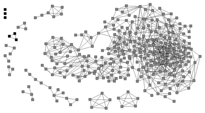
Sociometric graph of the original sample – participants not recruited into any of the 30 RDS samples are marked black.
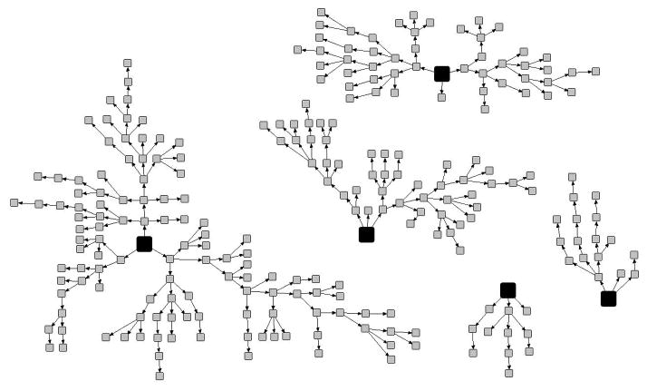
The sample sizes among the simulation samples ranged between n=246 (82.3% of participants from the original sample) and n=261 (87.3%), with the mean, median, and mode all being n=250 (83.6%). There were 11 simulation samples where the sample size was equal to or smaller than the size of the largest component of the original sample (n=249). Of these 11 simulation samples with n≤249, one sample had one seed from outside the large component and four from inside of it, while the other ten had seeds only from inside the large component and none from outside of it. In the largest simulations sample with 261 people, three seeds belonged to the large component, one seed belonged to an isolated component with 3 people, and one seed belonged to an isolated component with 12 people. Figure 2 depicts one of the simulation samples, with seeds marked as black.
Figure 2.
Recruitment chains of one of the RDS simulation samples – seeds are marked black.
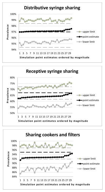
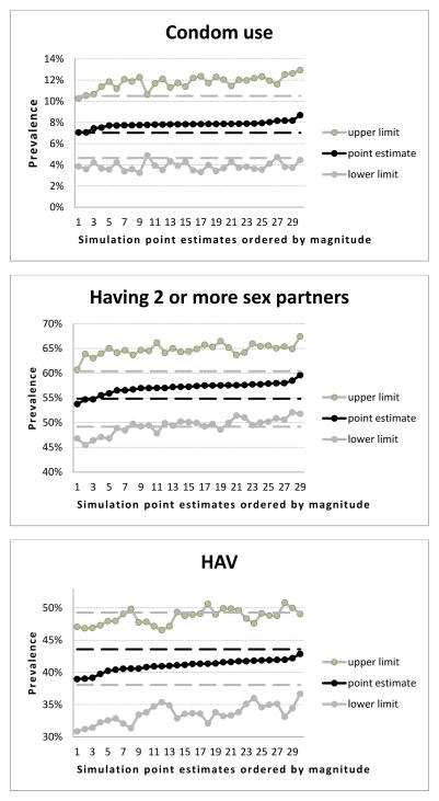
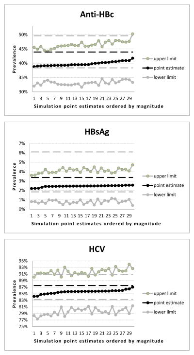
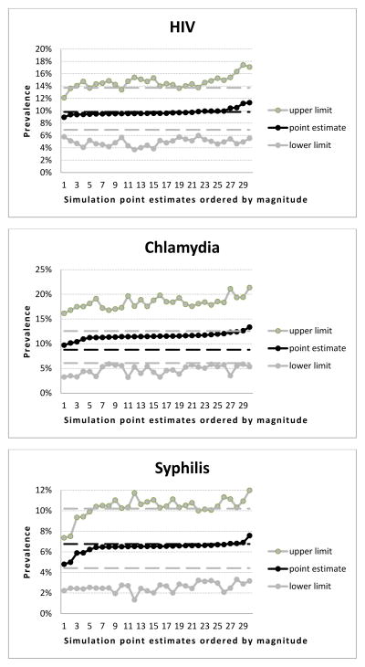
Table 1 shows the prevalence values and the 95%CI of the characteristics of interest in the original sample. Figure 3 shows the point estimates and the 95%CI of the simulation samples (chart lines with dots) and the prevalence and 95%CI in the original sample of each of the characteristics (solid vertical lines with no dots). These charts show that among the 360 simulation sample point estimates, only one was significantly smaller than the prevalence in the original sample (sharing cookers and filters), and two were significantly higher than the prevalence in the original sample (both for Chlamydia infection). Therefore, 99.2% of simulation sample point estimates were within the 95%CI of the original sample prevalence values for the variables of interest.
Table 1.
Prevalence of selected sample characteristics. People who inject drugs, Vilnius, Lithuania, March 2008–May 2009
| Characteristic | Prevalence (95% CI) |
|---|---|
| Distributive syringe sharing | 97.0% (94.4, 98.4) |
| Receptive syringe sharing | 67.2% (61.7, 72.3) |
| Sharing cookers and filters | 95.0% (91.9, 96.9) |
| Using condoms every time during sex | 7.0% (4.6, 10.5) |
| Having two or more sex partners | 54.8% (49.2, 60.4) |
| Prevalence of HAV | 43.6% (38.1, 49.3) |
| Prevalence of Hbs | 43.9% (38.4, 49.6) |
| Prevalence of HbsAg | 3.4% (1.8, 6.1) |
| Prevalence of HCV | 87.5% (83.2, 90.8) |
| Prevalence of HIV | 9.8% (6.9, 13.7) |
| Prevalence of Chlamydia | 8.8% (6.1, 12.6) |
| Prevalence of syphilis | 6.8% (4.4, 10.2) |
Figure 3.
Point estimates and 95% confidence intervals of the RDS simulations samples for selected infections and risk behaviours (past 30 days)
3a: Distributive syringe sharing
3b: Receptive syringe sharing
3c: Sharing cookers and filters
3d: Using condoms every time during sex
3e: Having two or more sex partners
3f: Prevalence of HAV
3g: Prevalence of anti-HBc
3h: Prevalence of HBsAg
3i: Prevalence of HCV
3j: Prevalence of HIV
3k: Prevalence of Chlamydia
3l: Prevalence of syphilis
- For better visualization and interpretation, point estimates of the simulation samples were ordered by magnitude (the X axis of each chart represents the rank order of the simulation sample point estimates), and only the related confidence interval ranges are depicted (therefore the Y axis ranges are different for each chart both in terms of minimum and maximum values and in terms of units within the ranges between minimum and maximum).
- Prevalence and, respectively, 95% confidence intervals for each characteristic in the original sample are represented as black and, respectively, gray vertical lines within each chart to provide a visual reference for the point estimates of the simulation samples.
- Statistically significant difference is when a point estimate of the simulation sample lies either under the lower confidence interval or above the upper confidence interval of the prevalence within the original sample for the relevant characteristic.
4. DISCUSSION
In this analysis, we simulated RDS based on an ISS of PWID in Lithuania. To our knowledge, this is the first simulation that models RDS on an actual sample of PWID. Based on the results, our two hypotheses were not confirmed. First, the majority (four in five) of the participants in the original sample was recruited into the simulation samples; and second, there was no statistically significant difference between the prevalence of selected characteristics in the original sample and the point estimates of all but three point estimates of the simulation samples.
There are several potential reasons why we were unable to confirm our hypotheses. The failure to confirm the first hypothesis is probably due to the sociometric network structure of the original sample: 83% of people in the original sample belonged to a large component, and – generally – as long as all the seeds were recruited from the large component of the original sample, the simulation samples simply recreated this large component. The failure to confirm the second hypothesis lies in the combination of two factors. First, there were no statistically significant differences between the large component and the entire original sample regarding the characteristics of interest. Therefore, since the simulation samples were dominated by the large network component of the original sample, the simulation samples were not statistically different from the original samples.
Within 30 simulation iterations, only six individuals – three isolated persons and a component with three individuals – were not recruited into any of the simulation samples. RDS has been criticized for underperforming in recruiting small networks (Paquette et al., 2012), and our findings also points to this aspect of RDS. In our simulation exercise, the exclusion of these small network components affected only 2% of the sample and without creating a statistically significant difference between the original sample and the simulated samples. However, in real-world settings in populations with lower densities or more fragmented networks, or where small networks constitute a larger proportion of the population than in this simulation study, this exclusion of small network components may lead to a statistically significant distortion of the RDS estimates compared to true population prevalences. Missing isolated network components in sampling may not bias sampling as long as the characteristics of the small networks are similar to the characteristics of the large networks, or if small networks constitute only a small proportion of the population – like in the original sample of this simulation study.
Another important finding was that only three out of the 360 simulation estimates were statistically different from their respective sample prevalence values: a 0.8% divergence, which is low enough to be due to statistical error. In that case, the difference between the simulated RDS samples and the original sample is that in the simulation samples the network ties are untangled (laid out flat into two-dimensional recruiting chains), while in the original sample they are entangled (intertwined into a three-dimensional sociometric net – see Figure 1 vs. Figure 2). This reminded us of the making of a strudel. A strudel is a filo pastry originated in Hungary: after the filling is dispersed on the thinly stretched out filo dough, the dough with the filling is rolled up carefully and baked in the oven (Wikipedia, 2013). Our figure depicting the two-dimensional RDS simulation sample recruiting waves resembles the stretched out filo dough lying flat on a table with the filling dispersed on it, while the figure depicting the three-dimensional sociometric network resembles the whirlpool-look of a rolled up strudel with the filling (the nodes of the sociometric network) interspersed among the layers of the dough (the sociometric links). What this “strudel effect” may mean in reality is that given certain social network characteristics (such as density, fragmentation, and centrality measures), RDS may produce samples with prevalence estimates that are not statistically significantly different from prevalence estimates that would be obtained by ISS.
One limitation of this simulation study is that the original sample is not the entire PWID population either in Vilnius or in Lithuania, nor may it be a representative sample of the population. Therefore, this RDS simulation exercise may simply have recreated the original research sample, most likely made up of people using the NEP. As a matter of fact, one of our findings was that (with the exception of one simulation sample) as long as all the seeds were selected from the large component of the original sample, the simulation samples simply recreated the large component. Getting stuck in a clique of strong network ties is a potential problem in RDS which may be overcome by having diversely selected seeds (i.e., those not associated with the NEP). Although if the factors associated with smaller components are not known, then RDS recruitment may unknowingly miss certain components. However, one assumption of most RDS estimators is that the sample will eventually reach equilibrium which is an indication that the sample is no longer biased by the non-randomly selected seeds (even if all of them are associated with the NEP) (Heckathorn, 1997, 2002). In our simulation samples, we had recruitment chains up to 11 waves (see Figure 2), considered as more than sufficient for RDS surveys. However, recreating (the majority of) the original sample was key in rejecting our first research hypotheses: if the original sample could be more or less recreated by simulating RDS, then RDS would probably have resulted in a similar sample had it been used to obtain the original sample. The second limitation is that this simulation study was performed based on a set of assumptions, and these assumptions may not have been met in actual sampling. For example, in this simulation participants were randomly recruiting their network members, whereas in real life there is evidence of preferential recruitment (Heckathorn 2002; Liu et al. 2012; Wang et al. 2005). For instance, PWID have been known to sell, barter, or control recruitment during surveys resulting in violations of participants having reciprocal relationships and random sampling in the network (Scott, 2008). The original sample was obtained by participants actually recruiting their actual network members. Therefore, some preferential recruitment may already have taken place in the original sample, and been reflected in the composition of the recorded sociocentric network links. Moreover, the original sample captured certain network links, and these links may have been different at the time of recruitment had the original sample been recruited using RDS. Another limitation is that the naming stimuli that were used to delineate the social network may not be sufficiently specific (e.g. people may go to different people depending on the nature of advice or favor they need: financial, professional, emotional) and missed key network members. Lastly, this simulation study could not assess overall performance of RDS vs. ISS, because the population was not enumerated. These findings do, however, point to the important role of social network structural components, which warrants further investigation.
This simulation study showed that because there were no significant differences between the large component and the entire original sample regarding the characteristics of interest, the simulation samples were not statistically significantly different from the original sample. As such, in populations where population characteristics are reflected in large network components that dominate the population, RDS and ISS may produce samples that have statistically non-different prevalence values, even though some isolated network components may be under-sampled and/or statistically significantly different from the main groups. Therefore, the goal of future (simulation) studies may be to examine the sociocentric network conditions and the threshold levels of population characteristics where sampling processes would have diverging prevalence estimates.
Footnotes
Publisher's Disclaimer: This is a PDF file of an unedited manuscript that has been accepted for publication. As a service to our customers we are providing this early version of the manuscript. The manuscript will undergo copyediting, typesetting, and review of the resulting proof before it is published in its final citable form. Please note that during the production process errors may be discovered which could affect the content, and all legal disclaimers that apply to the journal pertain.
References
- Borgatti SP, Everett MG, Freeman LC. Ucinet for Windows: Software for Social Network Analysis. Analytic Technologies; Harvard, MA: 2002. [Google Scholar]
- Des Jarlais DC, Arasteh K, Semaan S, Wood E. HIV among injecting drug users: current epidemiology, biologic markers, respondent-driven sampling, and supervised-injection facilities. Curr Opin HIV AIDS. 2009;4:308–313. doi: 10.1097/COH.0b013e32832bbc6f. [DOI] [PMC free article] [PubMed] [Google Scholar]
- Friedman SR, Curtis R, Neaigus A, Jose B, Des Jarlais DC. Social Networks, Drug Injectors’ Lives, and HIV. Plenum; New York: 1999. [Google Scholar]
- Friedman SR, Neaigus A, Jose B, Curtis R, Goldstein MF, Ildefonso G, Rothenberg RB, Des Jarlais DC. Sociometric risk networks and risk for HIV infection. Am J Public Health. 1997;87:1289–1296. doi: 10.2105/ajph.87.8.1289. [DOI] [PMC free article] [PubMed] [Google Scholar]
- Gile KJ, Handcock MS. Respondent driven sampling: an assessment of current methodology. Sociol Methodol. 2010;40:285–327. doi: 10.1111/j.1467-9531.2010.01223.x. [DOI] [PMC free article] [PubMed] [Google Scholar]
- Goel S, Salganik MJ. Assessing Respondent-Driven Sampling. Proceedings of the National Academy of Sciences. 2010;107:6743–6747. doi: 10.1073/pnas.1000261107. [DOI] [PMC free article] [PubMed] [Google Scholar]
- Gyarmathy VA, Neaigus A. The effect of personal network exposure on injecting equipment sharing among Hungarian IDUs. Connections. 2006;15:29–42. [PMC free article] [PubMed] [Google Scholar]
- Gyarmathy VA, Neaigus A, Li N, Ujhelyi E, Caplinskiene I, Caplinskas S, Latkin CA. Infection disclosure in the injecting dyads of Hungarian and Lithuanian injecting drug users who self-reported being infected with hepatitis C virus or human immunodeficiency virus. Scand J Infect Dis. 2010a;43:32–42. doi: 10.3109/00365548.2010.513064. [DOI] [PMC free article] [PubMed] [Google Scholar]
- Gyarmathy VA, Neaigus A, Li N, Ujhelyi E, Caplinskiene I, Caplinskas S, Latkin CA. Liquid drugs and high dead space syringes may keep HIV and HCV prevalence high - a comparison of Hungary and Lithuania. Eur Addict Res. 2010b;16:220–228. doi: 10.1159/000320287. [DOI] [PMC free article] [PubMed] [Google Scholar]
- Gyarmathy VA, Neaigus A, Ujhelyi E. Vulnerability to drug-related infections and co-infections among injecting drug users in Budapest, Hungary. Eur J Public Health. 2009;19:260–265. doi: 10.1093/eurpub/ckp009. [DOI] [PMC free article] [PubMed] [Google Scholar]
- Hard-to-Reach Population Methods Research Group. RDS Analyst. 2013;1.0 www.hpmrg.org. [Google Scholar]
- Heckathorn DD. Respondent-driven sampling: a new approach to the study of hidden populations. Soc Probl. 1997;44:174–199. [Google Scholar]
- Heckathorn DD. Respondent-driven sampling II: deriving valid population estimates from chain-referral samples of hidden populations. Soc Probl. 2002;49:11–34. [Google Scholar]
- Horyniak D, Higgs P, Jenkinson R, Degenhardt L, Stoove M, Kerr T, Hickman M, Aitken C, Dietze P. Establishing the Melbourne Injecting Drug User Cohort Study (MIX): rationale, methods, and baseline and twelve-month follow-up results. Harm Reduct J. 2013;10:11. doi: 10.1186/1477-7517-10-11. [DOI] [PMC free article] [PubMed] [Google Scholar]
- Kral AH, Malekinejad M, Vaudrey J, Martinez AN, Lorvick J, McFarland W, Raymond HF. Comparing respondent-driven sampling and targeted sampling methods of recruiting injection drug users in San Francisco. J Urban Health. 2010;87:839–850. doi: 10.1007/s11524-010-9486-9. [DOI] [PMC free article] [PubMed] [Google Scholar]
- Liu H, Li J, Ha T, Li J. Assessment of random recruitment assumption in respondent-driven sampling in egocentric network data. Soc Netw. 2012;1:13–21. doi: 10.4236/sn.2012.12002. [DOI] [PMC free article] [PubMed] [Google Scholar]
- Malekinejad M, Johnston LG, Kendall C, Kerr LR, Rifkin MR, Rutherford GW. Using respondent-driven sampling methodology for HIV biological and behavioral surveillance in international settings: a systematic review. AIDS Behav. 2008;12:105–130. doi: 10.1007/s10461-008-9421-1. [DOI] [PubMed] [Google Scholar]
- Montealegre JR, Johnston LG, Murrill C, Monterroso E. Respondent driven sampling for HIV biological and behavioral surveillance in Latin America and the Caribbean. AIDS Behav. 2013;17:1–28. doi: 10.1007/s10461-013-0466-4. [DOI] [PubMed] [Google Scholar]
- Paquette D, Bryant J, De Wit J. Respondent-driven sampling and the recruitment of people with small injecting networks. AIDS Behav. 2012;16:890–899. doi: 10.1007/s10461-011-0032-x. [DOI] [PubMed] [Google Scholar]
- Platt L, Wall M, Rhodes T, Judd A, Hickman M, Johnston LG, Renton A, Bobrova N, Sarang A. Methods to recruit hard-to-reach groups: comparing two chain referral sampling methods of recruiting injecting drug users across nine studies in Russia and Estonia. J Urban Health. 2006;83:39–53. doi: 10.1007/s11524-006-9101-2. [DOI] [PMC free article] [PubMed] [Google Scholar]
- Scott G. They got their program, and I got mine”: a cautionary tale concerning the ethical implications of using respondent-driven sampling to study injection drug users. Intl J Drug Policy. 2008;19:42–51. doi: 10.1016/j.drugpo.2007.11.014. [DOI] [PubMed] [Google Scholar]
- Sifaneck S, Neaigus A. The ethnographic accessing, sampling and screening of hidden populations: heroin sniffers in New York City. Addict Res Theor. 2001;9:519–543. [Google Scholar]
- Wang J, Carlson RG, Falck RS, Siegal HA, Rahman A, Li L. Respondent-driven sampling to recruit MDMA users: a methodological assessment. Drug Alcohol Depend. 2005;78:147–157. doi: 10.1016/j.drugalcdep.2004.10.011. [DOI] [PubMed] [Google Scholar]
- Wikipedia. [Accessed: October 29, 2013];Strudel. 2013 http://en.wikipedia.org/wiki/Strudel.
- Wilson EB. Probable inference, the law of succession, and statistical inference. J Am Stat Assoc. 1927;22:209–212. [Google Scholar]
- Wylie JL, Jolly AM. Understanding recruitment: outcomes associated with alternate methods for seed selection in respondent driven sampling. BMC Med Res Methodol. 2013;13:93. doi: 10.1186/1471-2288-13-93. [DOI] [PMC free article] [PubMed] [Google Scholar]
- Young AM, Jonas AB, Mullins UL, Halgin DS, Havens JR. Network structure and the risk for HIV transmission among rural drug users. AIDS Behav. 2012;17:2341–2351. doi: 10.1007/s10461-012-0371-2. [DOI] [PMC free article] [PubMed] [Google Scholar]


