

Abstract
Static whole body PET/CT, employing the standardized uptake value (SUV), is considered the standard clinical approach to diagnosis and treatment response monitoring for a wide range of oncologic malignancies. Alternative PET protocols involving dynamic acquisition of temporal images have been implemented in the research setting, allowing quantification of tracer dynamics, an important capability for tumor characterization and treatment response monitoring. Nonetheless, dynamic protocols have been confined to single bed-coverage limiting the axial field-of-view to ~15–20 cm, and have not been translated to the routine clinical context of whole-body PET imaging for the inspection of disseminated disease. Here, we pursue a transition to dynamic whole body PET parametric imaging, by presenting, within a unified framework, clinically feasible multi-bed dynamic PET acquisition protocols and parametric imaging methods. We investigate solutions to address the challenges of: (i) long acquisitions, (ii) small number of dynamic frames per bed, and (iii) non-invasive quantification of kinetics in the plasma. In the present study, a novel dynamic (4D) whole body PET acquisition protocol of ~45min total length is presented, composed of (i) an initial 6-min dynamic PET scan (24 frames) over the heart, followed by (ii) a sequence of multi-pass multi-bed PET scans (6 passes x 7 bed positions, each scanned for 45sec). Standard Patlak linear graphical analysis modeling was employed, coupled with image-derived plasma input function measurements. Ordinary least squares (OLS) Patlak estimation was used as the baseline regression method to quantify the physiological parameters of tracer uptake rate Ki and total blood distribution volume V on an individual voxel basis. Extensive Monte Carlo simulation studies, using a wide set of published kinetic FDG parameters and GATE and XCAT platforms, were conducted to optimize the acquisition protocol from a range of 10 different clinically acceptable sampling schedules examined. The framework was also applied to six FDG PET patient studies, demonstrating clinical feasibility. Both simulated and clinical results indicated enhanced contrast-to-noise ratios (CNRs) for Ki images in tumor regions with notable background FDG concentration, such as the liver, where SUV performed relatively poorly. Overall, the proposed framework enables enhanced quantification of physiological parameters across the whole-body. In addition, the total acquisition length can be reduced from 45min to ~35min and still achieve improved or equivalent CNR compared to SUV, provided the true Ki contrast is sufficiently high. In the follow-up companion paper, a set of advanced linear regression schemes is presented to particularly address the presence of noise, and attempt to achieve a better trade-off between the mean-squared error (MSE) and the CNR metrics, resulting in enhanced task-based imaging.
1. Introduction
Clinical diagnosis and treatment response monitoring of localized and metastatic cancer malignancies have remarkably benefited from the advent of whole-body positron emission tomography, integrated with computed tomography (PET/CT) imaging (Wahl and Buchanan 2002). The standardized uptake value (SUV) is currently widely employed in the clinic, as a surrogate of metabolic activity, across multiple bed positions, enabling whole-body imaging (Facey et al 2007, Castell and Cook 2008). The PET acquisition associated with the SUV metric is static, i.e. every bed position is scanned once, typically around and/or after one hour post-injection (Dahlbom et al 1992, Kubota et al 2001, Hustinx et al 2002, Townsend 2008). Meanwhile, increasing efforts are devoted towards transition of qualitative reads towards quantitative SUV assessment, especially for treatment response assessment (e.g. extensive review by Wahl et al 2009).
At the same time, the quantitative accuracy of SUV estimates relies primarily on two conditions: (i) in the voxel or region of interest (ROI), contribution of non-metabolized tracer is negligible relative to the metabolized tracer, and (ii) time integral of plasma tracer concentration is proportional to the injected amount of tracer normalized by the body weight (or lean body mass or body surface area) (Zasadny and Wahl 1993, Kim et al 1994, Kim and Gupta 1996, Sadato et al 1998). In clinical PET, these assumptions can fail, resulting in non-negligible errors in tracer uptake rate estimation (Leskinen-Kallio et al 1992, Hamberg et al 1994, Keyes 1995, Weber et al 1999, Huang 2000, Adams et al 2010). Overall, PET tracer distribution is a dynamic process altered by a number of factors that may be uniquely specific to each organ and region of interest (e.g. tumors), patient and time of scan, and static SUV imaging cannot always accurately account for these effects. Specifically, dynamic imaging methods have the potential to reduce the notable time-dependence observed in SUV quantification of normal tissue and tumor uptakes values, and thus may allow greater flexibility and reliability in clinical practice.
In the research setting, single bed dynamic PET imaging has been applied to capture the tracer kinetics, by scanning at a particular bed position over a sequence of time frames. For this purpose, two types of activity concentrations need to be measured across all dynamic time frames: (i) the blood plasma activity concentration, i.e. the input function, and (ii) the activity concentration of each ROI, or each voxel, i.e. the time activity curve (TAC). Subsequent analysis using an appropriate kinetic model can result in more quantitative parameter estimates, compared to SUV imaging (Wong and Hicks 1994, Sadato et al 1998, Dimitrakopoulou-Strauss et al 2001). Nonetheless, dynamic PET protocols have been confined to single bed-coverage limiting the axial field-of-view of the parametric images to ~15–20 cm, and have not yet been translated to the routine clinical context of multi-bed PET imaging for the inspection of disseminated disease, which is a significant component of PET imaging nowadays.
In the current work, we pursue a transition from static to dynamic whole-body PET imaging, in clinically feasible total scan times, and focus on parametric imaging at the individual voxel level. The proposed approach, aside from covering a large axial field of view, enables truly quantitative dynamic imaging which can be crucial in both diagnosis and treatment response monitoring (Castell and Cook 2008). For instance, detection and quantification of small lesions imaged using FDG PET (e.g. lesions following therapy) in the liver and mediastinum can be challenged due to considerable background uptake. Dynamic imaging can remove this background uptake as there is a time dependent signature difference between normal tissue and tumor, and between blood pool and tumor, and subsequently it can allow for small and less FDG avid tumors to be more easily identified in contrast to the challenges faced in the “sea of background” situation seen in standard SUV PET imaging.
To achieve 4D whole body PET acquisition, the following three challenges need to be addressed: (i) long acquisitions, (ii) few number of dynamic frames at each bed, and (iii) non-invasive quantification of rapid early kinetics in the plasma. A particular study by Ho-Shon et al (1996) was notable as it proposed a method to optimize multi-bed dynamic PET acquisitions, based on a statistical Bayesian regression method. This approach, however, was focused towards ROI-based parametric analysis and included demonstration of 2-bed acquisition examples with uneven bed frames and bi-directional scanning. Kaneta et al (2007) also conducted multi-bed dynamic acquisition of human subjects (0–90min post-injection) in the context of imaging hypoxia using 18F-FRP170, involving sequential whole-body acquisitions, each lasting for 12min (6 beds x 2min/bed). However, only dynamic images were presented, and tracer kinetic modeling or scanning protocol optimization was not performed.
In the current study, a novel 4D whole body PET acquisition protocol is proposed (Sec. 2.2) enabling input function estimation as well as generation of dynamic whole-body datasets. An extensive set of Monte Carlo simulation studies was conducted, incorporating realistic kinetics obtained from an extensive literature review, to optimize this 4D acquisition protocol, based on quantitative analysis. Later, the optimized protocol was applied to six FDG PET patient studies, demonstrating clinical feasibility (Karakatsanis et al 2011). Standard Patlak linear graphical analysis modeling was employed at the voxel level, coupled with plasma input function estimation from the images, to estimate the tracer uptake rate Ki (slope) and the total blood distribution volume V (intercept) (Patlak et al 1983, Patlak and Blasberg 1985, Zhou et al 2010). Patlak modeling can be a powerful tool in the present context of dynamic whole-body imaging, as it only requires the measurement of the later part of each voxel time activity curve, thus alleviating the need for early dynamic scanning of all beds, which is very challenging in dynamic whole-body PET.
2. Dynamic whole-body PET acquisition
2.1. SUV (static) vs. Patlak (dynamic) PET imaging
The SUV metric is defined as:
| (1) |
where, C(t) is the tracer concentration, decay corrected with respect to the tracer injection time, Dose is the amount of injected activity and LBM is the lean body mass. Due to its simplicity, SUV is widely used in conventional static whole body clinical FDG studies. However, in reality SUV: (i) cannot differentiate between non-metabolized and metabolized tracer concentrations, and (ii) does not take into account the plasma dynamics (Sadato et al 1998, Zasadny and Wahl 1993, Kim and Gupta 1996, Kim et al 1994).
As a result, the SUV can be considered a semi-quantitative surrogate of the metabolic rate in certain cases in clinical FDG PET imaging (Hamberg et al 1994, Keyes 1994, Huang 2000). For instance, if a patient is undergoing chemo- or hormone-therapy, and has impaired renal function, the clearance of plasma FDG could be significantly reduced and, therefore, the total amount of FDG in blood plasma available for absorption could be larger than what would be predicted from the injected dose and lean body mass alone (eq.1). In such a case, SUV will overestimate the metabolic rate of glucose in tumor (Leskinen-Kallio et al 1992, Weber et al 1999, Huang 2000, Adams et al 2010). Thus, the therapy response may not be accurately reflected by SUV.
On the contrary, quantitative parametric imaging dynamically acquires a time series of PET measurements (4D acquisition) and, subsequently, utilizes kinetic modeling techniques, to estimate, at the voxel level, physiological parameters of interest. The standard 2-tissue-compartment kinetic model with irreversible tracer metabolism (k4 ≃ 0) has been employed (figure 1) to describe the FDG kinetics.
Figure 1.
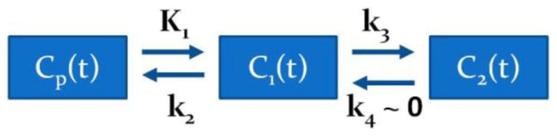
A graph for the compartment model of 18F-FDG tracer uptake. Cp(t), C1(t) and C2(t) are the tracer concentration in plasma, free (reversible) and metabolized (irreversible, k4 ~ 0) compartments respectively.
The tracer activity concentration in both the blood plasma, Cp(t), and the tissue, C(t), are measured over time. Then, the tracer metabolic rate is estimated by applying linear regression methods to the Patlak equation for t ≥ t* (t* is the time after which relative equilibrium is attained between the vascular space and reversible tissue compartment) (Patlak et al 1983, Patlak and Blasberg 1985):
| (2) |
The parameters Ki and V are the slope and intercept of linear regression respectively. In the case of FDG tracer, Ki represents the tracer influx or uptake rate constant in the tissue, while V is the total blood plasma distribution volume, i.e. the sum of the distribution volume of the reversible compartment and the fractional blood plasma volume present in the tissue. The standard Patlak model (Patlak et al 1983) assumes the 2-compartment kinetic model with irreversible uptake (figure 1) for the underlying tracer kinetics, i.e. k4=0, a reasonable approximation for FDG tracer kinetics for most regions and tumors.
Patlak standard model is a fast linear graphical analysis method, hence, appropriate for estimation at the voxel level of the Ki and V parameters and for production of quantitative parametric images of glucose uptake rates across all bed positions. By comparing (1) and (2), it is evident that, unlike SUV, Ki parametric imaging takes into account the plasma FDG dynamics.
Furthermore, Patlak graphical analysis is powerful in the present context of dynamic whole-body PET imaging, as it only requires the measurement of each voxel time activity curve after kinetic equilibrium is attained, thus alleviating the need for dynamic scanning of all beds within the first few minutes post injection, which is not feasible for dynamic multi-bed acquisitions. In addition, the process of non-linear estimation of the kinetic micro-parameters K1, k2 and k3 reduces to linear regression, requiring fewer temporal samples, to determine the macro-parameters Ki and V.
2.2. Dynamic (4D) whole-body PET acquisition
2.2.1. Design of the acquisition protocol
The transition from single- to multi-bed PET parametric imaging poses significant challenges for the data acquisition including the long scan duration and the small number of frames per bed position. A preliminary feasibility study conducted by our group (Zhou et al 2010) had demonstrated that whole-body Patlak Ki images produced with a 10–60min 2-bed dynamic protocol were comparable to the images estimated from a continuous single-bed dynamic study of the same length. In this study, we are investigating a set of novel 4D whole-body acquisition schemes designed to efficiently address the existing challenges, while targeting clinical feasibility and adoption. For this purpose, we are examining different number of dynamic frames per bed position and various total study durations, while ensuring compliance to clinical requirements.
The GE Discovery RX LYSO PET/CT scanner, located at Johns Hopkins PET center, was used for this study. The total acquisition time for the 4D whole-body PET acquisition is ~48min and is implemented in two subsequent time phases (Karakatsanis et al 2011, 2012a):
An initial 6-min single-bed dynamic scan over the cardiac region comprised of 24 frames with the following time sequence: (12 frames) x (10sec) + (12 frames) x (20sec), in order to later extract, the early tracer dynamics in the blood plasma, followed by
A sequence of 6 whole-body scans (passes), each lasting approximately 6min and comprised of seven beds, each scanned for 45sec, to capture the late dynamics of the tracer in both the blood plasma and the tissues.
All dynamic frames of the second phase are equal. Moreover, all whole body passes are performed uni-directionally (cranio-caudal scanning) as bi-directional scanning was found (Zhou et al 2010) to result in inconsistent regression statistics across the beds (due to a resulting non-uniform temporal sampling across the beds). As a result, each bed position is scanned for same number of times, non-continuously and with equal sampling frequency. An acquisition time gap of 80sec exists between subsequent passes, which corresponds to the time required for the scanner to (i) return to the initial bed position after the completion of each whole-body pass and (ii) to revert back to the 3D mode (as the septa come out at the end of each pass for this particular scanner; an issue that can be addressed with appropriate system upgrade and avoided in septa-less PET scanners). The acquisition time sequence for the second phase is illustrated in figure 2.
Figure 2.

Illustration of the acquisition time sequence for the later 6 whole-body passes (second phase of the protocol). Each row describes the acquisition of a particular whole-body pass over time (only 3 of the 6 passes are shown). The time is running row-wise. Note that every pass consists of 7 bed positions. Each column corresponds to one bed position. The earlier dynamic scan is performed on bed 3, for the first 6min after injection, and is not shown here.
The initial dynamic scan (the first acquisition phase) tracks the rapid kinetics of the input function during the first 6min after injection, while the subsequent, smoother portion of the input function is determined from the dynamic images corresponding to the cardiac bed in the second acquisition phase (figure 2, bed 3). ROIs are drawn over the left ventricle (LV) in all dynamic cardiac frames of the two acquisition phases to extract the input function measurements. The input function for the first acquisition phase is approximated by applying linear interpolation on the first 24 extracted LV ROI mean values. Similarly, for the second phase, linear interpolation is applied on the last 6 LV ROI mean values to approximate the input function value at each dynamic frame of the rest of the beds. We selected the LV region, allowing us to draw relatively large cubic ROIs (4x4x4 voxels; ~2.5cm3), while maintaining an adequate distance between the ROI edges and the myocardium. The large size and the distance from the myocardium ensure minimal bias due to spill-in of myocardial activity while reducing noise in the mean estimates, as indicated by an example of a patient input function plot presented in figure 3(a). It should be noted that the FDG tracer input function is not varying considerably during the second phase of acquisition (10–45min) and therefore 6 measurements are sufficient for the interpolation process. Also linear interpolation produced same performance with cubic spline interpolation. The very initial inclination of the input function curve is not observed in the plot as the acquisition of the first dynamic frame started ~20sec after injection. This delay was necessary due to the fact that the patients were scanned with arms down for their convenience given the relatively long acquisition. Consequently, they had to be repositioned right after injection to conduct the dynamic cardiac scan, as the site of injection was not accessible with the arms down, if the cardiac region was to be within the FOV. However the area under curve for the first 20sec is very small compared to the total integral of the input function at later time points and, thus, the resulting error in integration and in parameter estimation may be negligible.
Figure 3.
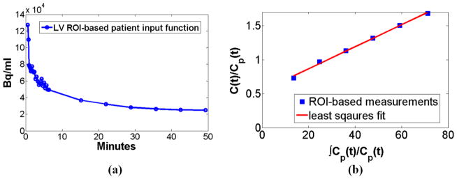
(a) A patient input function as extracted from LV ROIs drawn on the 30 dynamic cardiac frames of our proposed optimized whole-body acquisition protocol. (b) Patlak plot obtained from the previous input functions measurements and a patient tumor ROI drawn on the last 6 frames of a bed.
Due to high activity concentration over the heart immediately after injection and relatively lower concentration in the tissues later on, the capability of the GE RX scanner to retract its septa and, therefore, support both 2D and 3D acquisition mode was utilized, to maintain a relative high detection efficiency throughout the acquisition time. In particular, the dynamic scan over the heart is performed in 2D acquisition mode to reduce dead time effects and large number of randoms (improve NEC performance), while the subsequent whole-body data are acquired in 3D mode. As we later discuss in section 6.1.3 and also observe from an example of a patient input function in figure 3a, the input function measurements acquired for the two phases are expected to be quantitatively comparable. However, as the PET scanner has to switch from 2D to 3D acquisition mode during each study, a time span of 100sec is required to retract the detector septa, during which no acquisition takes place. In the case of simulation studies, the data of the first and second phase were also acquired in 2D and 3D modes respectively. The details of our simulation studies set-up are described in section 4.1.
2.2.2. Time assignment for slices in the overlap space between adjacent beds
In the case of single-bed dynamic acquisition, the counts of all slices of a bed at each time frame i are assigned the same time point , which is the average of the start time and end time of the particular frame. However, in multi-bed PET scanning, the acquisition system imposes overlaps between adjacent bed positions, i.e. certain number of edge slices belong to two adjacent bed positions, and therefore, will be scanned twice over time to enhance the lower sensitivity associated with the edge slices especially in 3D-mode bed acquisitions. For these slices, a portion of the counts are acquired at a current time frame i, while the remaining are acquired at time frame i+1. We assigned an intermediate time point to these slices:
| (3) |
where and are the middle time points of frames i and i+1. The separate time assignment for the overlapped slices effectively defines an additional intermediate bed position between each pair of adjacent original beds characterized by mid-time point . This approximation is considered satisfactory, as the FDG tracer concentration is not varying significantly between adjacent beds during the second acquisition phase.
2.2.3. Optimization of acquisition protocol (simulated study)
Currently we opt for schemes involving acquisitions starting immediately after tracer injection and not exceeding 50min, though our ultimate aim, as demonstrated in our results section 5.2, is to achieve shorter acquisition of ~30min. For comparative evaluation purposes, an SUV scan 60min post injection was also acquired. The protocol was optimized based on simulated studies elaborated in section 4. Our optimization strategy consists of two steps:
Initially, we investigate a range of number of whole-body passes from two to eight, always ensuring the total acquisition length is approximately 45min. As a result, the duration of the bed frames decreases with increasing number of passes. The scheme with the best performance is selected as optimal. Subsequently, the time frame length associated with the optimal protocol is kept constant. Then we repeat the acquisition, by omitting the last dynamic frame every time, until we have only 2 passes per bed.
The acquisition schemes selected along with the range of parameter values examined are listed in Table I. The protocols have been assigned names in the format NPx_TFy, where x and y stand for number of passes per bed, or NP, and time frame length in sec, or TF, respectively. Also the total study time TT for each protocol is presented. The left and right section of the table are associated with the first and second step of the optimization process, respectively.
Table I.
Acquisition Schemes for Dynamic Multi-Bed PET
| Protocol | NP | TF(sec) | TT(min) |
|---|---|---|---|
| NP8_TF31 | 8 | 31 | 48 |
| NP7_TF38 | 7 | 38 | 48 |
| NP6_TF45 | 6 | 45 | 48 |
| NP5_TF58 | 5 | 58 | 48 |
| NP4_TF76 | 4 | 76 | 48 |
| NP3_TF106 | 3 | 105 | 48 |
| NP2_TF165 | 2 | 165 | 48 |
| NP6_TF45 | 6 | 45 | 48 |
| NP5_TF45 | 5 | 45 | 40 |
| NP4_TF45 | 4 | 45 | 33 |
| NP3_TF45 | 3 | 45 | 26 |
| NP2_TF45 | 2 | 45 | 19 |
3. Baseline methods for whole body parametric imaging
3.1. Ordinary Least Squares regression
Let us formulate Patlak linear eq. (2) in the bi-linear form:
| (4) |
By considering eq. (2) and (4), we can arrive at the standard model for linear regression
| (5) |
| (6) |
where X is an n ×m independent variable matrix, n are the dynamic frames at times ti, i = 1,…n, at each bed position and m= 2 are the number of unknown regression parameters (Patlak slope and intercept parameters). According to the optimized protocol NP6_TF45, as presented in the results section, we consider n= 6 number of passes per bed. Furthermore, Y is a n×1 vector of known predictor variables, β is a m×1 vector of unknown regression parameters, ε is n×1 vector of experimental errors, following the normal distribution, σ2 is the error variance and In is a n ×n identity matrix.
The conventional estimator for regression parameter vector β is the ordinary least squares (OLS) estimator βOLS, given by equation (7), which minimizes the residual sum of squares RSS or ϕ:
| (7) |
| (8) |
The OLS estimator βOLS is characterized as the best linear unbiased estimator (BLUE), because its expected value is equal to the true unknown regression parameter vector β, and has the minimum variance among all linear unbiased estimators, when ε is normally distributed. However βOLS is not necessarily associated with the minimum mean squared error (MSE), a quantitative metric both accounting for bias and variance:
| (9) |
Although the associated bias in the OLS estimates is expected to be zero, the noise induced by the short bed frames, the small number of passes per bed and the voxel-wise estimation process may be large resulting in a significant increase of the MSE in the whole-body Ki images. Therefore, in the follow-up companion paper to this work (Karakatsanis et al 2013b) we focus on the development of a set of advanced linear regression methods to considerably limit the noise at the expense of a small non-zero bias in the estimates, leading to reduced MSE and improved CNR in the parameter estimates, enabling more quantitative, contrast-enhanced whole body PET parametric imaging.
3.2. Kinetic correlations based clustering
The weighted Patlak correlation coefficient (WR) of the time activity curve at each voxel is calculated in order to quantify the goodness of fit of the tracer kinetics to the Patlak model. By setting in equation (2) xi and yi, i = 1,…,n= 6 as follows:
| (10) |
the Patlak kinetics WR can be calculated at each voxel from the following equation (Zasadny and Wahl 1996) to generate a Patlak WR image:
| (11) |
where wi=(framei_duration)2/(framei_counts).
The derived WR image is utilized to group all voxels into two clusters by comparing their associated WR value with a user-defined reference correlation level. Thus, two clusters of image voxels are shaped, each characterized by a certain degree of Patlak correlation: the high (hWR) and low (lWR) kinetic correlation clusters. Voxels belonging to the hWR cluster are more likely to be associated with high uptake rate regions, such as tumors, or, overall, regions with sufficient count statistics and smooth TACs. On the contrary, the lWR cluster is expected to include voxels with insufficient Patlak correlation corresponding to noisy TACs due to low count statistics, such as tumor background regions or, overall, regions exhibiting very low uptake and, therefore, associated with relatively noisy TACs.
The performance of the WR based methods, presented in the following section as well as in the companion paper (Karakatsanis et al 2013b), rely on the selection of an “appropriate” WR reference value to best match the two clusters with the statistical quality properties assumed above. However, for different contrast regions, the “optimal” WR reference value may vary to a certain degree. Therefore, it is highly recommended that an appropriate range of reference values should be proposed to cover a reasonable set of patient tumor contrasts and, thus, ensure a reasonable agreement between the actual average statistical quality of each cluster and the expected statistical quality implied by the method.
3.3. Kinetic Correlation Driven Thresholding
Tumor or high-uptake regions with sufficient count statistics are usually associated with voxels belonging to the hWR cluster. On the contrary, background or low-uptake regions usually exhibit low Patlak kinetic correlation due to low count statistics combined with short frames and more likely belong to the lWR cluster.
By thresholding the lWR cluster voxel values to zero, the tumor contrast and detectability can potentially be enhanced, as proposed in the past for single-bed dynamic FDG PET studies (Zasadny and Wahl 1996). In this study, we extend this method to the whole-body dynamic domain and discuss a flexible strategy for task-based selection of the most appropriate WR reference value to ensure a satisfactory trade-off between contrast and quantification in the resulting thresholded whole-body parametric images. Figure 4 illustrates the flow chart of the proposed whole-body WR-based thresholding algorithm. The potential effects of WR-based thresholding and the previous strategy are discussed in the results and discussion sections.
Figure 4.

A flow chart demonstrating application of Patlak correlation-coefficient(WR)-based thresholding on the clinical whole-body parametric images. Initially the WR image is calculated and WR clustering is performed. Subsequently, WR at each voxel is compared against a user-defined threshold and, if it is higher, the original parameter value is retained in the thresholded image, otherwise the zero value is assigned to the voxel. The resulting WR-based thresholded Ki image, is compared against standard Ki image. A WR reference value (WR_threshold) of 0.85 has been used for the particular patient data.
4. Simulation Studies
4.1. Production of simulated data
We employed the Geant4 Application for Tomography Emission (GATE), a well-validated MC simulation package, to model the GE Discovery RX LYSO PET/CT scanner. GATE platform inherits the physics process models of Geant4, a generalized simulation toolkit supported by a large community of active developers, to develop simulations of nuclear medicine detector systems. Its ability to model time-dependent phenomena as well as its accurate description of all physics processes underlying emission tomography (Jan et al 2011) makes it an ideal solution for evaluation of PET/SPECT systems performance and optimization of acquisition protocols (Karakatsanis et al 2006, 2009, Sakellios et al 2006, Gonias et al 2007).
Furthermore, the realistic XCAT human torso phantom was utilized to model the attenuation as well as the time-dependent activity maps for specific tissues and tumors commonly examined in oncology whole-body PET studies (Segars et al 2010). In the current study, no cardiac or respiratory motion of the phantom has been simulated. Figure 5 shows characteristic examples of a whole-body 4D XCAT phantom. Both GATE and XCAT are state-of-the-art software platforms capable of producing, when combined with realistic sets of kinetic parameter values, realistic simulated dynamic PET multi-bed data.
Figure 5.

An example of a whole-body 4D XCAT phantom in standalone view (left and center) and visualized inside a GATE simulated gantry
For this purpose, the dynamics of the activity distribution assigned to each region of the XCAT phantom were based on actual FDG kinetic micro-parameter and effective blood plasma volume values, as reported in literature and presented in Table II (Torizuka et al 1995, Sugawara et al 1999, Dimitrakopoulou-Strauss et al 2001 and 2004 and 2006, Okazumi et al 2009, Strauss et al 2007 and 2008, Qiao et al 2007).
Table II.
FDG Kinetic Micro-Parameters
| Acquisition optimization | Parametric imaging methods | ||||||||||
|---|---|---|---|---|---|---|---|---|---|---|---|
|
| |||||||||||
| Regions | K1 | k2 | k3 | k4 | Vp | Regions | K1 | k2 | k3 | k4 | Vp |
| Normal Liver | 0.331 | 0.44 | 0.017 | 0.018 | - | Normal Liver | 0.864 | 0.981 | 0.005 | 0.016 | - |
| Liver Tumor | 0.242 | 0.388 | 0.061 | 0.022 | - | Liver Tumor | 0.243 | 0.78 | 0.1 | 0 | - |
| Normal Lung | 0.108 | 0.735 | 0.016 | 0.013 | 0.017 | Normal Lung | 0.108 | 0.735 | 0.016 | 0.013 | 0.017 |
| Lung Tumor | 0.301 | 0.864 | 0.047 | 0.001 | 0.066 | Lung Tumor | 0.044 | 0.231 | 1.149 | 0.259 | - |
| Myocardium | 0.6 | 1.2 | 0.1 | 0.001 | - | Myocardium | 0.6 | 1.2 | 0.1 | 0.001 | - |
For the acquisition optimization study (section 5.2), we have used the parameter values presented in the left column of Table II, which were obtained from an early literature search and are sufficient for the purpose of acquisition optimization. However for the evaluation of the effect of WR-based thresholding and the number of passes per bed on the Ki images (section 5.3) as well as for the companion study (Karakatsanis et al 2013b) we have utilized an updated set of kinetic parameters (right column, Table II) for the lung and liver tumor and their background regions, as selected from an extended and more up-to-date literature review. Different sets of kinetic parameters were employed for the two independent studies to demonstrate the feasibility and potential of the proposed imaging framework for a wider and more representative set of kinetic parameters. In addition, the two studies are independent from each other, and this approach ensures higher utilization of the available kinetic data available in the literature.
For the protocol optimization study, a liver and lung spherical tumor region of 10mm diameter were simulated. On the left side of the flow chart of figure 6, two sets of noise-free TAC data points are presented, as generated by the “nearly irreversible” 2-tissue compartment kinetic model (also in figure 1), using as input the kinetic parameter values of the (figure 6, upper left) the left and (figure 6, bottom left) the right column of Table II. Later, the modeled TACs were assigned accordingly to each voxel of the XCAT phantom to produce a series of activity maps later passed to the MC simulations. As a result, the total number of simulated events were determined by the noise-free TACs assigned to the XCAT phantom voxels. On the right of figure 6, an example of true activity maps from XCAT phantom is illustrated for the cardiac bed position at times corresponding to the NP6_TF45 protocol.
Figure 6.

(middle left) The 2-compartment PET tracer kinetic model and the resulting true time activity curves (TACs) for a collection of tumor and background regions for (upper left) acquisition optimization study and (bottom left) the statistical estimation study. (right) The true activity distribution for the last 6 dynamic frames of the cardiac bed position at times specific to NP6_TF45 protocol.
The simulated list-mode PET data generated by GATE were binned into 3D sinograms, according to the time frame sequence specified by each proposed acquisition scheme. Subsequently, each of the dynamic sinograms was resampled based on the bootstrap method and the noise properties of the Poisson distribution to produce multiple noise realizations (Efron and Tibshirani 1993, Haynor and Woods 1989). Then, all dynamic sinograms of all noise realizations were reconstructed using the OS-MAP-OSL algorithm implemented in STIR v2.2, an open-source software toolkit (Thielemans et al 2006), though the Bayesian beta parameter is set to 0, thus effectively rendering the OS-EM algorithm. For this simulation study and scanner a total of 21 subsets were used, as is also the case with the standard clinical data. The 315 angular bins of the GE Discovery RX scanner standard projection data format were interleaved across 21 subsets, each consisting of 15 angular bins, which were later fed to an ordered-subset (OS)-EM reconstruction algorithm to accelerate convergence of the updated image estimates. Up to 10 full iterations were performed, in order to enable generation of noise vs. bias trade-off curves. The known distributions of simulated scatter and random events were removed from prompts sinogram to determine the simulated trues sinograms. Finally, the trues sinogram data were corrected for normalization and attenuation effects by utilizing a normalization sinogram for the particular scanner and the XCAT attenuation map respectively. The resulting correction factors were incorporated into the sensitivity image of the OS-EM algorithm.
4.2. Quantitative optimization criteria
The choice of the optimal acquisition protocol was based on the quantitative criteria of the normalized bias (NBias) and the normalized standard deviation (NSD), which were utilized to quantify the bias and the noise in particular ROIs of the derived parametric Ki image from each protocol. For the simulated data, where the true Ki is known, the normalized bias (NBias) of each region can be determined by first calculating NBiasi for the ith voxel of an ROI over all R noise realizations and, subsequently, averaging over all voxels of that ROI:
| (12) |
where denotes the ith voxel value from rth noise realization, μi denotes the reference true ith voxel, n is the number of voxels in the ROI and R is the number of noise realizations. Furthermore, for the calculation of the normalized standard deviation NSD of simulated ROIs, first the NSDi of the ith voxel was calculated over all R realizations, followed by an averaging over all n voxels of the ROI:
| (13) |
Similarly, the normalized MSEi (NMSEi) was first calculated for each ith voxel over all realizations, followed by spatial averaging over all voxels of the ROI to yield the NMSE for that ROI (equation 14).
| (14) |
For the clinical data, where only a single realization (R=1) was available, a spatial NSD of an ROI is calculated from the following equation, where and fi denotes the ith voxel intensity:
| (15) |
By comparing equations 13 and 15, it should be pointed out that NSD quantifies noise across multiple realizations of an ROI for each voxel, while NSDspatial, also known as ROI roughness, measures the noise across all voxels of a single realization of an ROI. Subsequently NSD and NSDspatial can be averaged over all voxels of the ROI and over all noise realizations of that ROI, respectively. The overall NBias, NSD and NMSE metrics for each image are defined as the weighted average of individual ROIs metrics. The sizes of the ROIs are employed as weights.
These quantitative calculations were repeated for parametric images derived from all examined protocols and from a range of OSEM iterations of the original dynamic PET images. Then, NSD was plotted against NMSE for a set of parametric images corresponding to the same protocol but to different number of OSEM iterations in order to produce each noise vs. bias curve. The protocol associated with the curve closer to the origin of the axes was considered the optimal.
Finally, the metric of contrast to noise ratio CNR has been applied to evaluate the tumor detectability in both simulated and clinical parametric images from extracted ROIs in tumor and background regions:
| (16) |
5. Results
5.1 Clinical Demonstration of SUV against Patlak Ki PET imaging
In the current section we present results from clinical dynamic whole-body FDG PET/CT scans performed in our PET center to demonstrate the clinical feasibility of the proposed acquisition schemes as well as to validate the optimized protocol. Figure 7 summarizes results from a patient characterized by a high uptake lung tumor with low background. The SUV image is compared against two whole body Ki images obtained from six and four dynamic frames per bed respectively. From qualitative inspection of the clinical images, it is evident in all clinical cases that counts in large regions (e.g. liver) originally exhibiting high non-malignant uptake in SUV images, are substantially suppressed in Ki images, demonstrating the potential of the proposed imaging framework in diagnosing tumors in those regions.
Figure 7.
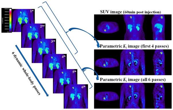
(left) the last 6 whole body dynamic frames as acquired with NP6_TF45 protocol, (right): The SUV image, the Ki parametric image derived from all 6 last frames and the Ki image after omitting the last 2 frames. Note that the patient tumor region here (lung tumor) corresponds to the third class of contrast environments, as discussed in section 6.2, and is expected to exhibit similar CNR levels both in SUV and Ki imaging.
In order to quantitatively assess contrast enhancement in the parametric Ki images vs. SUV, three suspected tumor regions were identified from a subset of clinical FDG studies and the corresponding ROI-based tumor-to-background contrast and CNR measurements were extracted (figure 8). The results suggest enhanced CNR for the Ki images for two of the examined tumor regions, characterized by high-uptake foci and low background activity (figure 8, ROI 2 and 3). However, for one of the ROIs which is located at the bowel (figure 8, ROI 1), SUV images exhibited higher CNR, possibly due to the effect of continuous and irregular bowel motion often observed in certain patients (Nakamoto et al 2004), which can be more drastic for long acquisitions, as is the case with dynamic multi-bed PET/CT protocols.
Figure 8.
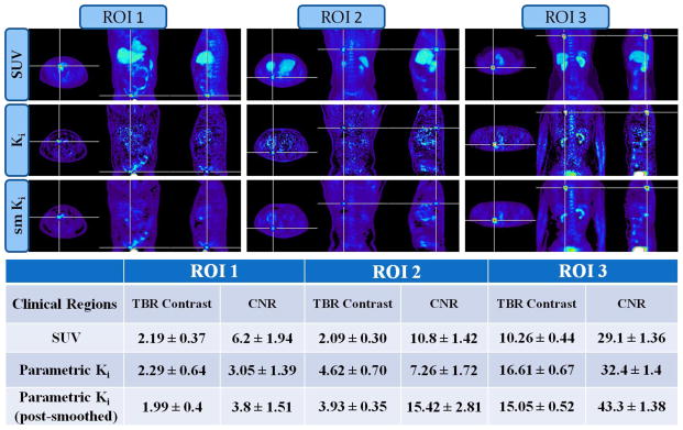
(top) Clinical whole-body SUV, Ki and post-smoothed Ki (sm Ki) images of three suspected tumor regions (bottom): tumor-to-background contrast values measured from extracted ROI mean values drawn on the previous images
5.2. Optimization of whole-body dynamic PET acquisition
True (noise-free) images and simulated frames acquired with protocol NP6_TF45 are illustrated in figure 9. The first row presents, from left to right, the true activity map of the last dynamic frame, the true parametric Ki image derived by performing Patlak fitting on the noise-free activity maps and a 3min frame, acquired 60min post injection, to approximate an SUV image. In the second and third row, they are displayed, from left to right, the last 6 dynamic frames acquired with GATE simulations and reconstructed with OSMAPOSL algorithm (21 subsets, 5 iterations).
Figure 9.

True (noise-free) and simulated PET cardiac bed frames acquired with protocol NP6_TF45: (1st row from left to right) The true activity map of the last frame (30th after including the first 24 cardiac frames), the true parametric Ki image and a simulated 3min SUV frame acquired from simulated data 60min post injection. (2nd and 3rd row from left to right) The last 6 simulated dynamic frames reconstructed with OS-MAP-OSL algorithm (21 subsets, 5 iterations)
The parametric Ki images produced by the set of acquisition schemes described in Table I are presented in figure 10. Figure 10a, from left to right and row by row, depicts the Ki images, as produced by sampling schemes with constant total study time (0–48min post injection) and variable number of passes (starting from 8 and decreasing to 2). The bed time frames increase proportionally as the number of passes decreases in order to keep the total acquisition shorter than 50min. The specific properties of this first set of examined protocols are presented in the left column of Table I. Similarly, figure 10b, from left to right and row by row, displays the Ki images as produced by schemes with constant 45sec bed time frames and variable number of passes starting from 6 and decreasing to 2. As a result. the total acquisition becomes shorter with decreasing number of passes (Table I, right column).
Figure 10.

Parametric Ki images produced by acquisition schemes of (a) From left to right, row by row: constant 45min total scan time and variable number of passes starting from 8 and decreasing to 2. (b) From left to right, row by row: constant 45sec bed time frames and variable number of passes starting from 6 and decreasing to 2.
Furthermore, in figures 11a and 11b the overall and ROI-based noise vs. bias curves are plotted together for the parametric images produced by the set of protocols with constant total study time of 45min. Similarly, figure 12 presents the respective curves for the parametric images generated from the set of protocols with constant time frames of 45sec and variable number of passes, ranging from 2 to 6. Each noise vs. bias plot consists of 10 points corresponding to parametric images derived from the first 10 OSEM full iterations of dynamic images.
Figure 11.
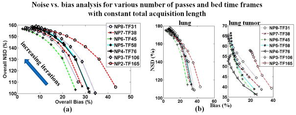
(a) Overall and (b) ROI-based noise vs. bias plots for parametric Ki images acquired according to protocols with a constant 50min total scan time post injection and variable number of passes and time frames. For all diagrams, proximity to the origin (i.e. low NSD and Bias) of a point or curve is a metric of good performance. The NSD values are increasing with increasing number of iterations (1 to 10).
Figure 12.
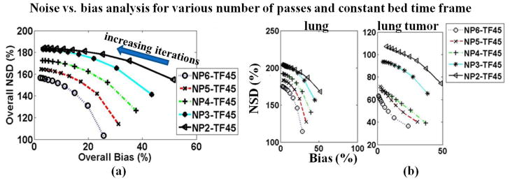
(a) Overall and (b) ROI-based noise vs. bias plots for parametric Ki images acquired with protocols of constant bed frame (45sec) and various number of passes ranging from 2 to 6. For all diagrams, proximity to the origin (i.e. low NSD and Bias) of a point or curve is a metric of good performance. The NSD values are increasing with increasing number of iterations.
5.3. Effect of WR-based thresholding and reduction of number of passes on whole-body Ki images
A range of WR reference values between 0.7 and 0.95 have been applied and for each the corresponding thresholded whole-body Ki image is produced both for clinical and simulated data, as it is shown in figures 13a and 13c respectively. The quantitative analysis on the simulated data in figure 13e indicates considerable CNR enhancement vs. SUV particularly when WR=0.9, suggesting this value as the optimal.
Figure 13.

(top row) Clinical whole-body Ki images, acquired with NP6_TF45 protocol, after (a) thresholding based on a range of different WR reference values and (b) gradually omitting the last dynamic frames of each bed. (middle row): (c) and (d) Same type of Ki images with top row, but for a simulated cardiac bed frame. (bottom row): Liver tumor CNR quantitative analysis for (e) large size tumor (liver) vs. WR threshold and (f) medium-sized tumor (liver2) vs. number of passes per bed. For the latter plot, the liver tumor CNR performance for protocols NP6_TF45, NP5_TF45 and NP3_TF45 was compared. The equivalent SUV images for the simulated and clinical data can be found at figures 9 and 7 respectively.
In addition, the last dynamic frames from each bed were gradually omitted from the parameter estimation process (in this study only OLS regression schemes are applied) to determine the effect of reduction of number of passes per bed on the resulting Ki images each time. The results in figure 13b for clinical and figure 13d for simulated Ki images, as well as the quantitative CNR analysis on simulated sata in figure 13f demonstrate the gradual degradation of CNR performance as the number of passes are reduced from six to three. However, Patlak OLS with just 4 passes per bed achieve equivalent CNR levels with SUV, while 5 and 6 passes per bed result in Ki images with superior tumor CNR.
The simulated data presented and analyzed in this section only originate from dynamic data produced with the second set of kinetic parameter values (Table II, right column). Moreover, the simulated activity maps employed in this section include 6 tumors, all located within a cardiac bed: 3 liver tumors designated as liver, liver2 and liver3 with 16mm, 12mm and 8mm diameter, respectively, and 3 lung tumors designated as lung, lung2 and lung3 of same sizes.
6. Discussion
6.1 Multi-bed dynamic acquisition protocols
6.1.1 Overlapped slices between adjacent beds
Whole-body PET acquisition systems usually overcome the relative low sensitivity of 3D bed acquisitions by overlapping the edge slices of each bed. Therefore, these overlapping planes contain data acquired at two different times. If access to the original bed data is not available, then an approach is needed to assign an effective time to the information for the data of the overlapped planes. In section 2.2.2 we proposed assigning the average of the mid-time points of the two adjacent beds to the overlapped planes between them. This method effectively introduces additional beds containing only the overlapped planes between adjacent beds.
The need for time averaging may be alleviated if the user has direct access to the original bed frame images before automatic overlap and averaging takes place. In this case, the original beds can be segmented into two or three new portions, each containing either the central or the edge planes of the original bed. Subsequently, voxel-wise Patlak can be applied to each of the new portions. Since the edge planes have been scanned twice at each pass, the dynamic frames of the beds composed of edge planes will be sampled twice as many times as the dynamic frames of the beds composed of central planes. At the same time, the edge planes suffer from higher statistical noise in each acquisition than the central planes, due to the relatively lower sensitivity of 3D bed acquisition in the edge planes. In addition, the time sampling for the edge planes will no longer be uniform. This is an interesting alternative approach worth further consideration and analysis, provided easy access to the original bed data is provided by the PET acquisition software.
6.1.2 Sequential dynamic scans for limited number of beds
An interesting study of glucose metabolism in adipose tissue by Ng et al. (2012) involved only 2 beds and proposing sequential dynamic scans across the beds, each lasting ~45min at the given bed position. However, this approach, (i) aside from having limited axial coverage, required (ii) a long total acquisition time with (iii) large time gaps for each bed, and (iv) arterial blood sampling to extract the input function. By contrast, our proposed protocol (i) enables whole-body imaging at (ii) reduced total scan times, with (iii) limited time acquisition gaps and (iv) non-invasive determination of the input function, by initially focusing on the heart and subsequently interleaving the dynamic acquisition evenly among multiple beds including the heart.
6.1.3 2D vs 3D acquisition mode
As we described earlier in section 2.2.1, our proposed protocol consists of an earlier phase of a 2D dynamic scan over the heart, followed by subsequent 3D whole body scans. When regions of very high activity are scanned, as is the case with the LV region in the early phase of our protocol, 2D acquisition mode can naturally help limiting the effects of dead-time randoms and scatter considerably and therefore increase the noise equivalent count rate (NECR) which can be considered an index of SNR or statistical quality in PET projection data (Strother et al 1990).
In fact for very high count rates, as is the case during the first phase of our proposed protocol, 2D acquisition mode can significantly limit the dead-time and randoms effects. As a result, the noise-equivalent count rate (NECR) rises and therefore the SNR and the statistical quality of the acquired projection data are enhanced with respect to 3D acquisitions for high count rates (Strother et al 1990). In terms of bias, 2D and 3D acquisitions are not expected to exhibit differences in performance assuming dead-time, randoms and scatter correction are performed accurately. The latter type of correction particularly needs attention as the reviewer raises: in fact, for scatter estimation and correction, the analytical deconvolution technique of Bergstrom et al (1983) was used for the 2D acquisition while for 3D mode a model-based algorithm was implemented by Iatrou et al (2004 and 2006) based on Ollinger’s (1996) and Wollenweber’s (2002) methods.
In the case of 2D acquisition the scatter fraction is considerably limited and the fast analytical method is considered adequate. However, for the 3D acquisition the scatter fraction becomes important and the scatter estimation and correction is a more challenging task. We make three observations regarding the quantitative comparison of 2D vs. 3D scattered corrected data. 1) An evaluation study by Spinks and Bastin (2008) have shown in cardiac studies that GE Discovery RX scatter correction method by Bergstorm et al (1983) in 2D mode is accurate and comparable with the method of Wollenweber (2002) in 3D, provided no excessive uptake is present adjacent to the region of interest in the case of 3D mode. However, Wollenweber method was later expanded by Iatrou et al (2006) to address the presence of high activity in neighboring regions and thus enhance quantitative accuracy. The latter scatter modeling method was incorporated in the 3D reconstruction software of GE Discovery RX based on the algorithm of Iatrou et al (2004). Moreover, (2) we have internally verified for this scanner with standardized cylindrical phantoms (20cm diameter and length) and for realistic count rates, that 2D and 3D measurements after scatter correction produce images that have an average difference of 0.5 ±1.2%, which made us comfortable with using this approach. Finally (3) our own figure 3a indicates a very smooth transition and no systematic discrepancies between the section of the input function curve corresponding to the initial 2D phase (0–6min) and the remaining later section belonging to the later 3D acquisition phase. However, we should also note that for other type of scanners, regions and correction algorithms 2D and 3D data may not be quantitatively similar and, thus, a literature review as well as a phantom evaluation study is highly necessary, before applying the proposed protocol.
6.2 Parametric vs. SUV PET imaging comparison
By examining the patient studies and simulated scans in the current study, the tumor-to-background contrast environments may be classified into three characteristic categories, commonly found in FDG PET oncology studies:
high uptake rate tumors surrounded by high, but constant, background activity (e.g. simulated liver tumor in section 4.1 and figures 6, 9 and 10),
low uptake rate tumors surrounded by low background activity (e.g. simulated lung tumor in section 4.1 and figures 6, 9 and 10), and
high uptake rate tumors surrounded by low uptake background, such as the distinct lung tumor observed in one of the patient FDG studies (section 5.1, figure 7, figure 8 ROI 3).
For the first class of contrast environments, the results show better CNR performance, relative to SUV, for the proposed whole-body Patlak OLS Ki imaging framework, as it effectively removes the background activity regions. On the other hand, for the second type of contrast regions, the results indicate better CNR for SUV. We attribute this to the high levels of noise in the parametric image voxels as a result of the low activity levels in tumor regions as well as the short dynamic PET frames. Moreover, an additional factor that may have contributed to the lower CNR for this case is the reversible kinetics with which our simulated lung tumor is associated. As we have demonstrated in a recent study (Karakatsanis et al 2013c), Patlak standard model may underestimate Ki, and, thus, tumor Ki contrast, in certain regions characterized by non-negligible dephosphorylation rates k4 (i.e. reversibility), as is the case here with the simulated lung tumor region in section 4.1 (also see k4 value for lung tumor in right section of Table II). Finally, for the third class of contrast environments, both SUV and parametric OLS imaging perform comparably, with the latter having a small advantage which becomes significant after post-smoothing, as our clinical results demonstrate (figure 7, figure 8 ROI 3).
Therefore, when the observer task involves tumor detectability, we propose complementary application of parametric imaging, along with SUV, to benefit from the advantages of both techniques in all regions across the whole body. An interesting research direction we are pursuing involves dynamic whole-body imaging in the 60–90min post-injection interval, enabling simultaneous SUV and Ki parametric imaging from a single dataset, though this approach would require the use of population based input function estimation methods (as the blood pool will only be sampled at later times).
6.3 Whole-body Patlak Ki vs other simplified Ki estimation methods
In the past, quantitative yet simplified FDG metabolic rate estimation methods have been proposed, involving a single PET scan 45min to 1hr post-injection and a complete input function. The tracer retention method (Hunter et al 1996), suggests as a metric for the metabolic glucose rate the tracer activity concentration, measured from a static scan, divided by the integral of the input function from injection to scan time, also known as the fractional uptake ratio (FUR). For this simplification, the method effectively assumes VCp(t) is negligible with respect to C(t) in equation 2, which may not be valid especially at earlier times and in low uptake regions, thus challenging accurate quantification. Also this metric is time-dependent as the relative accuracy of assuming VCp(t) is negligible depends on time. In tumor imaging, the authors did observe good correlation of their results with Ki estimates derived from a fit to a two-tissue compartment model. However, this correlation is time- and tumor-dependent as explained above.
Another simplified quantitative method developed in the past is the autoradiographic method as first introduced by Sokoloff et al (1977) for non-gamma emitters in rats and later adjusted for human brain FDG studies by Huang et al (1980). Similarly it involves a single scan 1hr post injection and a complete input function. In addition, a set of pre-determined rate constants K1, k2, k3 and k4 of the two-tissue compartmental model is required, which can be derived from mean values of a reference population. It was recently demonstrated in a review by Galli et al (2013) that the accuracy of the autoradiographic method relies on the assumption that the free (non-phosporylated) amount of glucose tracer left in the tissue at the time of scan is negligible to the bound or phosphorylated amount. Even then, the contribution of blood volume to tissue activity may still render the autoradiographic method relatively inaccurate. A recent evaluation of the method by Burger et al (2011) employing this technique demonstrated high correlation between the autoradiographically estimated Ki and Patlak Ki imaging, the latter considered the golden standard. They also showed that time-dependence of the metric was diminished with respect to SUV imaging, but still considerable with respect to Patlak Ki imaging.
Moreover, the two simplified techniques are challenged by the fact that while they only need a single static scan, they require a complete input function, which cannot be derived from the single scan data, and therefore, may require invasive sampling. By contrast, our proposed dynamic multi-bed protocol including Patlak modeling enables non-invasive, image-driven characterization of the input function.
6.4 Selection of the Patlak kinetic correlation-coefficient (WR) reference value
The performance of WR driven thresholding is largely affected by the selection of the WR reference or threshold value. Assuming that the kinetic correlation coefficient WR quantifies the voxel TACs statistical quality, our aim is to determine the optimal WR reference value such as the resulting two WR clusters (high- and low-WR clusters) best classifies the voxel TACs of the dynamic image set into those of high and those of low statistical quality. However, each observer task may have different objectives and may employ different criteria when considering a certain voxel TAC as of high or low statistical quality. As a result, the optimal WR threshold is task dependent. In addition, the optimal WR reference can be patient- and region-dependent as it may be affected by the particular noise levels present in each tumor region, which may differ among the various contrast environments and across members of patients population. Thus, the optimal WR threshold may also be patient- as well as region-specific. Overall, the free nature of the kinetic correlation parameter provides the proposed whole body PET parametric imaging framework with flexible task-based strategies, as elaborated further in our companion paper (Karakatsanis et al 2013b).
For the range of contrast regions studied, both in our realistic simulations and the patient data, and for the average noise levels associated with the short bed frames (45sec) of the optimal NP6_TF45 protocol, we have identified that a range of WR reference values between 0.6 and 0.95 should be initially examined. Within that range, the value yielding optimal task performance should be selected. In the context of treatment response monitoring, application of low WR reference values implies mild thresholding retaining high quantification at the cost of relatively lower CNR. On the other hand, in the context of diagnosis and tumor detectability where the aim is CNR enhancement, relatively higher WR reference values can be selected, at the potential cost of compromising quantification in the parameter estimates or even lesion detection, if the WR reference is set very close to unity. Therefore, it is critical, for the clinical adoption of the proposed method, to initially define an optimal range with an upper limit that ensures no significant degradation of tumor quantification or CNR and within which the optimal WR reference can be freely adjusted according to the specific task objectives.
6.5 Future prospects
6.5.1 PET/MR imaging
In the context of PET/MR imaging, the relatively increased time associated with multi-bed dynamic PET acquisitions can enable simultaneous multiple MR sequences (Judenhofer et al 2008), which usually also require lengthy acquisitions, to provide a wealth of multi-modality information, including but not limited to radiation-free high resolution anatomical maps (Seemann et al 2005, Hoffmann et al 2009). Although the optimum way to deploy the technology is still under development (Catana et al 2013), a range of different MR sequences are available, including T1-, T2-, diffusion-weighted and dynamic contrast-enhanced MR imaging (Moser et al 2009). Whereas much PET/CT protocol development has been aimed at reducing PET acquisition times (Halpern et al 2004, Karakatsanis et al 2009), with simultaneous PET/MR, overall scan durations are expected to be longer to enable multiple MR sequences and provide a significant opportunity for innovative PET acquisitions and enhanced whole-body PET quantification.
6.5.2 Treatment response monitoring
The proposed methodology is particularly significant for treatment response monitoring, because:
the tracer uptake rate Ki is a more quantitative estimate than SUV and, when utilized in the whole-body domain, may enable truly quantitative and time independent assessment of the treatment effect on the localized and metastatic progress of cancer and,
the suppressed tumor uptake can be differentiated from the background in the challenging post-treatment setting particularly in regions where the tumor exhibits non-negligible uptake, even after treatment, and is surrounded by relatively high background (e.g. liver tumors). The parametric Ki values in background regions of relatively constant but high activity have been shown to approach “zero” unlike background SUV values (Zasadny and Wahl 1993), resulting in enhanced tumor contrast in Ki images.
The quantitative accuracy, as presented in the first point above, is very important when assessing treatment response from a series of imaging studies conducted throughout a large period, as it ensures quantitative comparisons between a range of whole-body PET scans. Furthermore, the contrast enhancement capabilities, as presented in at the second point above, are particularly important especially in the case of post-treatment PET scans, where the uptake in tumors may be suppressed after therapy and, thus, neglected in SUV scans if comparable with background activity. Thus, we believe that the new method combining quantitative and contrast-enhanced whole-body imaging may significantly impact clinical oncology PET.
6.5.3 Motion and partial volume effects in whole-body Ki imaging
Patient movements can challenge oncological whole-body PET imaging as they cause smearing artifacts of active tumor and background structures, resulting in CNR and quantification errors (Dinges et al 2013). Although periodic motion-induced artifacts can be limited with gated acquisition (Nehmeh et al 2013, Nekolla et al 2013) and advanced 4D image reconstruction (Rahmim et al 2013), many other types of patient motion are irregular, involuntary and more likely to occur during long dynamic PET acquisitions and at random time points (Dinges et al 2013). The length of the acquisition as well as the voxel-based parameter estimation process involved in our proposed whole-body PET parametric imaging framework may increase the presence of motion artifacts and their propagation to the parametric image domain. On the other hand, partial volume effects (PVE), which may also induce bias and loss of CNR in tumor imaging (Rousset et al 2007, Soret et al 2007, Erlandsson et al 2012), produce a similar impact in both SUV and Ki imaging (Freedman et al 2003).
The kinetic correlation parameter could be utilized as an indicator for the presence of motion or partial volume effect in each voxel TAC. Assuming relative uniformity in tumor and other regions, motion is expected to exercise larger impact on voxels situated at the boundaries between two regions, therefore the WR correlation of these voxel TACs is expected to decrease with higher extent of motion. In addition, PVE may affect certain voxel TACs at the boundaries of regions characterized by different uptake rates, also resulting in WR reduction. Therefore, by applying WR-based thresholding, motion contaminated or PVE affected voxel TACs at the boundaries of tumors or other regions could effectively be filtered out from the parameter estimation process. If the regions are relatively uniform, motion and, thus, zero-thresholding will only affect the region boundaries. However, in cases of non-uniform regions (e.g. when tumor exhibits non-uniform uptake), extensive thresholding may result in filtering out of voxels within the regions of interest as well, thus, inducing noise and quantification errors. Therefore, the WR threshold should be selected with caution avoiding very large values (i.e. close to unity) as they may give rise to artifacts in regions affected by motion or PVE.
In the current clinical study, CNR increases in Ki images when applying WR thresholding, mainly because the noise is reduced in the background. Moreover, qualitative inspection of the clinical images (figure 13) shows that the smearing artifact in the tumor regions is limited after thresholding, indicating lower WR correlation in tumor boundaries potentially because of respiratory motion (lung tumor). Therefore, we attribute the reduction of smearing effect to the thresholding of motion- and PVE-affected voxels present in whole-body dynamic data.
6.5.4 Applicability to other tracers
For simulated and clinical assessment of our imaging framework, as previously introduced in conference proceedings (Karakatsanis et al 2011, 2012a and 2012b), the 18F-fluoro-deoxy-glucose (FDG) tracer was selected due to its wide and established application scope both in dynamic and whole-body PET oncology studies. However, the proposed framework can be applicable to a host of other tracers satisfying the Patlak model assumptions, within reasonable accuracy, as described in section 2.1. Recently, another study was reported (Guo et al 2012) involving a clinical application of whole-body PET parametric imaging using 68Ga-NOTA-PRGD2 on lung cancer patients, indicating a potentially growing interest in the PET community towards dynamic whole-body imaging.
7. Summary and Conclusions
In the current study we a) propose and optimize a novel clinically feasible 4D whole-body PET acquisition protocol and, subsequently, b) enhance it with statistically adaptive image thresholding, by efficiently utilizing Patlak kinetic correlation information, as extracted from 4D acquired data. Our aim is to present an integrated imaging framework capable of triggering a novel shift of clinical whole-body PET imaging to the dynamic domain, potentially enabling tumor contrast enhancements, while allowing quantitative whole-body assessment of patient response to treatments over short and long time periods.
The proposed whole body PET parametric imaging framework, as demonstrated by both clinical and simulated results, is clinically feasible and capable of delivering quantitative estimates of tracer metabolic uptake rate Ki across multiple beds. Furthermore, it has the potential to achieve considerably higher CNR than SUV, particularly in tumor regions with high uptake rate surrounded by background regions of high but constant activity, such as the liver.
The effective removal of large background regions, exhibiting high non-malignant uptake in SUV images (e.g. kidneys and liver), from whole-body parametric images constitutes a major benefit for the proposed methods. The comparative evaluation of SUV and Ki whole-body images has demonstrated that translating from SUV to standard OLS Patlak has the potential to dramatically enhance tumor CNR. Further enhancements in specific contrast environments may be possible with the introduction of more advanced Patlak schemes, as we show in the companion study (Karakatsanis et al 2013b).
The presented multi-bed dynamic PET acquisition protocol is streamlined for clinical adoption, as it involves simple uni-directional scanning and equal bed frame durations. Owing to its ability to efficiently combine estimation of the blood input function with acquisition of tissue time activity concentrations, not only at the ROI but also at the voxel level, it allows for whole-body parametric Patlak imaging. The comparative evaluation of the produced Ki images for different protocols (figure 11) suggested NP6_TF45 as the optimal acquisition scheme. Moreover, the number of passes per bed and, thus, the total acquisition time can be reduced to five passes (~40min) and still obtain higher CNR than SUV (figure 12). Even with four passes (total length: ~35min) the two CNR values are equivalent.
The current study involves indirect estimation of parametric images from OSEM reconstructed dynamic whole-body FDG images, acquired over a period of 30–45min post injection, employing the standard Patlak linear model. As future work, we are investigating (Karakatsanis et al 2013a) the extension of the proposed framework to the direct 4D parametric image reconstruction domain (Wang et al 2008, Tsoumpas et al 2008, Tang et al 2010, Wang and Qi 2010) to directly estimate the parametric images from the dynamic sinogram data in order to further limit the noise in the estimates induced by the limited scan time of each bed dynamic frame.
Moreover, the current evolution trend of modern whole-body PET/CT and PET/MR imaging systems towards increasing axial bed lengths and higher detection efficiencies can only have a positive impact on the feasibility and acceptance of the presented whole-body parametric PET imaging framework, as it will allow for multi-bed dynamic acquisitions of higher statistical quality in shorter periods of time over less bed positions (though same total axial coverage), further accelerating the clinical adoption of the proposed methods.
Acknowledgments
The authors would like to thank Dr William P. Segars and the openGATE collaboration for providing us with the XCAT phantom and the GATE software, respectively. Furthermore, we would also like to acknowledge Dr Joyce Mhlanga and John Crandall for assistance in recruiting patients for our clinical studies, Andy Crabb for computational support, and Hassan Mohy-ud-Din for helpful discussions. This work was in part supported by the NIH grant 1S10RR023623.
References
- Adams M, Turkington T, Wilson J, Wong T. A systematic review of the factors affecting accuracy of SUV measurements. American Journal of Roentgenology. 2010;195(2):310–320. doi: 10.2214/AJR.10.4923. [DOI] [PubMed] [Google Scholar]
- Allen D. Mean Square Error of Prediction as a Criterion for Selecting Variables. Technometrics. 1971;13(3):469–475. [Google Scholar]
- Bergstorm M, Eriksson L, Bohn C, Blomqvist G, Litton J. Correction for scattered radiation in a ring detector positron camera by integral transformation of the projections. J Comput Assist Tomogr. 1983;7:42–50. doi: 10.1097/00004728-198302000-00008. [DOI] [PubMed] [Google Scholar]
- Burger I, Burger C, Berthold T, Buck A. Simplified quantification of FDG metabolism in tumors using the autoradiographic method is less dependent on the acquisition time than SUV. Nuclear Medicine and Biology. 2011;38:835–841. doi: 10.1016/j.nucmedbio.2011.02.003. [DOI] [PubMed] [Google Scholar]
- Castell F, Cook G. Quantitative techniques in 18-FDG PET scanning in oncology. British Journal of Cancer. 2008;98(10):1597–1601. doi: 10.1038/sj.bjc.6604330. [DOI] [PMC free article] [PubMed] [Google Scholar]
- Catana C, Guimaraes AR, Rosen BR. PET and MR Imaging: The Odd Couple or a Match Made in Heaven. J Nucl Med. 2013;54:815–824. doi: 10.2967/jnumed.112.112771. [DOI] [PMC free article] [PubMed] [Google Scholar]
- Dahlbom M, Hoffman E, Hoh C, Schiepers C, Rosenqvist G, Hawkins R, Phelps M. Whole-body positron emission tomography: Part i. methods and performance characteristics. J of Nucl Med. 1992;33(6):1191. [PubMed] [Google Scholar]
- Dimitrakopoulou-Strauss A, Georgoulias V, Eisenhut M, Herth F, Koukouraki S, Macke H, Haberkorn U, Strauss L. Quantitative assessment of SSTR2 expression in patients with non-small cell lung cancer using 68 Ga-DOTATOC PET and comparison with 18 F-FDG PET. Eur J Nucl Med and Mol Imaging. 2006;33(7):823–830. doi: 10.1007/s00259-005-0063-5. [DOI] [PubMed] [Google Scholar]
- Dimitrakopoulou-Strauss A, Strauss L, Burger C. Quantitative PET studies in pretreated melanoma patients: a comparison of 6-[18F] fluoro-L-dopa with 18F-FDG and 15O-water using compartment and noncompartment analysis. J Nucl Med. 2001;42(2):248–256. [PubMed] [Google Scholar]
- Dimitrakopoulou-Strauss A, Strauss L, Burger C, Ruhl A, Irngartinger G, Stremmel W, Rudi J. Prognostic aspects of 18F-FDG PET kinetics in patients with metastatic colorectal carcinoma receiving FOLFOX chemotherapy. J Nucl Med. 2004;45(9):1480–1487. [PubMed] [Google Scholar]
- Dimitrakopoulou-Strauss A, Strauss L, Schwarzbach M, Burger C, Heichel T, Willeke F, Mechtersheimer G, Lehnert T. Dynamic PET 18F-FDG studies in patients with primary and recurrent soft-tissue sarcomas: impact on diagnosis and correlation with grading. J of Nucl Med. 2001;42(5):713–720. [PubMed] [Google Scholar]
- Dimitrakopoulou-Strauss A, Strauss L, Schwarzbach M, Burger C, Heichel T, Willeke F, Mechtersheimer G, Lehnert T. Dynamic PET 18F-FDG studies in patients with primary and recurrent soft-tissue sarcomas: impact on diagnosis and correlation with grading. J Nucl Med. 2001;42(5):713–720. [PubMed] [Google Scholar]
- Dinges J, Nekolla SG, Bundschuh RA. Motion artifacts in oncological and cardiac PET imaging. PET Clin. 2013;8:1–9. doi: 10.1016/j.cpet.2012.10.001. [DOI] [PubMed] [Google Scholar]
- Effron B, Tibshirani RJ. CRC, editor. An introduction to the Bootstrap. New York: Chapman Hall; 1993. [Google Scholar]
- Erlandsson K, Buvat I, Pretorius PH, Thomas BA, Hutton BF. A review of partial volume correction techniques for emission tomography and their applications in neurology, cardiology and oncology. Phys Med Biol. 2012;57(2012):R119–R159. doi: 10.1088/0031-9155/57/21/R119. [DOI] [PubMed] [Google Scholar]
- Facey K, Bradbury I, Laking G, Payne E. Overview of the clinical effectiveness of positron emission tomography imaging in selected cancers. Health Technology Assessment. 2007;11(44) doi: 10.3310/hta11440. [DOI] [PubMed] [Google Scholar]
- Freedman NM, Sundaram SK, Kurdziel K, Carrasquillo JA, Whatley M, Carson JM, Sellers D, Libutti SK, Yang JC, Bacharach SL. Comparison of SUV and Patlak slope for monitoring of cancer therapy using serial PET scans. Eur J Nucl Med Mol Imag. 2003;30(1) doi: 10.1007/s00259-002-0981-4. [DOI] [PubMed] [Google Scholar]
- Galli G, Indovina L, Calcagni ML, Mansi L, Giordano A. The quantification with FDG as seen by a physician. Nuclear Medicine and Biology. 2013;40:720–730. doi: 10.1016/j.nucmedbio.2013.06.009. [DOI] [PubMed] [Google Scholar]
- Gonias P, Bertsekas N, Karakatsanis N, Saatsakis G, Nikolopoulos D, Tsantilas X, Loudos G, Sakellios N, Gaitanis A, Papaspyrou L, Daskalakis A, Liaparinos P, Cavouras D, Kandarakis I, Panyiotakis G. Validation of a GATE Model for the simulation of the Siemens PET/CT Biograph 6 Scanner. Nuclear Instruments and Methods in Physics Research Section A. 2007;569(2):368–372. [Google Scholar]
- Guo N, Zhu Z, Zheng K, Xing H, Li F, Chen X, Li Q. Multi-bed position dynamic imaging and kinetic analysis of 68Ga-NOTA-PRGD2 in lung cancer patients. J Nucl Med. 2012;53(Supplement 1):1253. [Google Scholar]
- Halpern BS, Dahlbom M, Quon A, Schiepers C, Waldherr C, Silverman DH, Ratib O, Czernin J. J Nucl Med. 2004;45(5):797–801. [PubMed] [Google Scholar]
- Hamberg L, Hunter G, Alpert N, Choi N, Babich J, Fischman A. The dose uptake ratio as an index of glucose metabolism: Useful parameter or oversimplification? J of Nucl Med. 1994;35(8):1308. [PubMed] [Google Scholar]
- Haynor DR, Woods SD. Resampling estimates of precision in emission tomography. IEEE Trans Med Imag. 1989;8(4):337–343. doi: 10.1109/42.41486. [DOI] [PubMed] [Google Scholar]
- Hofmann M, Pichler B, Scholkopf B, Beyer T. Towards Quantitative PET/MRI: A review of MR-based attenuation correction techniques. Eur J Nucl Med Mol Imaging. 2009;36(Suppl 1):S93–104. doi: 10.1007/s00259-008-1007-7. [DOI] [PubMed] [Google Scholar]
- Ho-Shon K, Feng D, Hawkins AR, Meikle S, Fulham M, Li X. Optimized Sampling and Parameter Estimation for Quantification in Whole Body PET. IEEE Trans on Biom Eng. 1996;43(10) doi: 10.1109/10.536903. [DOI] [PubMed] [Google Scholar]
- Huang S. Anatomy of SUV. Nucl Med and Biol. 2000;27(7):643–646. doi: 10.1016/s0969-8051(00)00155-4. [DOI] [PubMed] [Google Scholar]
- Huang S, Phelps ME, Hoffman EJ, Sideris K, Selin C, Kuhl DE. Nonivasive determination of local cerebral metabolic rate of glucose in man. Am J Physiol Endocrinol Metab. 1980;238:E69–E82. doi: 10.1152/ajpendo.1980.238.1.E69. [DOI] [PubMed] [Google Scholar]
- Hunter GJ, Hamberg LM, Alpert NM, Choi NC, Fischman AJ. Simplified measurement of deoxyglucose utilization rate. J Nucl Med. 1996;37(6) [PubMed] [Google Scholar]
- Hustinx R, Benard F, Alavi A. Whole-body FDG-PET imaging in the management of patients with cancer. Seminars in nuclear medicine. 2002;32(1):35–46. doi: 10.1053/snuc.2002.29272. [DOI] [PubMed] [Google Scholar]
- Iatrou M, Manjeshwar RM, Ross SG, Thielemans K, Stearns CW. 3D implementation of scatter estimation in 3D PET. IEEE Nucl Sci Symposium Conf Record. 2006;M06–332 [Google Scholar]
- Iatrou M, Ross SG, Manjeshwar RM, Stearns CW. A fully 3D iterative image reconstruction algorithm incorporating data corrections. IEEE Nucl Sci Symposium Conf Record. 2004:2493–2497. [Google Scholar]
- Jan S, et al. GATE V6: a major enhancement of the GATE simulation platform enabling modeling of CT and radiotherapy. Phys Med Biol. 2011;56:881. doi: 10.1088/0031-9155/56/4/001. [DOI] [PubMed] [Google Scholar]
- Judenhofer MS, Wehrl HF, Newport DF, Catana C, Siegel SB, Becker M, Thielscher A, Kneilling M, Lichy M, Eichner M, Klingel K, Reischi G, Wildmaier S, Rocken M, Nutt RE, Machulla HJ, Kamil U, Cherry SR, Claussen CD, Pichler BJ. Simultaneous PET-MRI: a new approach for functional and morphological imaging. Nature Medicine. 2008;14:459–465. doi: 10.1038/nm1700. (2008) [DOI] [PubMed] [Google Scholar]
- Kaneta T, Takai Y, Iwata R, Hakamatsuka T, Yasuda H, Nakayama K, Ishikawa Y, Watanuki S, Furumoto S, Funaki Y, Nakata E, Jingu K, Tsujitani M, Masatoshi I, Fukuda H, Takahashi S, Yamada S. Initial evaluation of dynamic human imaging using 18F-FRP170 as a new PET tracer for imaging hypoxia. Ann of Nucl Med. 2007;21(2):101–107. doi: 10.1007/BF03033987. [DOI] [PubMed] [Google Scholar]
- Karakatsanis N, Lodge M, Mohy-ud-Din H, Tahari A, Zhou Y, Segars W, Wahl R, Rahmim A. Enhanced Whole-Body PET Parametric Imaging Using Hybrid Regression and Thresholding Driven by Kinetic Correlations. IEEE Nucl Sci Symp and Med Imaging Conf Record 2012b [Google Scholar]
- Karakatsanis N, Lodge M, Tahari AK, Zhou Y, Wahl RL, Rahmim A. Dynamic whole body PET parametric imaging: I. Concept, acquisition protocol optimization and clinical application. Phys in Med and Biology. 2013b doi: 10.1088/0031-9155/58/20/7391. [DOI] [PMC free article] [PubMed] [Google Scholar]
- Karakatsanis N, Lodge M, Wahl RL, Rahmim A. Direct 4D whole-body PET/CT parametric image reconstruction: Concept and comparison vs. indirect parametric imaging. J Nucl Med 2013. 2013a;54(Supplement 2):2133. [Google Scholar]
- Karakatsanis N, Lodge M, Zhou Y, Mhlanga J, Tahari A, Chaudhry M, Segars W, Wahl R, Rahmim A. Dynamic Multi-Bed FDG PET imaging: Feasibility and optimization. IEEE Nucl Sci Symp and Med Imaging Conf Record 2011 [Google Scholar]
- Karakatsanis N, Lodge M, Zhou Y, Mhlanga J, Tahari A, Wahl R, Rahmim A. Towards Parametric Whole-Body FDG PET/CT Imaging: Potentials for Enhanced Tumor Detectability. J Nucl Med. 2012a;53(suppl 1):1236. [Google Scholar]
- Karakatsanis N, Loudos G, Nikita K. A Methodology for Optimizing the Acquisition Time of a Clinical PET Scan Using GATE. IEEE Nucl Sci Symp and Med Imaging Conf Record 2009 [Google Scholar]
- Karakatsanis N, Sakellios N, Tsantilas X, Dikaios N, Tsoumpas C, Nikita K, Lazaro D, Loudos G, Louizi A, Valais I, Nikolopoulos D, Malamitsi J, Kandarakis I. A Comparative Evaluation of Two Commercial PET Scanners using GATE. Nuclear Instruments and Methods in Physics Research Section A. 2006;569(2):368–372. [Google Scholar]
- Karakatsanis N, Zhou Y, Lodge M, Casey ME, Wahl RL, Rahmim A. Quantitative Whole-Body Parametric PET Imaging Incorporating a Generalized Patlak Model. IEEE Nucl Sci Symp and Med Imaging Conf Record 2013c [Google Scholar]
- Keyes J., Jr SUV: Standard uptake or silly useless value? J of Nucl Med. 1995;36(10):1836. [PubMed] [Google Scholar]
- Kim C, Gupta N. Dependency of standardized uptake values of fluorine-18 fluorodeoxyglucose on body size: comparison of body surface area correction and lean body mass correction. Nuclear medicine communications. 1996;17(10):890. doi: 10.1097/00006231-199610000-00011. [DOI] [PubMed] [Google Scholar]
- Kim C, Gupta N, Chandramouli B, Alavi A. Standardized uptake values of FDG: body surface area correction is preferable to body weight correction. J of Nucl Med. 1994;35(1):164. [PubMed] [Google Scholar]
- Kubota K, Itoh M, Ozaki K, Ono S, Tashiro M, Yamaguchi K, Akaizawa T, Yamada K, Fukuda H. Advantage of delayed wholebody FDG-PET imaging for tumour detection. Eur J of Nucl Med and Mol Imaging. 2001;28(6):696–703. doi: 10.1007/s002590100537. [DOI] [PubMed] [Google Scholar]
- Leskinen-Kallio S, Nagren K, Lehikoinen P, Ruotsalainen U, Teras M, Joensuu H. Carbon-11-methionine and PET is an effective method to image head and neck cancer. k. J of Nucl Med. 1992;33(5):691. [PubMed] [Google Scholar]
- Moser E, Stadlbauer A, Windischberger C, Quick H, Ladd ME. Magnetic Resonance imaging methodology. Eur J Nucl Med Mol Imaging. 2008;36(Suppl 1):S30–S41. doi: 10.1007/s00259-008-0938-3. [DOI] [PubMed] [Google Scholar]
- Nakamoto Y, Chin BB, Cohade C, Osman M, Tatsumi M, Wahl RL. Nuc Med Commun. 2004;25(3):221–5. doi: 10.1097/00006231-200403000-00002. [DOI] [PubMed] [Google Scholar]
- Nehmeh SA. Respiratory motion correction strategies in thoracic PET-CT imaging. PET Clin. 2013;8:29–36. doi: 10.1016/j.cpet.2012.10.004. [DOI] [PubMed] [Google Scholar]
- Nekolla SG, Dinges J, Rischpler C. Clinical impact of cardiac-gated PET imaging. PET Clin. 2013;8:69–79. doi: 10.1016/j.cpet.2012.10.002. [DOI] [PubMed] [Google Scholar]
- Ng J, Azuma K, Kelley C, Pencek R, Radikova Z, Laymon C, Price J, Goodpaster B, Kelley D. Am J Physiol Endocrinal Metab. 2012;303:E1134–E1141. doi: 10.1152/ajpendo.00282.2012. [DOI] [PMC free article] [PubMed] [Google Scholar]
- Okazumi S, Dimitrakopoulou-Strauss A, Schwarzbach M, Strauss L. Quantitative, dynamic 18F-FDG-PET for the evaluation of soft tissue sarcomas: relation to differential diagnosis, tumor grading and prediction of prognosis. Hel J Nucl Med. 2009;12(3):223. [PubMed] [Google Scholar]
- Ollinger JM. Model-based scatter correction for fully 3D PET. Phys Med Biol. 1996;41:153–176. doi: 10.1088/0031-9155/41/1/012. [DOI] [PubMed] [Google Scholar]
- Patlak C, Blasberg R. Graphical evaluation of blood-to-brain transfer constants from multiple-time uptake data. Generalizations. J of Cereb Blood Flow Metab. 1985;5(4):584–590. doi: 10.1038/jcbfm.1985.87. [DOI] [PubMed] [Google Scholar]
- Patlak C, Blasberg R, Fenstermacher J. Graphical evaluation of blood-to-brain transfer constants from multiple-time uptake data. J Cereb Blood Flow Metab. 1983;3(1):1–7. doi: 10.1038/jcbfm.1983.1. [DOI] [PubMed] [Google Scholar]
- Pichler BJ, Kolb A, Nagele T, Schlemmer HP. PET/MRI: Paving the way for the next generation of clinical multimodality imaging applications. J Nucl Med. 2010;51(3):383–336. doi: 10.2967/jnumed.109.061853. [DOI] [PubMed] [Google Scholar]
- Qiao H, Bai J, Chen Y, Tian J. Kidney Modeling for FDG Excretion with PET. Int J of Biom Imaging. 2007;2007:632–634. doi: 10.1155/2007/63234. [DOI] [PMC free article] [PubMed] [Google Scholar]
- Rahmim A, Tang J, Zaidi H. Four-dimensional image reconstruction strategies in cardiac-gated and respiratory-gated PET imaging. PET Clin. 2013;8:51–67. doi: 10.1016/j.cpet.2012.10.005. [DOI] [PubMed] [Google Scholar]
- Rousset O, Rahmim A, Alavi A, Zaidi H. Partial volume correction startegies in PET. PET Clin. 2007;2(2):235–249. doi: 10.1016/j.cpet.2007.10.005. [DOI] [PubMed] [Google Scholar]
- Sadato N, Tsuchida T, Nakaumra S, Waki A, Uematsu H, Takahashi N, Hayashi N, Yonekura Y, Ishii Y. Non-invasive estimation of the net influx constant using the standardized uptake value for quantification of FDG uptake of tumours. Eur J of Nucl Med and Mol Imaging. 1998;25(6):559–564. doi: 10.1007/s002590050256. [DOI] [PubMed] [Google Scholar]
- Sakellios N, Rubio JL, Karakatsanis N, Kontaxakis G, Loudos G, Santos A, Nikita KS, Majewski S. GATE simulations for small animal SPECT/PET using voxelized phantoms and rotating-head detectors. IEEE Nucl Sci Symp and Med Imag Conf. 2006;4 [Google Scholar]
- Seemann MD. Whole-body PET/MRI: The Future in Oncological Imaging. Technology in Cancer Research and Treatment. 2005;4(5):577–582. doi: 10.1177/153303460500400512. [DOI] [PubMed] [Google Scholar]
- Segars W, Sturgeon G, Mendonca S, Grimes J, Tsui B. 4D XCAT phantom for multimodality imaging research. J Medical Physics. 2010;37:4902. doi: 10.1118/1.3480985. [DOI] [PMC free article] [PubMed] [Google Scholar]
- Sokoloff L, Reivich M, Kennedy C, Des Rosiers MH, Patlak CS, Pettigrew KD, Sakurada O, Shinohara M. The (C-14) deoxyglucose method for the measurement of local cerebral glucose utilization: theory, procedure and normal values in the conscious and anesthetized albino rat. J Neurochem. 1977;28:897–916. doi: 10.1111/j.1471-4159.1977.tb10649.x. [DOI] [PubMed] [Google Scholar]
- Soret M, Bacharach S, Buvat I. Partial volume effect in PET tumor imaging. J Nucl Med. 2007;48(6):932–945. doi: 10.2967/jnumed.106.035774. [DOI] [PubMed] [Google Scholar]
- Spinks TJ, Bastin JE. Quantitative accuracy in cardiac studies with the GE Discovery RX PET/CT Scanner. IEEE Nuclear Science Symposium Conference Record. 2008;M06–9:3697–3701. [Google Scholar]
- Strauss L, Klippel S, Pan L, Schonleben K, Haberkorn U, Dimitrakopoulou-Strauss A. Assessment of quantitative FDG PET data in primary colorectal tumors: which parameters are important with respect to tumor detection? Eur J Nucl Med and Mol Imaging. 2007;34(6):868–877. doi: 10.1007/s00259-006-0319-8. [DOI] [PubMed] [Google Scholar]
- Strauss L, Koczan D, Klippel S, Pan L, Cheng C, Willis S, Haberkorn U, Dimitrakopoulou-Strauss A Impact of angiogenesis-related gene expression on the tracer kinetics of 18F-FDG in colorectal tumors. J Nucl Med. 2008;49(8):1238–1244. doi: 10.2967/jnumed.108.051599. [DOI] [PubMed] [Google Scholar]
- Strother SC, Casey ME, Hoffman EJ. Measuring PET scanner sensitivity: relating countrates to image signal-to-noise ratios using equivalents counts. IEEE Transac Nuclear Science. 1990;37(2):783–788. [Google Scholar]
- Sugawara Y, Zasadny K, Grossman H, Francis I, Clarke M, Wahl R. Germ cell tumor: Differentiation of viable tumor, mature teratoma, and necrotic tissue with FDG PET and kinetic modeling. Radiology. 1999;211(1):249–256. doi: 10.1148/radiology.211.1.r99ap16249. [DOI] [PubMed] [Google Scholar]
- Tang J, Kuwabara H, Wong DF, Rahmim A. Direct 4D reconstruction of parametric images incorporating anato-functional joint entropy. Phys Med Biol. 2010;55(15):4261–4272. doi: 10.1088/0031-9155/55/15/005. [DOI] [PMC free article] [PubMed] [Google Scholar]
- Thielemans K, Mustafovic S, Tsoumpas C. STIR: software for tomographic image reconstruction release 2. IEEE Nucl Sci Symp Conf Record. 2006;4:2174–2176. doi: 10.1088/0031-9155/57/4/867. [DOI] [PubMed] [Google Scholar]
- Torizuka T, Tamaki N, Inokuma T, Magata Y, Sasayama S, Yonekura Y, Tanaka A, Yamaoka Y, Yamamoto K, Konishi J. In vivo assessment of glucose metabolism in hepatocellular carcinoma with FDG-PET. J Nucl Med. 1995;36(10):1811. [PubMed] [Google Scholar]
- Townsend D. Positron emission tomography/computed tomography. Seminars in nuclear medicine. 2008;38(3):152–166. doi: 10.1053/j.semnuclmed.2008.01.003. [DOI] [PubMed] [Google Scholar]
- Tsoumpas C, Turkheimer F, Thielemans K. Study of the direct and indirect parametric estimation methods of linear models in dynamic positron emission tomography. Med Phys. 2008;35:1299. doi: 10.1118/1.2885369. [DOI] [PubMed] [Google Scholar]
- Wahl RL, Buchanan J. Principles and practice of positron emission tomography. Lippincott Williams & Wilkins; 2002. [Google Scholar]
- Wahl RL, Jacene H, Kasamon Y, Lodge MA. From RECIST to PERCIST: Evolving Considerations for PET Response Criteria in Solid Tumors. J Nucl Med. 2009;50(Suppl 1):122S–150. doi: 10.2967/jnumed.108.057307. [DOI] [PMC free article] [PubMed] [Google Scholar]
- Walker M, Asselin M, Julyan P, Feldmann M, Talbot P, Jones T, Matthews J. Bias in iterative reconstruction of low-statistics PET data: benefits of a resolution model. Phys Med Biol. 2011;56:931. doi: 10.1088/0031-9155/56/4/004. [DOI] [PubMed] [Google Scholar]
- Wang G, Qi J. Acceleration of the direct reconstruction of linear parametric images using nested algorithms. Phys Med Biol. 2010;55(5):1505–17. doi: 10.1088/0031-9155/55/5/016. [DOI] [PMC free article] [PubMed] [Google Scholar]
- Wang G, Fu L, Qi J. Maximum a posteriori reconstruction of the Patlak parametric image from sinograms in dynamic PET. Phys Med Biol. 2008;53(3):593–604. doi: 10.1088/0031-9155/53/3/006. [DOI] [PubMed] [Google Scholar]
- Weber W, Ziegler S, Thodtmann R, Hanauske A, Schwaiger M. Reproducibility of metabolic measurements in malignant tumors using FDG PET. J of Nucl Med. 1999;40(11):1771. [PubMed] [Google Scholar]
- Wollenweber SD. Parameterization of a model-based 3-D PET scatter correction. IEEE Trans Nucl Sci. 2002;49:722–727. [Google Scholar]
- Wong W, Hicks K. A clinically practical method to acquire parametric images of unidirectional metabolic rates and blood spaces. J of Nucl Med. 1994;35(7):1206. [PubMed] [Google Scholar]
- Zasadny K, Wahl R. Enhanced FDG-PET tumor imaging with correlation-coefficient filtered influx-constant images. J Nucl Med. 1996 Feb;37(2):371–4. [PubMed] [Google Scholar]
- Zasadny K, Wahl R. Standardized uptake values of normal tissues at PET with 2-[fluorine-18]-fluoro-2-deoxy-D-glucose: variations with body weight and a method for correction. Radiology. 1993;189(3):847. doi: 10.1148/radiology.189.3.8234714. [DOI] [PubMed] [Google Scholar]
- Zhou Y, Rahmim A, Lodge M, Jacene H, Pili R, Wong DF, Wahl RL. Feasibility of parametric imaging in multi-bed dynamic human FDG PET. J Nucl Med. 2010;51(Supplement 2):127. [Google Scholar]
- Zhou Y, Ye W, Brasic J, Wong D. Multi-graphical analysis of dynamic PET. Neuroimage. 2010;49(4):2947–2957. doi: 10.1016/j.neuroimage.2009.11.028. [DOI] [PMC free article] [PubMed] [Google Scholar]