

Abstract
The inhalation of volatile and semi-volatile organic compounds that intrude from a subsurface contaminant source into indoor air has become the subject of health and safety concerns over the last twenty years. Building subslab and soil gas contaminant vapor concentration sampling have become integral parts of vapor intrusion field investigations. While numerical models can be of use in analyzing field data and in helping understand the subslab and soil gas vapor concentrations, they are not widely used due to the perceived effort in setting them up. In this manuscript, we present a new closed-form analytical expression describing subsurface contaminant vapor concentrations, including subslab vapor concentrations. The expression was derived using Schwarz-Christoffel mapping. Results from this analytical model match well the numerical modeling results. This manuscript also explores the relationship between subslab and exterior soil gas vapor concentrations, and offers insights on what parameters need to receive greater focus in field studies.
Keywords: Volatile organic compounds, Modeling, Chemical fate and transport, Vapor intrusion
1. Introduction and review of the field data
Vapor intrusion involves complex transport processes and is associated with inhalation health risks. With the growing awareness of the problem as evidenced by numerous various studies of the problem in recent years (e.g. Johnson, 2002; Hers et al., 2003; Karapanagioti et al., 2003; Sanders and Hers, 2006; Brand et al., 2007; Mills et al., 2007; McAlary et al., 2009; Eklund et al., 2012; McHugh et al., 2012), there is a strong impetus to better quantitatively characterize vapor intrusion processes.
While the value of actually sampling subsurface volatile organic contaminant vapors has been realized in relation to fully understanding the problem, e.g. Suuberg et al. (2011), Eklund et al. (2012), and Yao et al. (2013a, b, c), rationalizing measured concentrations often presents difficulties e.g. Shen et al. (2013a, b). Vapor intrusion models (Turczynowicz and Robinson, 2007; Provoost et al., 2009) have been widely used in examining subsurface vapor concentrations. For example, some factors that have been hypothesized to influence subslab and soil gas vapor concentrations include those of spatial and temporal nature, such as the complexity of soil properties (Abreu and Johnson, 2005; Luo et al., 2009; Pennell et al., 2009), contaminant concentration gradients in groundwater (Little et al., 1992; Abreu and Johnson, 2005; Luo et al., 2009; Yu et al., 2009; Picone et al., 2012), contaminant source to building distance (Abreu and Johnson, 2005; EPA, 2012a; Yao et al., 2012a), temporal environmental changes (Little et al., 1992; DeVaull, 2007; Tillman and Weaver, 2007; Shen et al., 2012b).
When access is denied for subslab sampling, exterior soil gas sampling has also been suggested to be a useful part of the field investigations (ASTM, 1992; API, 2005; Pacific, 2009; EPA, 2012c). (a) In 2012, the U.S. Environmental Protection Agency (EPA) published a series of numerical simulation results, including some examples of the relations between soil gas and subslab vapor concentrations (EPA, 2012a) (this will be discussed in Section 3.2). It is generally believed that in the absence of reliable indoor air measurements, the subslab values might offer the best perspective on potential hazard from vapor intrusion. Unfortunately, there also remains considerable uncertainty in relating exterior soil gas contaminant concentration measurements to subslab contaminant concentration measurements.
In order to better understand the subslab contaminant vapor concentration css in relation to other soil gas contaminant vapor concentration csg measurements, a short review of actual site data is useful. The U.S. EPA has assembled a database of field monitoring results. The paired subslab and exterior (meaning not subslab) soil gas concentrations, which have information regarding the soil gas sampling depths, are plotted in Fig. 1. Only chlorinated organic solvent data are considered here, in order to avoid complications due to possible biodegradation processes, which can affect hydrocarbon data. Most of the soil gas sampling points were located near the surface of the groundwater table. Also, all of the soil gas data were located at least 8 m horizontally displaced from the buildings that they were assigned to. These paired subslab and soil gas vapor concentrations are plotted as a function of the vertical distance of the sampling point to the groundwater surface (l and lsg for subslab and other soil gas, respectively). As most of the points fall on the right side of this figure (l/lsg > 1) this indicates that the subslab sampling probes were located at higher elevations than the corresponding soil gas sampling points. It is obvious that there is no simple relationship between the exterior and subslab values.
Fig. 1.

Field data from the U.S. EPA database. Subslab vapor concentrations divided by the paired exterior soil gas vapor concentration, plotted as a function of the ratio of the vertical distances to source of subslab and paired soil gas sampling points. l represents the vertical distance from subslab to vapor source, while lsg represents the vertical distance from soil gas sampling point to source. All plotted concentrations are above the reporting limits. A vapor intrusion schematic with parameters are shown.
While all of the various environmental factors mentioned above may affect the subsurface vapor concentration, one of the most obvious factors that contributes to the differences between subslab and soil gas concentrations is the blockage or capping effect of the building foundation (or surrounding pavement, if any) on vapor diffusion to the atmosphere. This effect would generally push the subslab values to be higher than those at corresponding elevation not under a diffusional cap. But it is seen that there is no simple rule that governs these results. This points to the need to more formally analyze such results, taking into account the influence of several factors at a time. This is where numerical models are of great value. Unfortunately, they do not lend themselves well to simple screening of field data.
This manuscript examines predictions of the subsurface vapor concentration distribution using a simple approximation to what full numerical models can offer. While full three-dimensional numerical fluid flow models have already been extensively used for predicting subsurface contaminant vapor concentration profiles, an analytical modeling tool is easier and less expensive to implement. Considering the complexity of most two- or three-dimensional (2D or 3D) representations of actual vapor intrusion scenarios, there are only a few analytical or semi-analytical solutions available (Diallo et al. xxxx; Krarti et al., 1988, 1994; Chuangchid and Krarti, 2000; Yao et al., 2012a). Here, we obtain a new closed-form analytical solution for predicting the subsurface vapor iso-concentration contours. Such analytical solutions are not readily available for more complicated geometries (Krarti et al., 1994), so here a simple slab-on-grade scenario is first analyzed, and then is modified to represent a scenario of a house with a basement. Advection is not included in the analytical model, as its contribution to determining subsurface contaminant concentration profiles is limited to a very small zone around a building foundation (see below).
2. Modeling methodology
2.1. The field data comparing to a simple scenario
Considering a simple vapor intrusion scenario with uniform soil (total thickness l0 from open ground surface to source) and underlying contaminant vapor source c1, governed by Fickian diffusion when there is no blockage of the diffusional pathway by a building or cap on the ground surface, the contaminant vapor concentration decreases linearly with increasing sampling elevation above the groundwater table (which is taken to be the vapor source):
| (1) |
The relevant variables are defined with the help of the inset in Fig. 1, and the vapor concentration in equilibrium with the groundwater source is cl. In the presence of a building that is very large in extent and which acts as a perfect diffusional cap on the ground surface, the concentration of contaminant under that building would of course necessarily be simply the vapor concentration in equilibrium with the contaminant vapor source, i.e., css = c1. Now if we consider the ratio of such a maximum subslab concentration (at whatever depth the cap exists) to the concentration at that same depth somewhere where there is no cap, this is simply obtained from (1):
| (2) |
The depth of the subslab point l does not enter this expression, because here we have for simplicity assumed that the concentration is uniform and at the maximum value beneath the subslab. If we introduce the subslab depth l simply through depth ratios that still cancel out the effect of l we can get
| (3) |
The purpose of introducing l into the expression is that we can then compare the results of this simple calculation to the results in Fig. 1. For a basement subslab scenario, assuming the basement depth is lbasement = 2 m, then l = l0 − 2, i.e., the subslab sample is 2 m below ground level, or (l0 − 2) m above the groundwater source. The results from Eq. (3) are shown in Fig. 1 for different source depths. It is expected that field values should generally follow the trend lines in Fig. 1. Those data in the upper right quadrant of the figure might conceivably represent data from different source depths. The values in the lower right quadrant are, however, not consistent with a model in which css = c1, and probably represent a situation in which the source-slab diffusion reduces css to values significantly less than the above assumed c1. In fact, when the building (or capping) footprint is small as compared to the vertical diffusion distance from the source, what is probed beneath the building might be little different than the gradient in the absence of capping, as expressed in Eq. (1). This is because lateral diffusion can even out the concentration relative to that surrounding the building. In that case, the assumption that the subslab concentration is cl clearly fails, and the predictions from Eq. (3) are certain to be incorrect. Consequently, it is seen that there is no simple rule of thumb to govern subslab to soil gas concentration ratios, and a different model is needed to explain observed behavior in this quadrant. This manuscript offers such a model.
2.2. The analytical model
A slab-on-grade vapor intrusion configuration is shown in Fig. 2(a). Fig. 2(b) shows the simplified 2D scenario and boundary conditions used for developing the analytical model consistent with the basic aspects of Fig. 2(a). The building slab is assumed to be a no-flux boundary, and preferential pathways in the soil are not considered. Parameters are defined in the Nomenclature, in Table 1. This analytical model calculates the contaminant concentration profile assuming its movement is governed by Fickian diffusion, and with the assumption of steady state diffusion in a homogeneous two-dimensional soil domain. This scenario is described by the contaminant diffusion (Laplace) equation:
| (4) |
Fig. 2.

(a) Typical vapor intrusion modeling schematic cross-section. (b) The simplified 2D analytical model domain with boundary conditions. (c) The vapor intrusion numerical modeling domain. Boundary conditions are indicated in the figure, and those that are not explicitly shown are no-flow boundaries (B.Cs. (7) and (11)).
Table 1.
Equations and B.Cs. used the numerical modeling.
| Governing equations | |||
| Soil gas flow |
|
Table_Eq. (1) | |
| Contaminant transport w/o advection |
|
Table_Eq. (2a) | |
| Contaminant transport w/ advection |
|
Table_Eq. (2b) | |
| Boundary conditions | |||
| Soil gas flow |
|
B.C. (5) | |
|
|
B.C. (6a) | ||
|
|
B.C. (6b) | ||
|
|
B.C. (7) | ||
| Contaminant transport |
|
B.C. (8a) | |
|
|
B.C. (8b) | ||
|
|
B.C. (9) | ||
|
|
B.C. (10) | ||
|
|
B.C. (11) | ||
The choice to solve only the Laplace equation, without considering advection, is again based on the knowledge that the subsurface contaminant vapor profile is mainly determined by diffusion (Robinson et al., 1997), except for a small zone in the immediate vicinity of a foundation crack, where advection influences the concentration profile (Bozkurt et al., 2009; Pennell et al., 2009; Yao et al., 2011, 2012b).
The equation is solved subject to the boundary conditions shown in Fig. 2(b), i.e.
| (B.C.(1)) |
| (B.C.(2)) |
| (B.C.(3)) |
| (B.C.(4)) |
Typically most published vapor intrusion modeling results (Johnson and Ettinger, 1991; Pennell et al., 2009; Yao et al., 2012a) have considered a homogeneous soil with a uniform source underlying the modeling domain. This uniform source is assumed to exist at the top of the groundwater table, and the effects of the capillary fringe or other soil heterogeneity have often been ignored (Shen et al., 2012a). Here, for simplicity, a uniform source and soil have also been assumed. While the contaminant concentration gradient within the capillary fringe is not explicitly considered, it is understood that the source concentration (c1) is sometimes considered as the concentration at the top of the capillary fringe (EPA, 2012a), rather than at the surface of the groundwater table. This is not strictly correct, due to the influence of the capping effect (Shen et al., 2012a).
Schwarz-Christoffel mapping is a powerful tool for solving the Laplace equation subject to certain boundary conditions. The theoretical background can be found in Chuangchid and Krarti (2000) and Driscoll and Trefethen (2002). This method has been used to find solutions to many problems of mass diffusion or heat conduction in homogenous domains. The assumptions required for using Schwarz-Christoffel mapping include existence of a 2D steady state concentration distribution, the boundaries exist at constant concentrations, and the soil properties are uniform with space and time. For the scenario shown in Fig. 2(b), we obtained the analytical solution of the subslab vapor iso-concentration contours, using Schwarz-Christoffel mapping. The derivation of Eq. (5) can be found in the Appendix. The relation between the vapor concentration c (c0 < c < c1) and its contour coordinates (x,y) is:
| (5) |
where Ω is defined as:
| (6) |
In Eq. (5), we have preferred to implicitly express c because its explicit representation leads to a much more complicated expression. It should be noted that while indoor air concentration is not directly provided by this model, once c is known, the entry rate of contaminant into a structure can be calculated by using the subslab vapor concentration (that is, c evaluated at an appropriate subslab point) and an equation governing contaminant entry from this point into the structure (Ferguson et al., 1995; Olson and Corsi, 2001; Yao et al., 2011, 2012a,b).
2.3. The numerical model used for comparing to the analytical expression
A typical three-dimensional (3D) vapor intrusion numerical model scenario is shown in Fig. 2(c) in terms of its geometry and boundary conditions. Again assuming a uniform soil type, the governing equations and boundary conditions relevant to numerically describing the scenario are given in Table 1. In this instance, we do allow for the possibility of advection, so as to enable verification of the neglect of advection in developing the analytical expression. Accordingly, Table_Eq. (1) assumes that steady state soil gas flow is governed by Darcy’s law. Table_Eq. (2a) is again the Laplace equation for steady state diffusion, while Table_Eq. (2b) also adds consideration of soil gas advection. These equations are those typically used in vapor intrusion numerical modeling (Abreu and Johnson, 2005; Tillman and Weaver, 2007; Bozkurt et al., 2009; Pennell et al., 2009; Yao et al., 2011, 2012b). A finite element package, COMSOL, was used to solve these equations numerically. All the parameters used are defined in the Nomenclature in Table 1. The total size of the modeling domain is selected to be at least 10 times the building foundation footprint size, which criterion has been earlier shown to be large enough to simulate an infinite horizontal domain (Van Sant, 1968). In the numerical model, where contaminant soil gas advection into the building has been added to the analysis, a crack of 5 mm width was assumed to exist at the perimeter of the slab. The indoor to outdoor pressure differential across the crack was assumed to be a typical 5 Pa (Nazaroff, 1988). In Darcy’s Law, the soil effective permeability was taken to be 10−12 m2, and the soil effective diffusivity 10−7 m2 s−1. A recent publication (Yao et al., 2012b) has shown that different perimeter crack assumption do not lead to significant differences in predicted subslab vapor concentrations or soil gas vapor concentrations.
3. Results and discussion
3.1. Solution of the slab-on-grade scenario using the analytical result
Eq. (5) provides an approximation for entire the subsurface vapor concentration profile. Using this solution, a vapor concentration at any point along the slab, including the maximum subslab vapor concentration may be obtained. Alternatively the averaged subslab vapor concentration can also be obtained. In this manuscript, the contaminant vapor concentration just below the subslab center (css at x = 0) is selected for attention, since it is the maximum concentration (upper bound) expected beneath the slab. Consistent with this, the U.S. EPA has suggested that in actual field measurements, one of the subslab sampling points be near the center of the slab (EPA, 2012c). Using Eq. (5) applied at x = 0 and y = l, the subslab contaminant vapor concentration beneath the slab center is:
| (7) |
Assuming as usual that there is no ambient concentration of contaminant, c0 = 0, then css (normalized by source vapor concentration c1) depends only on the dimensionless slab size β/l, and is plotted in Fig. 3(a). The subslab concentration at at low values of β/l increases almost linearly with respect to β/l. For β/l ≥ 3, the subslab concentration reaches 80% of the underlying vapor source concentration, and increases slowly with β/l thereafter. This is the reason that in the simple analysis related to Fig. 1, an assumption of css ≈ c1 was initially made. At the same time, this shows that this assumption is really only valid when the building size is large compared to l0 (and hence, l), as qualitatively suggested above.
Fig. 3.

(a) Analytical and numerical results for the predicted subslab vapor concentrations. (b) Modeling schematics. (b1) 2D modeling scenario; (b2) 3D axisymmetric modeling scenario with advection; and (b3) full 3D modeling scenario.
Three sets of numerical modeling results are also shown in Fig. 3(a) for comparison with this analytical result. The first set comes from a 2D model which numerically simulates exactly the same scenario as solved using the analytical model, i.e., the scenario shown in Fig. 3(b1). The numerical modeling results all fell atop the analytical solution, as expected, confirming the validity of the solution in Eq. (7).
The second set of modeling results is for a 3D cylindrical axisymmetric model, as illustrated in Fig. 3(b2). This simplifies the building to a cylindrical shape on the surface. This kind of simplification has been commonly applied in the literature on heat transfer studies (Chuangchid and Krarti, 2000; Deru and Laboratory, 2003). The calculation results both with and without soil gas advection considered are shown in Fig. 3(a). When included, adjective soil gas flow through a perimeter crack in the slab is the driving force for advection. With indoor depressurization (−5 Pa), the predicted subslab concentration is slightly increased relative to the case with no advection, while with indoor pressurization of 5 Pa, relatively clean air is driven from the building through the crack into the soil, which slightly decreases the subslab concentration. Generally, only modest effects on the subslab concentration are observed for these cases with advection. Advection is thus again shown to be a secondary factor in determining soil gas concentration profiles, compared with the much more important role of diffusion. This agrees with earlier results in the literature (Abreu and Johnson, 2005; Bozkurt et al., 2009; Pennell et al., 2009; Yao et al., 2011), and a recent field study by McHugh et al. (2012).
The third set of results in Fig. 3(a) is for a 3D numerical model that simulates vapor diffusion for the scenario of Fig. 3(b3). The subslab concentrations from 3D modeling fall below the 2D analytical curve, as the latter does not account for diffusion in the third dimension. This suggests for a rectangularly shaped building footprint, the shorter dimension is the characteristic length that should be used to estimate the subslab vapor concentration. There is a consistent over-prediction of css by the 2D approximation, but it needs to be emphasized that it is of modest magnitude compared to the orders of magnitude variation seen in field results. All five sets of numerical results show the same trend as the analytical results. It is also important to bear in mind that all of these results show that when β/l ≥ 0.1, 0.1 < css/c1 ≤ 1, which means that the subslab concentration is of the same order of magnitude as the source vapor concentration, consistent with the analysis in Fig. 1.
After obtaining the subslab vapor concentration at the slab center css using Eq. (7), the iso-concentration contour originating from that point can be obtained by using Eq. (5). Fig. 4 shows several examples of the iso-concentration contours for various slab sizes and source depths. It is obvious that all the contours become horizontal far away from the edge of the slab, consistent with a linear diffusion gradient in the assumed homogeneous soil, as assumed in Eq. (1). This effectively happens within a radius of 2 times the slab size from the building center. In other words, the radius of influence of the slab on concentration profile is twice the size of the slab.
Fig. 4.
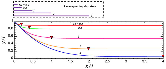
Analytical results for subsurface vapor iso-concentration contour lines for the subslab center concentrations. x/l = 0 is the building center. The downward triangles indicate the characteristic locations of the soil gas samples that should approximate the subslab center vapor concentrations.
Meanwhile, it is of interest to know the location where a soil gas sample taken at some distance from the building would have the same value as css. This vertical position y can be solved for from the linear concentration profile in the uncapped soil:
| (8) |
The value of css needed to obtain y for any values of β/l is available from Eq. (7). The x position can be obtained from Eq. (5), given c = css and the y from Eq. (8). Some characteristic locations of such soil gas samples are indicated by the triangles in Fig. 4.
To illustrate how to apply Eq. (8) and Fig. 4, consider an example in which the building characteristic footprint size is 10 m, and there is no pavement surrounding the building. Assume the contaminant vapor source is 10 m below the slab, then β/l = 1. Assuming ambient vapor concentration to be zero c0 = 0, css using Eq. (7) is predicted to be
| (9) |
Then, the iso-contour line that has the same vapor concentration of 0.455c1 can be found using Eq. (5) which gives the corresponding (x,y) coordinates. This can be done graphically using Fig. 4. In this case, since c0 = 0, from Eq. (8), we have
| (10) |
This allows locating the point corresponding to β/l = 1 and y/l = 0.545 on Fig. 4, which is found at approximately x/l = 1, or 10 m away from the building center, at 5.45 m above the source (or 4.55 m bgs). This is one of the points indicated by the triangles in Fig. 4.
In such a manner, several aspects of a site conceptual model may be verified. For example, if a uniform soil assumption appears to be warranted, and the groundwater source depth has been established, then a comparison of a subslab value with the corresponding Fig. 4 soil gas value can help flag some inappropriate assumption in the site model (e.g. a uniform source or a uniform soil assumption is not warranted). On the other hand, finding agreement between these sample values but then finding a failure to agree with the assumed groundwater source vapor concentration can indicate existence of an intervening resistance (e.g. a capillary fringe) whose value should be accounted for in detailed modeling.
3.2. Approximation to the basement scenario
As far as the authors know, there is no analogous closed-form analytical solution for the iso-concentration contours for a basement scenario, i.e., when the slab exists beneath a basement at some depth below the ground surface. An alternative estimate for this scenario is provided here. The basement depth is taken as lbasement (bgs), as shown in Fig. 5(a), and the soil is assumed homogeneous. The vapor concentration can be easily estimated at a Point B (same depth as the basement slab but away from the influence of the building) as:
| (11) |
Fig. 5.

(a) Basement modeling scenario and (b) Analytical (solid lines) and numerical modeling results (points) for β/l = 0.2, 0.5, 1, and 2.
This is again merely assuming a linear profile in the homogeneous soil. If one now assumes the concentration along a horizontal line AB is a constant (csg_B), i.e., the influence of building on concentration distribution along AB is ignored, we can still apply the previously obtained solution for the slab-on-grade scenario Eqs. (5) and (8), by “moving” the boundary condition from the top of the domain to line AB and redefining c0 in Eqs. (5) and (8) by
| (12) |
It should be emphasized that this does not provide an exact solution, but only an estimate to the solution. This approximate solution using Eqs. (5) and (8) may be compared to the numerical solution, for validation, as is shown in Fig. 5(b). Thus,
| (13) |
For simplicity, now let c0 = 0, so Eq. (11) can be rewritten
| (14) |
We can relate css and c1 by substituting Eq. (14) into Eq. (13):
| (15) |
On the other hand, we can relate css to csg_B by substituting c1 from Eq. (14):
| (16) |
If β/l is fixed at a certain value, the subslab concentration divided by csg_B is a linear function of l/lbasement. This relation is plotted as the solid lines in Fig. 5(b) for different basement sizes and depths. It should be noted that all the lines in Fig. 5(b) would be linear on a linear scale, rather than the log scale used here. When β/l goes to infinity, the first term in Eq. (16) is zero.
The 2D numerical modeling results, simulating the scenario as in Fig. 5(a) are shown as the points in Fig. 5(b). All the points were obtained with the condition that the basement depth is less than half of the building length: lbasement < β/2. The dashed line in Fig. 5(b) is obtained by inserting lbasement = β/2 in Eq. (16). It can be seen that Eq. (16) slightly underestimates the subslab vapor concentration. That is because the concentration along AB is not a constant, but is higher near Point A (as is apparent in Fig. 6, which will be further discussed below).
Fig. 6.

Subsurface contaminant vapor concentration profiles taken from the U.S. EPA report (2012) (EPA, 2012a). Iso-concentration contours that represent the subslab center vapor concentration are shown as the dashed lines. The characteristic locations of soil gas samples that represent the subslab concentration are indicated by the downward triangles, obtained using the present analytical solution. The upward triangles and the other contour lines are from the original EPA report (2012) (EPA, 2012a).
Point B in Fig. 5 represents a shallow soil gas sampling location. Considering the results of a previous study (Shen et al., 2012b), shallow soil gas samples from less than 1 m depth might be influenced by short term meteorological effects, such as a heavy rainfall. The above considerations warn that Eq. (16) and Fig. 5(b) will not be reliable in terms of estimate the subslab vapor concentration using the chosen exterior soil gas concentration at B for shallow B (i.e., < 1 m). In a scenario in which the basement depth is greater than for example 2 m, and the slab to source distance is 2–20 m, then 1 < l/lbasement < 10, Fig. 5(b) shows that the subslab vapor concentration should be within an order of magnitude of the soil gas concentration at B. Here is where such a soil gas measurement should help bound what can be expected subslab, though clearly the estimate will be closer the smaller the ratio of building size to source depth.
For a soil gas probe that is located deeper than the basement slab depth, the iso-concentration contour that has the same concentration as the subslab can be estimated by inserting Eq. (13) into Eq. (5). The method used for the slab-on-grade scenario in Eq. (8) can be used to determine the location of a soil gas probe that should give a soil gas concentration that represents the subslab concentration. The linear concentration gradient away from the building is redefined:
| (17) |
Now, the subslab concentration estimate in Eq. (15) gives the needed relationship between css and β/l. Substitution of Eq. (15) in to Eq. (17) allows calculation of y/l, as before, and Fig. 4 may again be used with this value of y/l and β/l to obtain x/l. That means in the basement scenario, the basement depth does not enter into determining the elevation of the exterior soil gas sampling point that approximates the subslab vapor concentration.
As mentioned in the Introduction, in 2012, the U.S. EPA (2012a) provided simplified examples for comparison between subslab vapor concentration and exterior soil gas vapor concentration using the numerical modeling results, as shown in Fig. 6. The concentration contours are EPA simulation results. The locations of the exterior soil gas samples that could be used to represent subslab vapor concentration are indicated, and shown as the upward triangles for two different source depths. The method provided in this manuscript can now quantitatively estimate the appropriate elevations of the soil gas samples for both slab-on-grade and basement scenarios for any source depths and slab sizes, without resorting to numerical solution. For example, for the basement scenarios shown in Fig. 6, one can use Eq. (15) to predict the subslab vapor concentrations; then use Eq. (20) to calculate the elevations of the exterior soil gas samples. Moreover, one can apply Eqs. (7) and (15) to predict the iso-concentration contours that go through the center of the slab, shown as the dashed lines in Fig. 6.
4. Conclusions
The presented analytical solution provides a simple method to estimate the subsurface contaminant vapor concentration in homogeneous soil vapor intrusion situations. This solution can be used for obtaining estimates for both slab-on-grade and basement scenarios. The analytical results are consistent with the existence of the slab capping effect, which increases the subslab vapor concentration. One of the key factors determining the magnitude of the slab capping effect is the ratio of the slab size or cap size to source depth. It is recommended that more attention be paid in field measurements to collecting information regarding the dimensions of such surface capping features.
Complex transport processes and conditions have been simplified into a relatively simple scenario in the analytical solution. The real world situation can be much more complicated. Analyzing more complicated scenarios, such as those involving heterogeneous soil, non-uniform source, or other factors mentioned in the Introduction, will still require numerical models.
Direct comparison of the present results with the actual field data shown in Fig. 1 is difficult due to lack of building size information in the U.S. EPA database. While it had been previously suggested (Yao et al., 2012c) that other building construction information, such as foundation type and depth be recorded, the recommendation made here concerning collection of building (capping) characteristic size had not yet been formally made. It is the absence of this information that makes the comparison with the EPA dataset problematic.
A U.S. EPA document (2012b) cautioned that “exterior soil gas concentrations collected at depth shallower than 3 m may not be representative of soil gas concentrations measured directly beneath the building foundation”. Further, the U.S. EPA (2012c) has suggested that soil gas samples be taken near the building slab at multiple locations and depths, along with one sample near the source. The relations presented here can help to understand the subsurface vapor concentration distribution, and provide more quantitative guidance as to the locations and depths of such exterior soil gas samples.
HIGHLIGHTS.
A 2D implicit analytical solution is offered describing subsurface vapor concentration.
Building geometrical factors affecting subslab vapor concentration are evaluated.
The analytical solution is compared with numerical modeling results.
Acknowledgments
This project was supported by Grant P42ES013660 from the National Institute of Environmental Health Sciences.
Nomenclature
- c
contaminant vapor concentration (μg m−3)
- c0
open field ambient vapor concentration (μg m−3)
- c1
source vapor concentration in equilibrium with the groundwater (μg m−3)
- csg
soil gas concentration away from the building (μg m−3)
- csg_B
soil gas concentration at Point B (μg m−3)
- css
vapor concentration at the center of the subslab (μg m−3)
- Deff
the effective molecular diffusivity of contaminant in the water and gas phase (m2 s−1)
- Dair
diffusivity of contaminant in the air (m2 s−1)
- g
the acceleration due to gravity (m s−2) acting in the vertical direction z
- keff
the effective soil gas permeability (m2)
- l
the vertical distance from the building slab to source (m)
- l0
source depth below ground surface (m)
- lbasement
basement depth from the open ground (m)
- lsg
vertical distance from soil gas sampling point to source (m)
- lslab
thickness of the building slab (m)
- pg
the soil gas pressure (Pa)
- q
the contaminant mass flux (μg m−2 s−1)
- qcrack
the contaminant mass flux through crack (μg m−2 s−1)
- ug
the superficial velocity of soil gas (m s−1)
- β
characteristic building footprint length (m), including any outdoor pavement
- μg
the soil gas viscosity (kg m−1 s−1)
- ρg
the soil gas density (kg m−3)
- Ω
a function of β/l, defined in Eq. (8) (−)
Appendix A. Schwarz-Christoffel mapping applied to developing Eq. (5)
Schwarz-Christoffel Mapping has been widely used in solving engineering problems, and the mathematical background can be found in various materials (Carslaw and Jaeger, 1959; Krarti et al., 1994; Driscoll and Trefethen, 2002; Yao et al., 2012a). The derivation of Eq. (5) follows from the application of the scenarios shown in Fig. A.1. Fig. A.1(b) illustrates the original domain, with original reference points M, A, B, C and D and the original boundary conditions. This is a difficult problem to solve, since there is a non-simple boundary, represented by the segment MBA. Consider first a simpler scenario represented by Fig. A.1(a), which has only simple boundaries, and how the transform can work on that.
Fig. A.1.

Methodology of the mapping.
A.1. z′-plane to Z-plane
The first step is to obtain the iso-concentration lines in the Z-plane. In Fig. A.1, the Schwarz-Christoffel mapping transforms (a), the z′-plane, into (c) the Z-plane; the angular points A′, B′, C′ and D′ are transformed to A*, B*, C* and D* on the real axis of Z-plane; and boundary conditions are as shown. The transformation relation is:
| (A.1) |
As discussed in Section 2.1, in the z′-plane, the iso-concentration lines are known to be horizontal lines, parallel to the x′ axis:
| (A.2) |
| (A.3) |
Integrating Eq. (A.1), and solve for X and Y, we can obtain the relations:
| (A.4) |
| (A.5) |
Eliminating x′, we have the iso-concentration lines in the Z-plane as:
| (A.6) |
A.2. z-plane to Z-plane
Using the same method above, the transformation relation from (b) z-plane to (c) Z-plane is:
| (A.7) |
where Ω is the x-axis of point M* in the Z-plane, and calculated to be:
| (A.8) |
Again, we can obtain the relations:
| (A.9) |
| (A.10) |
The Schwarz-Christoffel mapping transforms both the z-plane and z′-plane to the same Z-plane. Thus, the iso-concentration lines in the z-plane are:
| (A.11) |
Inserting Eq. (A.3) into Eq. (A.11) and delaminating the solutions out of the geometry domain considered in the z-space, the final iso-concentration line for any known concentration is:
| (A.12) |
Footnotes
Author Disclosure Statement
No competing financial interests exist.
References
- Abreu LDV, Johnson PC. Effect of vapor source-building separation and building construction on soil vapor intrusion as studied with a three-dimensional numerical model. Environ Sci Technol. 2005;39:4550–4561. doi: 10.1021/es049781k. [DOI] [PubMed] [Google Scholar]
- API. Collecting and Interpreting Soil Gas Samples from the Vadose Zone: A Practical Strategy for Assessing the Subsurface Vapor-to-Indoor Air Migration Pathway at Petroleum Hydrocarbon Sites. 2005. [Google Scholar]
- ASTM. Standard Guide for Soil Gas Monitoring in the Vadose zone. American Society for Testing and Materials; West Conshohocken, Pennsylvania: 1992. [Google Scholar]
- Bozkurt O, Pennell KG, Suuberg EM. Simulation of the vapor intrusion process for nonhomogeneous soils using a three dimensional numerical model. Ground Water Monit Rev. 2009;29:92–104. doi: 10.1111/j.1745-6592.2008.01218.x. [DOI] [PMC free article] [PubMed] [Google Scholar]
- Brand E, Otte P, Lijzen J. CSOIL 2000 an Exposure Model for Human Risk Assessment of Soil Contamination. A Model Description. 2007 < http://hdl.handle.net/10029/13385>.
- Carslaw HS, Jaeger JC. Conduction of Heat in Solids. 2. Clarendon Press; Oxford: 1959. p. 1. [Google Scholar]
- Chuangchid P, Krarti M. Steady-periodic three-dimensional foundation heat transfer from refrigerated structures. J Sol Energy Eng. 2000;122:69. [Google Scholar]
- Deru MP, Laboratory NRE. A model for ground-coupled heat and moisture transfer from buildings. Natl Renew Energy Lab 2003 [Google Scholar]
- DeVaull GE. Indoor vapor intrusion with oxygen-limited biodegradation for a subsurface gasoline source. Environ Sci Technol. 2007;41:3241–3248. doi: 10.1021/es060672a. [DOI] [PubMed] [Google Scholar]
- Diallo TMO, Collignan B, Allard F. Build Simul. Springer; pp. xxxxAnalytical quantification of airflows from soil through building substructures; pp. 1–14. [Google Scholar]
- Driscoll TA, Trefethen LN. Schwarz-Christoffel Mapping. Cambridge University Press; 2002. [Google Scholar]
- Eklund B, Beckley L, Yates V, McHugh TE. Overview of state approaches to vapor intrusion. Remediat J. 2012;22:7–20. [Google Scholar]
- EPA. Conceptual Model Scenarios for the Vapor Intrusion Pathway. U.S. Environmental Protection Agency; Washington, DC: 2012a. [Google Scholar]
- EPA. EPA’s Vapor Intrusion Database: Evaluation and Characterization of Attenuation Factors for Chlorinated Volatile Organic Compounds and Residential Buildings. 2012b. 530-R-10-002, E. (Ed.) [Google Scholar]
- EPA. Superfund vapor intrusion FAQs. 2012c In: < http://www.epa.gov/oswer/vaporintrusion/guidance.html#Item5> (Ed.)
- Ferguson C, Krylov V, McGrath P. Contamination of indoor air by toxic soil vapours: a screening risk assessment model. Build Environ. 1995;30:375–383. [Google Scholar]
- Hers I, Zapf Gilje R, Johnson PC, Li L. Evaluation of the Johnson and Ettinger model for prediction of indoor air quality. Ground Water Monit Rev. 2003;23:119–133. [Google Scholar]
- Johnson PC. Identification of critical parameters for the Johnson and Ettinger (1991) vapor intrusion model. Am Pet Inst. 2002;17:1–N2. [Google Scholar]
- Johnson PC, Ettinger RA. Heuristic model for predicting the intrusion rate of contaminant vapors into buildings. Environ Sci Technol. 1991;25:1445–1452. doi: 10.1021/acs.est.8b01106. [DOI] [PubMed] [Google Scholar]
- Karapanagioti HK, Gaganis P, Burganos VN. Modeling attenuation of volatile organic mixtures in the unsaturated zone: codes and usage. Environ Modell Softw. 2003;18:329–337. [Google Scholar]
- Krarti M, Claridge DE, Kreider JF. The ITPE technique applied to steady-state ground-coupling problems. Int J Heat Mass Transfer. 1988;31:1885–1898. [Google Scholar]
- Krarti M, Kreider JF, Claridge DE. Schwarz-Christoffel transformation applied to steady-state ground-coupling problems. Energy Build. 1994;20:193–203. [Google Scholar]
- Little JC, Daisey JM, Nazaroff WW. Transport of subsurface contaminants into buildings. Environ Sci Technol. 1992;26:2058–2066. [Google Scholar]
- Luo H, Dahlen P, Johnson PC, Peargin T, Creamer T. Spatial variability of soil-gas concentrations near and beneath a building overlying shallow petroleum hydrocarbon-impacted soils. Ground Water Monit Rev. 2009;29:81–91. [Google Scholar]
- McAlary TA, Nicholson P, Groenevelt H, Bertrand D. A case study of soilgas sampling in silt and clay-rich (low-permeability) soils. Ground Water Monit Rev. 2009;29:144–152. [Google Scholar]
- McHugh TE, Beckley L, Bailey D, Gorder K, Dettenmaier E, Rivera-Duarte I, Brock S, MacGregor IC. Evaluation of vapor intrusion using controlled building pressure. Environ Sci Technol. 2012;46:4792–4799. doi: 10.1021/es204483g. [DOI] [PubMed] [Google Scholar]
- Mills WB, Liu S, Rigby MC, Brenner D. Time-variable simulation of soil vapor intrusion into a building with a combined crawl space and basement. Environ Sci Technol. 2007;41:4993–5001. doi: 10.1021/es061747d. [DOI] [PubMed] [Google Scholar]
- Nazaroff W. Predicting the rate of 222Rn entry from soil into the basement of a dwelling due to pressure-driven air flow. Radiat Prot Dosim. 1988;24:199. [Google Scholar]
- Olson DA, Corsi RL. Characterizing exposure to chemicals from soil vapor intrusion using a two-compartment model. Atmos Environ. 2001;35:4201–4209. [Google Scholar]
- Pacific S. Rev Best Practices. 2009. Review of best practices, knowledge and data gaps, and research opportunities for the US Department of Navy Vapor Intrusion Focus Areas. [Google Scholar]
- Pennell KG, Bozkurt O, Suuberg EM. Development and application of a three-dimensional finite element vapor intrusion model. J Air Waste Manage. 2009;59:447–460. doi: 10.3155/1047-3289.59.4.447. [DOI] [PMC free article] [PubMed] [Google Scholar]
- Picone S, Valstar J, van Gaans P, Grotenhuis T, Rijnaarts H. Sensitivity analysis on parameters and processes affecting vapor intrusion risk. Environ Toxicol Chem. 2012;31:1042–1052. doi: 10.1002/etc.1798. [DOI] [PubMed] [Google Scholar]
- Provoost J, Reijnders L, Swartjes F, Bronders J, Seuntjens P, Lijzen J. Accuracy of seven vapour intrusion algorithms for VOC in groundwater. J Soil Sediment. 2009;9:62–73. [Google Scholar]
- Robinson AL, Sextro RG, Fisk WJ. Soil-gas entry into an experimental basement driven by atmospheric pressure fluctuations—measurements, spectral analysis, and model comparison. Atmos Environ. 1997;31:1477–1485. [Google Scholar]
- Sanders PF, Hers I. Vapor intrusion in homes over gasoline contaminated ground water in Stafford, New Jersey. Ground Water Monit Rev. 2006;26:63–72. [Google Scholar]
- Shen R, Pennell KG, Suuberg EM. A numerical investigation of vapor intrusion—the dynamic response of contaminant vapors to rainfall events. Sci Total Environ. 2012b;437:110–120. doi: 10.1016/j.scitotenv.2012.07.054. [DOI] [PMC free article] [PubMed] [Google Scholar]
- Shen R, Pennell KG, Suuberg EM. Evaluation of the influence of soil moisture on soil gas vapor concentration in vapor intrusion. Environ Sci Eng. 2013a doi: 10.1089/ees.2013.0133. (in press) [DOI] [PMC free article] [PubMed] [Google Scholar]
- Shen R, Yao Y, Pennell KG, Suuberg EM. Modeling quantification of the influence of soil moisture on subslab vapor concentration. Environ Sci: Processes Impacts. 2013b;15 (7):1444–1451. doi: 10.1039/c3em00225j. [DOI] [PMC free article] [PubMed] [Google Scholar]
- Suuberg E, Yao Y, Shen R, Bozkurt O, Pennell K. Modeling vapor intrusion processes and evaluating risks using subslab data. Environ Health Biomed. 2011;15:115. [Google Scholar]
- Tillman FD, Weaver JW. Temporal moisture content variability beneath and external to a building and the potential effects on vapor intrusion risk assessment. Sci Total Environ. 2007;379:1–15. doi: 10.1016/j.scitotenv.2007.02.003. [DOI] [PubMed] [Google Scholar]
- Turczynowicz L, Robinson NI. Exposure assessment modeling for volatiles— towards an Australian indoor vapor intrusion model. J Toxicol Environ Health. 2007;70:1619–1634. doi: 10.1080/15287390701434711. [DOI] [PubMed] [Google Scholar]
- Van Sant J. The spot-insulated plate. Nucl Eng Des. 1968;8:247–250. [Google Scholar]
- Yao Y, Shen R, Pennell KG, Suuberg EM. Comparison of the Johnson–Ettinger vapor intrusion screening model predictions with full three-dimensional model results. Environ Sci Technol. 2011;45:2227–2235. doi: 10.1021/es102602s. [DOI] [PMC free article] [PubMed] [Google Scholar]
- Yao Y, Pennell KG, Suuberg EM. Estimation of subslab concentration in vapor intrusion. J Hazard Mater. 2012a;231–232:10–17. doi: 10.1016/j.jhazmat.2012.06.016. [DOI] [PMC free article] [PubMed] [Google Scholar]
- Yao Y, Pennell KG, Suuberg EM. Simulating the effect of slab features on vapor intrusion of crack entry. Build Environ. 2012b;59:417–425. doi: 10.1016/j.buildenv.2012.09.007. [DOI] [PMC free article] [PubMed] [Google Scholar]
- Yao Y, Shen R, Pennell KG, Suuberg EM. Examination of the influence of environmental factors in contaminant vapor concentration attenuation factor with U.S. EPA’s vapor intrusion database. Environ Sci Technol. 2012c;47:906–913. doi: 10.1021/es303441x. [DOI] [PMC free article] [PubMed] [Google Scholar]
- Yao Y, Shen R, Pennell KG, Suuberg EM. Estimation of contaminant subslab concentration in vapor intrusion including lateral source-building separation. Vadose Zone J. 2013a doi: 10.2136/vzj2012.0157. http://dx.doi.org/10.2136/vzj2012.0157. [DOI] [PMC free article] [PubMed]
- Yao Y, Shen R, Pennell KG, Suuberg EM. Examination of the U.S. EPA’s vapor intrusion database based on models. Environ Sci Technol. 2013b;47 (3):1425–1433. doi: 10.1021/es304546f. [DOI] [PMC free article] [PubMed] [Google Scholar]
- Yao Y, Shen R, Pennell KG, Suuberg EM. A review of vapor intrusion models. Environ Sci Technol. 2013c;47 (6):2457–2470. doi: 10.1021/es302714g. [DOI] [PMC free article] [PubMed] [Google Scholar]
- Yu S, Unger AJA, Parker B. Simulating the fate and transport of TCE from groundwater to indoor air. J Contam Hydrol. 2009;107:140–161. doi: 10.1016/j.jconhyd.2009.04.009. [DOI] [PubMed] [Google Scholar]