Accelerated multi-shot diffusion imaging

Abstract

Purpose:

To reduce image distortion in MR diffusion imaging using an accelerated multi-shot method.

Methods:

The proposed method exploits the fact that diffusion-encoded data tend to be sparse when represented in the k_b-k_d space, where k_b and k_d are the Fourier transform duals of b and d, the b-factor and the diffusion direction, respectively. Aliasing artifacts are displaced toward under-utilized regions of the k_b-k_d plane, allowing non-aliased signals to be recovered. A main characteristic of the proposed approach is how thoroughly the navigator information gets utilized during reconstruction: The phase of navigator images is used for motion correction, while the magnitude of the navigator signal in k_b-k_d space is used for regularization purposes. As opposed to most acceleration methods based on compressed sensing, the proposed method reduces the number of k_y lines needed for each diffusion-encoded image, but not the total number of images required. Consequently, it tends to be most effective at reducing image distortion rather than reducing total scan time.

Results:

Results are presented for three volunteers with acceleration factors ranging from 4 to 8, with and without the inclusion of parallel imaging.

Conclusion:

An accelerated motion-corrected diffusion imaging method was introduced that achieves good image quality at relatively high acceleration factors.

Introduction

Over the last two decades, MR diffusion-weighted imaging (DWI) has evolved into an immensely useful tool to assess stroke, tissue fiber architecture, and characteristic tissue water diffusion. However, motion sensitivity remains a serious problem in DWI. Diffusion-encoding gradients are designed for detecting the small displacements of water molecules, and as a consequence, sensitivity to other types of (undesired) motion such as bulk or physiological motion appears unavoidable. Even fairly subtle motion, in conjunction with diffusion-encoding gradients, may cause substantial phase variations throughout the imaged object. To protect against artifacts that might arise from such phase instability, single-shot 2D echo-planar imaging (EPI) is typically employed in DWI to generate ‘snapshot’ images of the object, so that the error-prone phase information might be safely dismissed from every snapshot image. While the single-shot EPI sequence offers an effective means of avoiding for the most part motion-induced phase problems, it comes at the cost of severe limitations in overall image quality, especially in terms of geometric fidelity.

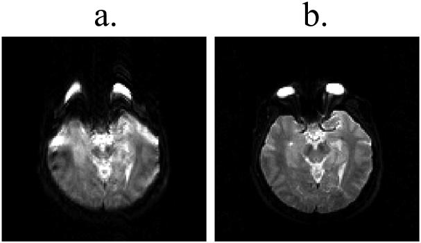
Rather than discarding the phase information, one might instead use navigator echoes to detect and account for unexpected phase variations (1-7). One of the main benefits of preserving the phase information is to enable multi-shot DWI, whereby k-space is sampled over several TR periods rather than a single one. Multi-shot imaging can be used, for example, to alleviate the geometrical distortion problems that tend to plague single-shot imaging (e.g., see Fig. 1). Multi-shot imaging may even enable 3D DWI, where 3D images may be acquired with improved SNR and through-slice resolution compared to present 2D implementations (8, 9). However, multi-shot imaging can readily lead to prohibitively-long scan times, and the method proposed here was designed to accelerate the acquisition of multi-shot DWI datasets. As compared to a single-shot EPI sequence as typically used in DWI, the proposed approach enables improvements in image quality, especially in terms of geometric distortion, at potentially no cost in scan time.

Fig. 1.

Single-shot EPI images may greatly suffer from geometric distortions, as shown in (a), a problem that can be very much alleviated using k-space segmentation, as shown in (b). The acquisition in (b) was made over 4 TR intervals as opposed to a single TR interval in (a), and these 4-shot data were reconstructed as described in Ref. (1). The main goal of the present work was to accelerate multi-shot imaging, to make it essentially as fast as single-shot imaging while preserving the geometric-fidelity advantages seen here. (The single-shot image in (a) was acquired using 80 echoes, 62.5% partial-Fourier, echo spacing = 668 μs, matrix size = 128×128, FOV = 25.6 cm, TR = 3 s, 4 mm slice, b ≈ 0 s/mm². The four-shot image in (b) involved the same parameters as above, except for 32 echoes per echo train, no partial-Fourier and echo spacing = 664 μs).

The present method is based on the observation that DWI data tend to be very sparse when represented in a k_b-k_d space, where k_b and k_d are the conjugate variables associated with b and d, the b-factor and diffusion direction, respectively. While b is measured as usual in s/mm², d is simply a dimensionless integer counting the different diffusion-encoding directions being sampled. The accelerated multi-shot DWI technique presented here was designed to fully utilize the available navigator information, for both motion compensation and regularization purposes. While reliable navigator-based motion-compensation strategies already exist for DWI (e.g., Atkinson et al. (1)), such methods employ only the phase of navigator images and discard the magnitude information. In contrast, acceleration methods such as k-t BLAST (10) use the magnitude information of training images in x-y-f space for regularization purposes and discard the phase information. The present method proposes an integrated way of fully exploiting the information from navigator scans, to perform accelerated and motion-compensated multi-shot DWI. While the phase of the navigator-images is used in a way consistent with Atkinson et al. (1) to compensate for motion-induced phase variations, the magnitude of the navigator-images in x-y-k_b-k_d space is used to provide both a regularization term and an initial guess toward the numerical solution of the under-sampled imaging problem. In terms of k-space sampling strategy, the present method involves shifting the sampling function along the k_y and/or k_z direction(s) from one b value to the next and from one d value to the next. In other words, only a subset of all interleaved EPI segments are acquired for each diffusion-weighted image and the choice of which segments are sampled and which ones are skipped is modified according to b and d.

As demonstrated in the Results section, the proposed approach allows sizeable acceleration rates to be achieved, in a manner that proves readily compatible with additional acceleration methods such as parallel imaging, or partial-Fourier imaging. The proposed approach may also possibly prove compatible with compressed sensing as applied to DWI (11), although a proper demonstration should be considered beyond the scope of the present work. While our approach aims to subsample the k_y axis and thus improve image quality, compressed sensing typically aims to reduce the total number of diffusion-encoded images required and thus reduce scan time. As our approach and compressed sensing tend to act differently, on different dimensions, and for slightly different purposes, it seems reasonable to believe they might be applied jointly. More generally, modern acceleration schemes often combine a number of different individual strategies for added effect, and the present approach may well prove a worthwhile contributor to the mix.

Some of the results presented here were acquired using a single-channel quadrature head coil, to emphasize the fact that acceleration is obtained in a manner entirely distinct from parallel imaging. Results from a phased-array head coil where the proposed approach is combined with parallel imaging are also presented, to show that both methods can readily be combined for added effect. Acceleration up to 6-fold was reached when using the proposed method by itself (using a quadrature head coil), and acceleration up to 8-fold was obtained when further including parallel imaging (using an 8-channel head coil).

Theory

1. Least-square solution and phase correction

As usual in accelerated imaging, the reconstruction problem can be expressed as a matrix multiplication:

$$\mathit{s}=\mathbf{E}\times \mathit{o},$$ [1]

where s is a vector containing the acquired signal, o is a vector containing the object-related data to be reconstructed, and E is the encoding matrix relating the two. The least-square solution to the problem from Eq. [1] can be expressed as (12):

$$\widehat{o}={({\mathbf{E}}^{\mathrm{H}}\times {\Psi }^{-1}\times \mathbf{E}+{\lambda }^2\mathbf{L})}^{-1}\times {\mathbf{E}}^{\mathrm{H}}\times {\Psi }^{-1}\times \mathit{s},$$ [2]

where ô is an estimated version of o, E^H×Ψ^-1 is a preconditioning term, λ²L is a damped least-squares regularization term, and the superscript ‘H’ represents a Hermitian transpose operation. In the present implementation, Ψ was simply equated to an identity matrix.

Much of the present work is based on the observation that the data in o tend to be very sparse when represented in the x-y-k_b-k_d space, where k_b and k_d are the Fourier transform duals of b and d, the b-factor and diffusion direction, respectively. For this reason, it seems natural to represent both ô and s from Eq. 2 in this x-y-k_b-k_d space. The present method has much in common with the phase-corrected multi-coil navigated method from Atkinson et al. (1), and the expression for the encoding matrix, as presented below in Eq. 3, is similar in form to Eq. 1 from Ref. (1):

$${\mathbf{E}}_j=\sum _i({\mathbf{F}}_d\times {\mathbf{F}}_b\times {\mathbf{F}}_y^H\times {\mathbf{W}}_i\times {\mathbf{D}}_i\times {\mathbf{F}}_y\times {\mathbf{c}}_j\times {\mathbf{p}}_i\times {\mathbf{F}}_d^H\times {\mathbf{F}}_b^H),$$ [3]

where F_y, F_b and F_d perform Fourier transforms along y, b and d, respectively, p_i is a motion-related phase correction (from navigator data), D_i subsamples k-space, c_j is the sensitivity map for coil j, W_i can be used to suppress unreliable data, and the summation is made over all interleaved segments, from i = 1 to i = N_s, the number of shots per frame. N_s is given by the total number of interleaves that would be needed to fully sample the k-space matrix, N_I, divided by the acceleration factor, R, so that N_s = N_I / R. E_j in Eq. 3 is specific to a single coil element, j, and the full E matrix as expressed in Eqs 1 and 2 is obtained by pasting vertically all E_j sub-matrices:

$$\mathbf{E}=\left[\begin{array}{c}\hfill {\mathbf{E}}_1\hfill \\ \hfill ⋮\hfill \\ \hfill {\mathbf{E}}_{NC}\hfill \end{array}\right],$$ [4]

where N_c is the total number of coil elements. Assuming that full k_x lines are acquired, as is typically the case with an EPI sequence, the processing in Eqs 2-4 (as well as that from Atkinson et al. (1)) can be performed one x location at a time, for faster processing. Furthermore, assuming regular down-sampling along k_y, only R pixels in the y direction need to be considered at a time. In other words, when sampling full k_x lines with regular down-sampling along k_y, the processing in Eqs 2-4 can be repeated (N_x×N_y /R) times using E matrices consisting of only R×N_b×N_d×N_c columns, as opposed to the most general case where processing would be performed only once using a much larger E matrix consisting of N_x×N_y×N_b×N_d×N_c columns.

At first sight, the main difference between Ej from Eq. 3 and the bracketed expression in Eq. 1 of Ref. (1) is the presence of Fourier transforms along the b and d axes, i.e., the F_d×F_b and the F_d^H×F_b^H terms. A possibly more meaningful difference comes from the fact that E_j in Eq. 3 operates on a 3-D space (e.g., y-k_b-k_d, or k_y-b-d) rather than a 1-D space (y or k_y). As explained below, further differences emerge in the choice of the sampling scheme, D_i, and of a regularization term, λ²L.

2. Selecting the sampling scheme D_i (from Eq. 3)

D_i in Eq. 3 is a diagonal matrix of size R×N_b×N_d×N_c, (assuming that full k_x lines are sampled using regular down-sampling along k_y, as discussed above). The elements of D_i are all equal to either zero or one, and all non-zero entries are found along the main diagonal. The problem of selecting a D_i matrix boils down to deciding which one(s) of the N_I interleaves should be sampled, for each combination of diffusion-encoding parameters, b and d. Given R different and complementary ways of sampling a fraction 1/R of the k-space matrix, the elements in D_i determine which one of these R different ways gets employed for each one of the N_b×N_d diffusion-weighted images being acquired. The most desirable D_i matrix would be one that minimizes the condition number of the associated E matrix (Eq. 3), for a given acceleration factor, R.

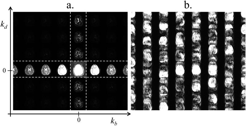
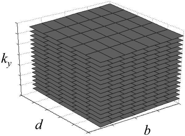
Discriminating desirable signals from artifactual signals is typically easiest when the amount of overlap between these two types of signals is minimal to begin with. Figure 2a shows N_d×N_b in vivo diffusion-weighted images tiled side-by-side along k_b and k_d axes, with each image N_x by N_y pixels in size. A striking feature of the display in Fig. 2a is that most of the signal can be found at locations where k_b and/or k_d = 0, i.e., within the cross-shaped region highlighted with white dashed lines in Fig. 2a. Using an acceleration factor R, R-1 replicas of the signals from Fig. 2a may get created. One particular sampling scheme, described in more details below, has the ability to displace these R-1 replicas and spread them all across the k_b-k_d plane. This is shown in Fig. 2b, although it should be kept in mind that signals in Fig. 2b are further complicated by phase inconsistencies as described by the term p_i in Eq. 3. Because much of the signal from Fig. 2b falls in regions of the k_b-k_d plane left mostly unused by desirable signal such as in Fig. 2a, the amount of overlap between desirable and artifactual signals is relatively low to begin with, which tends to facilitate the solving of the linear problem as modeled through Eqs 1-4. The displacement of the R-1 replica as shown in Fig. 1b was achieved by shifting the sampling function by one Δk_y increment from one b value to the next as well as from one d value to the next, in a 2D equivalent of the sampling scheme used in the ‘unaliasing by Fourier-encoding the overlaps in the temporal direction’ (UNFOLD) method (13). A 3D plot of the sampled k_y locations as a function of both b and d is shown in Fig. 3. The matrix D_i in Eq. 3 is a diagonal matrix, and the entries along its diagonal could be obtained from the plot in Fig. 3 as follows: All locations along the planes in Fig. 3 would be given a value of one, all other locations a value of zero, only the first R locations along k_y are kept, the resulting R×N_b×N_d 3-D grid is reformatted into a 1D column-vector, and this column vector is replicated N_c times to get the R×N_b×N_d×N_c diagonal entries.

Fig. 2.

a) Diffusion-weighted images for 7 different b-values, from 202 to 1414 s/mm², and 6 different directions were Fourier transformed along the b and d directions (the imaging parameters are the same as in Fig. 1a). Most signal is concentrated in the cross-shaped region characterized by k_b = 0 and/or k_d = 0, highlighted with white dashed lines. b) Subsampling k_y by a factor 4 leads to a more complicated k_b × k_d space, heavily corrupted by aliasing artifacts. The fact that the desired solution tends to be sparse, as seen in (a), greatly facilitates the task of numerically sorting out the signal in (b). In addition to aliasing artifacts caused by 4-fold subsampling, the signal in (b) is further complicated by motion-induced and possibly drift-induced phase variations in b-d space, i.e., the term p_i from Eq. 3.

Fig. 3.

The subsampling scheme can be visualized in a k_y-b-d space. In the present example, 16 planes separated by 8 k_y lines would be acquired to reconstruct 128 y locations with an acceleration factor of 8. Intersecting black lines indicate the sampled b-d locations. A cross-section of these planes in a k_y-b plane would give straight lines with slope ∆k_y/∆b, where ∆k_y is the distance between consecutive k_y lines and ∆b is the distance between consecutive b values, while a cross-section in a k_y-d plane would give straight lines with slope ∆k_y.

3. Adjusting the regularization term λ²L (from Eq. 2)

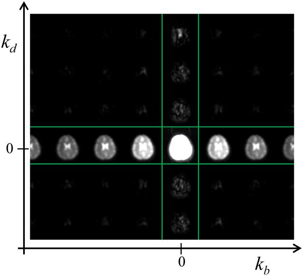
Figure 4 shows a navigator dataset in the same format also used in Fig. 2a. The main difference between the data from Fig. 2a and navigator data from Fig. 4 comes from the fact that navigator acquisitions cover only a small central region in k-space, and thus the navigator data in Fig. 4 are spatially blurred. Zero-padding in k-space was used to interpolate navigator images to N_x×N_y pixels, the same matrix size as for the imaging data. In a way similar to the work in (10), a diagonal matrix M is defined here whose diagonal consists of magnitude values from a training scan. In the present case, there is no training scan per se, but data from the navigator scan can be used instead. The main diagonal of M consists of R×N_b×N_d×N_c magnitude values taken from the navigator data, and correspond to the x-y-k_b-k_d locations for which a solution is being sought, i.e., to all b and d values for a given location along x and a given set of R locations along y. For reasons discussed in (14), the M matrix is normalized here by its Froebinius norm, ||M||₂, to make the regularization term insensitive to arbitrary scaling factors and gains that might affect the acquired data. The regularization-related matrix L is thus given by:

$$\mathbf{L}={\left(\frac{\mathbf{M}}{\mid \mid \mathbf{M}\mid {\mid }_2}\right)}^{-2},$$ [5]

and the regularization term λ²L in Eq. 2 is obtained by multiplying L in Eq. 5 by λ².

Fig. 4.

The magnitude of the navigator images, in x-y-d-b space, is Fourier transformed to x-y-k_d-k_b space. The magnitude of the result, displayed here, is used toward generating the regularization term L in Eq. 2, as described in the text.

4. On further generalizing Eq. 3

Most of the results presented here were obtained using a Cartesian sampling scheme in b-d space, in other words, all N_d encoding directions are sampled for each one of the selected N_b b-factors. Results for a high angular resolution diffusion sampling scheme (15), whereby a single non-zero b-value is sampled (N_b = 2, b_max = 2000 s/mm² and N_d = 100), are also presented. Many other useful sampling schemes have been proposed, such as Hybrid Diffusion Imaging (HYDI) (15) or Diffusion Spectrum Imaging (DSI) (16). The present work focuses for the most part on a Cartesian sampling scheme in b-d space because, for this special case, we have identified a simple D_i sampling scheme in k_y-b-d space capable of very much limiting the amount of overlap between desirable and artifactual signals, as shown in Figs 2 and 3. While generalizing Eq. 3 to other types of diffusion encoding schemes might be mostly trivial, identifying appropriate D_i matrices for these non-Cartesian diffusion encoding schemes is less obvious.

Methods

1. MR setup and pulse sequence

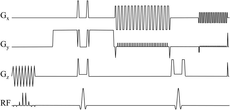
Imaging was performed on a 3.0 T MR system (GE Signa CVi, Milwaukee, WI, 40 mT/m, 150 T/m/s). Our navigated multi-shot EPI sequence included a spectral-spatial RF excitation, a pair of diffusion-encoding gradient pulses, two refocusing pulses, a first EPI echo train to gather imaging data and a second echo train to gather navigator data (see Fig. 5). In the present implementation, the acquisition was not ECG-gated and b-values were linearly distributed between zero and a maximum setting, b_max; although not implemented here, the proposed work should prove readily compatible with ECG-gating and/or non-uniform sampling of the b axis.

Fig. 5.

Our navigated multi-shot EPI sequence is depicted here. See text for more details.

The following MR imaging parameters were common to all scans: Axial slices, frequency encoding along R/L, thickness = 4 mm, spacing between slices = 4 mm, TR = 3000 ms, echo-train length for imaging data = 32, echo-train length for navigator data = 32 and ramp-sampled readouts. A bandwidth of ±250 kHz was employed in all cases except for the R = 8 scans, which involved a narrow 17.0 cm FOV along the frequency-encoding direction, for which a bandwidth of ±167 kHz was employed instead. Other imaging parameters varied from scan to scan, and parameters for the human scans are listed in Table 1. Some datasets were acquired using a single-channel quadrature head coil, to help demonstrate that the proposed approach can accelerate scans independently of parallel imaging, while others were acquired using an 8-channel head coil instead, for improved results.

Table 1.

imaging parameters

#	Subject	Coil(a)	R	Matrix	Nb (b)	bmax s/mm2	Nd	TE/TEnav ms	ESP/ESPnav(c) μs	BWy/BWynav(d) kHz	Nz (e)	FOV cm2
1	1	8	6	192×192	8	1414	6	71.8/106.2	800/320	7.50/3.1	10	22.0×22.0
2	1	8	8	192×256	8	1414	6	76.9/116.4	952/364	8.40/2.75	10	17.0×22.7
3	1	Q	4	128×128	8	1414	6	66.3/95.3	640/320	6.25/3.13	10	22.0×22.0
4	1	Q	6	192×192	8	1414	6	71.8/106.2	800/320	7.50/3.13	10	22.0×22.0
5	2	8	4	128×128	2	2000	100	83.9/113.3	652/328	6.13/3.05	9	22.0×22.0
6	2	8	6	192×192	8	1414	6	71.8/106.2	800/320	7.50/3.13	9	22.0×22.0
7	2	8	8	192×256	8	1414	6	76.9/116.4	952/364	8.40/2.75	10	17.0×22.7
9	3	8	4	128×128	8	2500	6	75.0/104.1	640/320	6.25/3.13	10	22.0×22.0
10	3	8	8	192×256	4	708	6	68.4/108.0	952/352	8.40/2.84	9	17.0×22.7
11	3	Q	6	192×192	4	708	6	63.3/97.7	800/312	7.50/3.21	9	22.0×22.0

^(a)Either ‘Q’ for quadrature head coil, or ‘8’ for 8-channel head coil

^(b)N_b, the number of sampled b-factors, including the b ≈ 0 case

^(c)ESP is the echo-spacing for the imaging data, and ESP_nav for the navigator data

^(d)Acquisition bandwidth along y, where BWy = (R/ESP) and BWy_nav = (1/ESP_nav)

^(e)N_z is the number of slices

Scan time for all b > 0 data was equal to (N_b – 1) × N_d × TR, while scan time for the T2-weighted image was equal to R × TR. Phase-encoding was turned off for the first 3 TR intervals, to provide reference data toward EPI-ghost correction. The total scan time was thus ((N_b – 1)×N_d + R + 3) × TR. In Fig. 5, the sequence as displayed was obtained using the following set of imaging parameters: Matrix size = 128x128, echo-train length = 32 echoes, 4-fold acceleration, b = 150 s/mm²", FOV = 22 cm, slice thickness = 4 mm, TE = 51 ms, TE_nav = 81 ms.

2. Image reconstruction

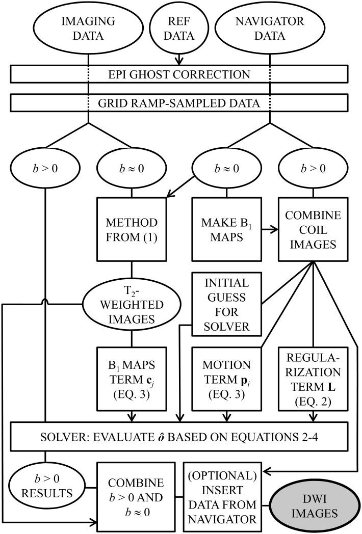
Image reconstruction was performed in Matlab (The MathWorks, Natick, MA), using a DELL Precision T7500 (Round Rock, Texas, USA). Figure 6 gives a schematic representation of the reconstruction algorithm. Because it has no directional dependence, the b ≈ 0 data could be fully sampled at little cost in scan time, and this is why these data are treated differently from the b > 0 data in Fig. 6. The fully-sampled b ≈ 0 data were reconstructed, with motion correction, using the method from Ref. (1); the resulting T₂-weighted images were then employed toward calculating the B₁ sensitivity maps, i.e., the c_j term in Eq. 3. Similarly, the b ≈ 0 navigator data were also used to generate B₁ sensitivity maps, to combine the navigator images from different coil elements. The navigator signal was first filtered along the k_x and k_y directions using a Fermi apodization filter, to suppress ringing artifacts, and all coil images were then combined using the navigator-derived B₁ sensitivity maps. Because different B₁ sensitivity maps were used for the imaging data than for the navigator data, phase inconsistencies between these two signal types could be ‘absorbed’ into the B₁ maps, making them compatible for eventual merger (as further described below).

Fig. 6.

The reconstruction algorithm takes as an input the acquired imaging data, the navigator data, and the reference data (i.e., three TR worth of data acquired without any phase encoding). Aliasing-free diffusion-weighted images are generated at the output. These images can then be analyzed, as usual, to calculate the diffusion tensor for each image voxel. A key characteristic of the method is how thoroughly the navigator data get utilized: To obtain a motion-correction phase term, a regularization magnitude term, an initial guess for the iterative solver and, optionally, for direct replacement of the central k-space region in the final results. See text for more details.

A main characteristic of the proposed approach is how thoroughly the navigator information gets exploited, as can be appreciated by the number of branches that follow the ‘combine coil images’ operation in Fig. 6, in the ‘navigator data’ part of the flowchart. The coil-combined navigator data were used for motion correction (term p_i in Eq. 3), for regularization (term L in Eq. 3), to initialize the iterative solver, and optionally to substitute the low spatial frequency information in the final DWI results. All acquired imaging data were motion-corrected, i.e., none were outright rejected, meaning that the term W_i in Eq. 3 was equated to an identity matrix. While rejecting some of the most heavily-corrupted data might well prove advantageous, such feature was not part of our present implementation. As mentioned above, using different B₁ maps for imaging and navigator data allowed phase inconsistencies to be handled, and a scaling factor was obtained by comparing all k-space locations that were sampled in both the imaging and navigator datasets, making the two compatible for merger. Different T₂ weightings and potentially slightly-different geometrical distortions could be sources of artifacts when performing such merger, which was treated as an option in the implementation. In our experience, this option proved particularly helpful for results obtained at higher acceleration settings and did not appear to negatively impact image quality even at lower acceleration settings, and for these reasons it was employed in all of the results presented here.

The diffusion-weighted images generated as an output in Fig. 6 could be analyzed, in a usual manner, to calculate the diffusion tensor, apparent diffusion coefficient (ADC), fractional anisotropy (FA), kurtosis parameters (17) or even fiber crossings at every image voxel. All available b-factors were used in all fits.

3. Phantom imaging

SNR tests were performed in a diffusion phantom consisting of celery in a water bath using minimal diffusion weighting (b_max = 20 s/mm², R = 4, single-channel quadrature head coil, 128x128 matrix, TE/TE_nav = 34.3/60.6 ms, echo spacing (ESP) / ESP_nav = 604/304 μs, FOV 9 = 25.6x25.6 cm²). A total of 144 images (N_d = 6, N_b, = 24) were reconstructed, and as a consequence of the very low b_max setting, these images were mostly equivalent to each other except for noise. The magnitude signal in the raw (aliased) images and in the reconstructed (de-aliased) images had identical scaling.

Noise in the raw images was measured as the standard deviation in the real channel across all 144 raw images. A noise value n_a was obtained for the aliased images by averaging the standard deviation map over a small 3×3 ROI located in the void, outside of the imaged phantom. Noise in the reconstructed images was similarly measured as the standard deviation in the real channel across all 144 reconstructed images. But unlike what was done for n_a above, the noise value for reconstructed images n_r was obtained from a 3×3 ROI located within the phantom, not in the void around it.

4. Human imaging

Three human volunteers were imaged with the proposed method following informed consent with an IRB-approved protocol. For comparison purposes, DWI results were reconstructed using parallel-imaging as the only source of acceleration when possible, i.e., when a multi-channel coil was employed. To do so, our reconstruction algorithm was converted into a more basic (but still motion-corrected) reconstruction by replacing L in Eq. 2 with an identity matrix to obtain a zeroth-order Tikhonov regularization scheme (λ² = 0.02), and by turning off the k-space center substitution scheme described above.

Results

1. Reconstruction example

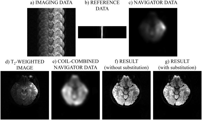
As exemplified in Fig. 1, the main advantage provided by the proposed method over regular single-shot non-accelerated DWI is a marked improvement in geometric fidelity, especially for locations near the sinuses. Figure 7 details the reconstruction process for one given slice from one given scan, to help better understand how the algorithm from Fig. 6 functions. The input to the algorithm, the imaging, reference and navigator data, can be visualized in Figs 7a-c. Some of the intermediate results, the T₂-weighted image and the navigator image, can be visualized in Figs 7d and 7e, while the reconstructed results with and without the optional data substitution are shown in Figs 7f and 7g. Images that correspond to a single b-value and diffusion-encoding direction were selected for display purposes: b = 471 s/mm and the second diffusion-encoding orientation (out of six). It may be noted that the aliasing artifacts, clearly visible in the input imaging data (Fig. 7a), were very effectively suppressed in the reconstructed results (Figs 7f and 7g).

Fig. 7.

The images shown here aim to illustrate key steps of the algorithm from Fig. 6. a-c) The input to the algorithm from Fig. 6 consists of imaging data, navigator data and at least one TR worth of non-phase-encoded reference data to correct for EPI ghosting artifacts. d) The fully-sampled b ≈ 0 data were reconstructed using the method from (1), one coil-element at a time (coil element 2/8 here). e) All coil elements were combined for the navigator data, and the resulting images were used for motion-correction, regularization, solver initialization and optionally for direct data replacement (see Fig. 6). f,g) The reconstructed result is displayed with and without the optional data replacement, which had little effect in this particular case. The dataset was acquired using R = 6, 192×192 matrix size, N_b = 4, N_d = 6, and the 9 displayed slice corresponds to b = 471 s/mm².

2. SNR tests in phantom

The ratio between noise in the aliased images, n_a, and in the reconstructed images, n_r, was measured as described in the Methods section, for an R = 4 case. Signal was identically scaled in both datasets, so that the noise ratio could be interpreted directly as an SNR ratio. In this experiment, the ratio n_a / n_r was measured at about 1.3, meaning that there was less noise and better SNR in the reconstructed images than in the acquired images. This result is not surprising, as all acceleration methods that exploit sparseness, such as UNFOLD (13), k-t BLAST (10) or compressed sensing (18), for example, have a noise-filtering effect. While the simple filter originally proposed in UNFOLD has an easily-predictable effect on noise, the more elaborate regularization scheme used here has a more complicated and object-dependent filtering effect.

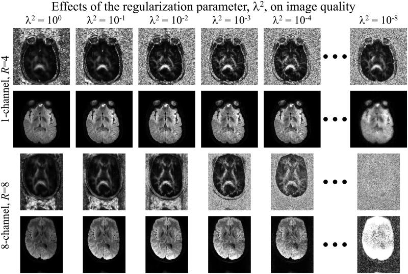
3. Adjusting the value of the regularization parameter, λ²

The effect of adjusting the regularization parameter, ι² from Eq. 2, was explored in Fig. 8. A slice acquired with acceleration R = 4 using a quadrature coil (described on line #3 in Table 1) and a similar slice acquired with acceleration R = 8 using an 8-channel coil (line #2 in Table 1) were both reconstructed using several different settings for ι². Both fractional anisotropy and diffusion-weighted images (b = 404 s/mm², 3^rd diffusion direction out of 6) are shown in Fig. 8 for each case. Increasing the value of ι² has a filtering effect on the results: The FA maps became more blurred spatially while noise content was decreased. Conversely, reducing the value of ι² tended to increase the noise content and to increase the spatial resolution in the FA maps, up to a point where λ² became simply too small for the proposed algorithm to perform properly. At such point, the low spatial frequency content may still have been correctly captured if the central k-space substitution scheme was employed, as was the case here, but the high spatial frequency content could not be properly reconstructed, thus leading to considerable blurring.

Fig. 8.

The effect of the regularization parameter, λ² from Eq. 2, was analyzed in the reconstruction of two different datasets: One with acceleration R = 4 and another with R = 8. An FA map and a diffusion-weighted image are shown in all cases. The noise content had a tendency to decrease with increasing λ² values, while both large and small values for λ² led to blurring. See text for more details.

A main difference between the R = 4 and the R = 8 cases presented in Fig. 8 had to do with voxel size, and thus SNR. Voxel size in the R = 4 case was 11.8 mm³, as opposed to only 2.95 mm³ (i.e., 4 times smaller) in the R = 8 case. When trying to select an optimum λ² set ting to be used for all R = 8 results, the noise-filtering effect associated with increasing λ² proved to be of considerable importance, and a relatively-large value of λ² = le-2 was se lected here. The value for λ² represents a compromise between spatial resolution in the FA maps, which benefits from λ² being small, and SNR, which benefits from λ² being large. For the larger-voxel R = 4 case, where SNR was less of a problem than in the R = 8 case, a small er setting for λ² could readily be considered and a value of λ² = le-3 was selected. For the intermediate R = 6 cases, associated here with a 5.25 mm³ voxel size, an intermediate setting of λ² = 5e-3 was chosen. While finding an optimum value for λ² for every given scan and de fining criteria for optimality would prove a challenging task, the results from Fig. 8 suggest that precisely tuning the value of λ² might be associated with only modest gains, and that identifying the correct order of magnitude (as shown in Fig. 8) might well suffice in practice.

4. DWI results

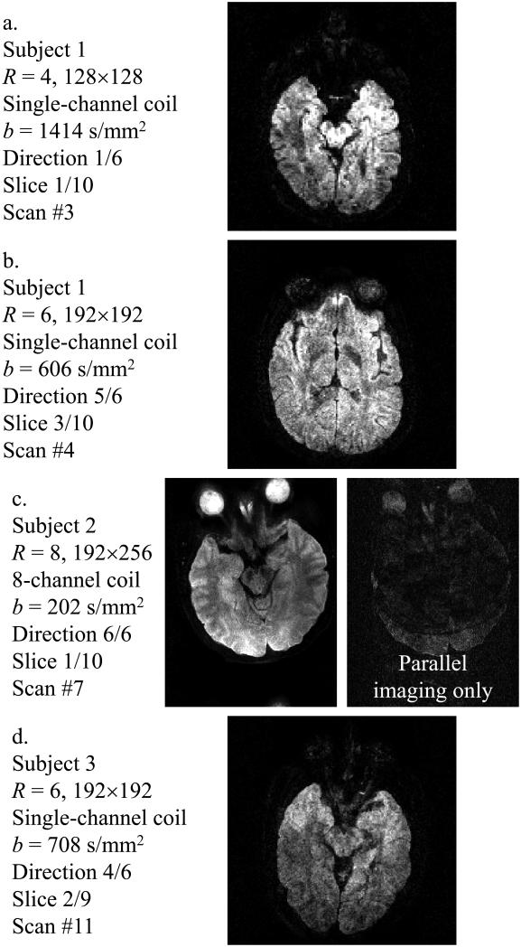
Figure 9 shows examples of diffusion-weighted images reconstructed using the present method. Considerable acceleration, ranging from R = 4 to R = 6, could be obtained even without involving parallel imaging, using a single-channel coil (Figs 9a, b and d). Results with R = 8 are shown in Fig. 9c alongside a parallel-imaging comparison. Results in Fig. 9 represent a collection of different acceleration factors R (4, 6 or 8), for single-channel as well as 8-channel coils and for different b-values ranging from 202 to 1414 s/mm². Figure 10 shows all four b-values that were reconstructed for scan #10 in Table 1 (slice #2 out of 9 and diffusion-encoding direction #4 out of 6), along with the corresponding FA map. It may be noted from Figs 9 and 10 that the proposed algorithm proved very effective at removing aliasing artifacts, and generated images of improved quality compared to parallel imaging alone.

Fig. 9.

Examples of diffusion-weighted images reconstructed using the proposed method. The subject number, acceleration factor R, matrix size, number of receiver elements, b-value, diffusion-encoding direction, slice number and entry number in Table 1 are provided for each example.

Fig. 10.

All four diffusion-weighted images reconstructed for scan #10 from Table 1 are shown here (slice #2 out of 9, diffusion-encoding direction #4 out of 6), along with the corresponding FA map.

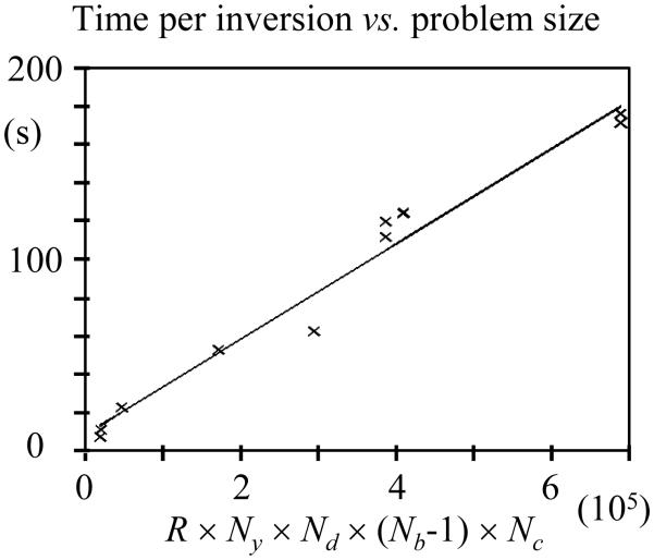
Information about reconstruction time is provided in Fig. 11. The processing time for all y locations at a given (x,z) location is plotted against R × N_y × N_d × (N_b-1) × N_c, for all results listed in Table 1. Through the linear fit in Fig. 11, the processing time for any given (x,z) location could be approximated as (m × R × N_y × N_d × (N_b-1) × N_c + 8.54 s), where the slope m is equal to 2.46×10^-4 s. For example, using this relationship, the processing time for all N_x × N_y × N_z spatial locations for the R = 6 case described on line 6 of Table 1 (N_x = 192, N_y = 192, N_z = 9, N_d =6, N_b = 8 and N_c = 8) would be approximated at 50 hr while it was actually measured at 53 hr and 4 min. Further optimization of the reconstruction code and/or using a computer system with more processors might, of course, very much reduce reconstruction time. Such improvements would reduce the value for the slope m in Fig. 11, but the relationship described above between processing time and other acquisition parameters would be expected to remain otherwise mostly unchanged. The fact that reconstruction time increased only linearly with the overall size of the acquired dataset, rather than more rapidly, is considered a very good sign in terms of the method’s overall practicality.

Fig. 11.

Reconstruction time for all y locations at a given x-z location was found to increase roughly linearly with (R × N_y × N_d × (N_b-1) × N_c), with a slope of m = 2.46×10^-4 s in the present implementation.

5. Tensor-imaging, kurtosis and fiber-crossing results

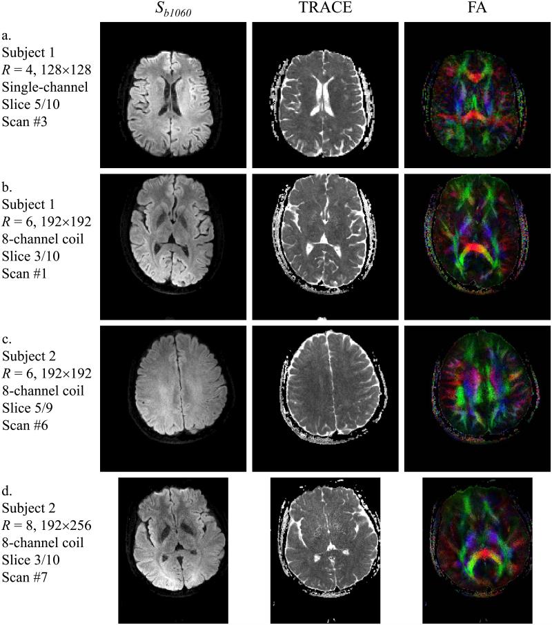
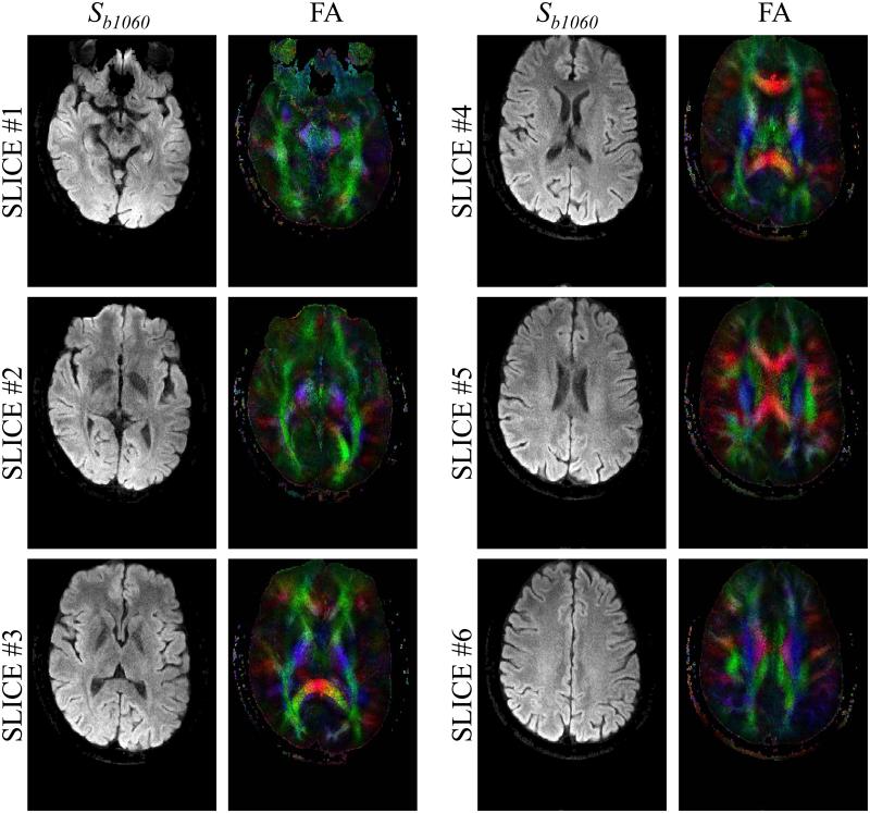
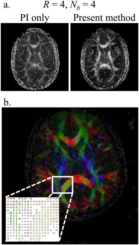
Tensor-imaging results are presented in Figs 12, 13 and 14. In Fig. 12, diffusion images with all-directions combined for b = 1060 s/mm² are presented in the first column, labeled S_b1060, while the trace and color-rendered fractional anisotropy are presented in the second and third columns. As in Fig. 9, results are shown for different acceleration factors (4, 6 and 8) and for the two different types of coils used here (8- and single-channel). In Fig. 13, results for the first 6 slices of scan #2 from Table 1 are shown. It may be noted from Fig. 13 that as expected from reducing the echo-train length, fairly good geometric fidelity was obtained even near the sinuses and ear canal. Reconstruction results from parallel imaging only and from the present method are compared in Fig. 14a for a case with R = 4 (N_b = 4, first 4 b-values from scan #9 in Table 1, slice 5/10). As the two results in Fig. 14a were reconstructed from the same acquired data, the geometric fidelity is the same in both cases; however an R = 4 setting proved beyond what could readily be achieved with our phased-array coil and parallel imaging alone, leading to a lower-quality FA map compared to that achieved using the proposed approach (see Fig. 14a).

Fig. 12.

Examples of diffusion tensor results are presented. For each case, the subject number, acceleration factor R, matrix size, number of receiver elements, slice number and entry number in Table 1 are provided. See text for more details.

Fig. 13.

The first (most inferior) six slices for one given scan are shown here (scan #2 from Table 1, R = 8, matrix size = 192×256, 8-channel coil). It may be noted that good geometric fidelity was obtained even for slice #1, located closest to the sinuses.

Fig. 14.

a) A 4-fold accelerated dataset was reconstructed using parallel-imaging only and using the proposed method (N_b = 4, the 4 first b-values from scan #9 in Table 1 were used here). b) The 100-direction dataset from entry #5 in Table 1 was reconstructed so that fiber crossings could be identified and mapped. Results from an ROI are shown and can be compared to the corresponding FA map.

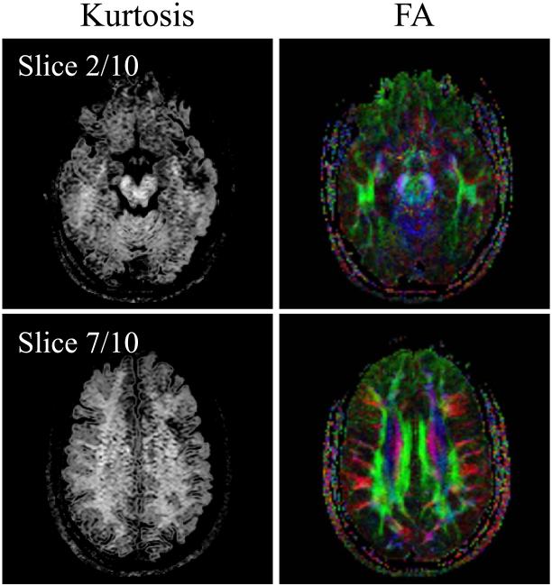
Reconstruction involving a Funk-Radon transform was applied to the N_d = 100 data described by entry #5 in Table 1, to resolve fiber crossings, and results are shown in Fig. 14b overlaid on an FA map. Kurtosis analysis (17) was applied to the data described by entry #9 in Table 1, and results are shown in Fig. 15. Overall, results from Figs 12-15 demonstrate that diffusion-weighted images reconstructed using the proposed method can be readily reconstructed using a variety of common and widely-available diffusion-imaging models and algorithms.

Fig. 15.

The data from entry #9 in Table 1 were reconstructed using both a kurtosis model and a mono-exponential tensor model. Kurtosis and fractional anisotropy results are shown side-by-side for an inferiorly-located and a mid-brain slice.

Discussion

A multi-shot motion-compensated acceleration method was proposed for DWI applications. As compared to non-accelerated single-shot methods, the present approach allows a reduction in the length of the echo train and, accordingly, a reduction in geometrical distortions. As compared to non-accelerated multi-shot methods, it allows a reduction in scan time at no cost in terms of geometrical fidelity. A key characteristic of the proposed method is how thoroughly the navigator signal gets utilized. As can be seen in Fig. 6, the navigator signal gives rise to a phase term employed for motion-correction purposes, a regularization magnitude term, an initial guess for the iterative solver and, optionally, it can be used for direct substitution of the central k-space region. Acceleration factors up to 6 and 8 have been obtained here without and with the inclusion of parallel imaging, respectively. While acceleration factors beyond 8 could probably have been obtained, the small improvements in geometric fidelity associated with further increasing acceleration might not have been worth their associated SNR cost. In other words, the maximum 8-fold acceleration used here was limited more by how much acceleration we could usefully employ in our present 2D multi-shot EPI implementation rather than by any actual acceleration limit of the proposed method itself.

Many different diffusion-encoding schemes have been proposed over the years, whereby a number of diffusion-encoded images are acquired using different b-values and/or diffusion directions. Most of the results presented here involved one particular Cartesian scheme, whereby the sampled b-values were linearly distributed between b ≈ 0 and some maximum value, b_max, and six different diffusion directions were sampled for each b-value. In contrast, results were also presented that involved acquiring a single non-zero b-value and many more diffusion directions. In principle at least, the present acceleration method does not impose any clear constraints on N_b and N_d, and any practically-achievable values could potentially be used. But intuitively, the bigger N_b ×N_d gets while keeping N_b ≈ N_d, the greater the area in k_b-k_d space that can be exploited toward the safe disposal of aliased signals, and the better the proposed method can be expected to perform.

A multiple b-value sampling scheme, as used for most of the results presented here, may often be desirable as the diffusion signal decay in biological tissues cannot be accurately described using a mono-exponential model. The proposed acceleration method makes no assumptions about decay, non-exponential decay is preserved through the reconstruction of a multiple b-value dataset, and processing tools such as multi-exponential fitting or kurtosis analysis can be applied on the reconstructed DWI results (e.g., see kurtosis results in Fig. 15). In a special case where the acceleration factor, R, would be equal to the number of b-factors minus 1, (N_b – 1), the present method as currently implemented would be no faster than a non-accelerated acquisition with N_b = 2. As compared to such a minimum-N_b acquisition, the present method can allow the number of b-values to be increased from 2 to (R + 1) while keeping scan time and geometric fidelity essentially unchanged. Sampling more b-values may help appropriately capture a wider range of diffusion coefficients, and/or potentially enable more elaborate fitting procedures to assess the non-monoexponential diffusion signal decay properties of water in tissues (19, 20). On the other hand, even in cases where a single non-zero b-value is sampled, the proposed scheme may still be utilized to help reduce spatial distortion.

The proposed method is meant as an adjunct to existing acceleration methods such as parallel imaging, partial-Fourier imaging and compressed sensing. Parallel imaging is typically used to help reduce the echo-train length and the spatial distortion from EPI sequences, while partial-Fourier imaging also reduces echo-train length but does not help in terms of spatial distortions (unless it is implemented along the k_x direction instead of k_y, which would be unusual for DWI applications). These methods do not reduce the number of diffusion-encoded images that need to be acquired, but rather the number of k-space lines acquired for each one of these images. Compressed sensing, on the other hand, can be used to reduce the number of acquired diffusion-encoded images, and thus reduce the overall scan time. Compressed sensing is not typically used to reduce the number of k_y lines acquired with a 2D EPI sequence, as doing so would require randomizing the size of the EPI gradient blips that perform the spatial encoding along the y direction, potentially causing artifacts related to eddy currents. It should be possible to combine all of these methods for added effect, whereby the EPI echo-train length would be reduced by a combination of our proposed method, parallel imaging and partial-Fourier imaging, while scan time and the number of sampled diffusion-encoded directions would be reduced by compressed sensing. Both fast imaging and good geometric fidelity might thus be simultaneously attained, but doing so is considered beyond the scope of the present work.

Conclusions

An accelerated motion-corrected diffusion imaging method was introduced that achieves good image quality at relatively high acceleration factors. Up to 8-fold and 6-fold acceleration was achieved here with and without including parallel imaging, respectively. A main characteristic of the method is how thoroughly the navigator-echo data are employed, especially for motion correction and regularization purposes.

References

- 1.Atkinson D, Counsell S, Hajnal JV, Batchelor PG, Hill DL, Larkman DJ. Nonlinear phase correction of navigated multi-coil diffusion images. Magn Reson Med. 2006;56(5):1135–1139. doi: 10.1002/mrm.21046. [DOI] [PubMed] [Google Scholar]
- 2.Anderson AW, Gore JC. Analysis and correction of motion artifacts in diffusion weighted imaging. Magn Reson Med. 1994;32(3):379–387. doi: 10.1002/mrm.1910320313. [DOI] [PubMed] [Google Scholar]
- 3.Butts K, de Crespigny A, Pauly JM, Moseley M. Diffusion-weighted interleaved echo-planar imaging with a pair of orthogonal navigator echoes. Magn Reson Med. 1996;35(5):763–770. doi: 10.1002/mrm.1910350518. [DOI] [PubMed] [Google Scholar]
- 4.Miller KL, Pauly JM. Nonlinear phase correction for navigated diffusion imaging. Magn Reson Med. 2003;50(2):343–353. doi: 10.1002/mrm.10531. [DOI] [PubMed] [Google Scholar]
- 5.Holdsworth SJ, Skare S, Newbould RD, Bammer R. Robust GRAPPA-accelerated diffusion-weighted readout-segmented (RS)-EPI. Magn Reson Med. 2009;62(6):1629–1640. doi: 10.1002/mrm.22122. PMCID:PMC2904969. [DOI] [PMC free article] [PubMed] [Google Scholar]
- 6.Jeong HK, Gore JC, Anderson AW. High-resolution human diffusion tensor imaging using 2-D navigated multishot SENSE EPI at 7 T. Magn Reson Med. 2012 doi: 10.1002/mrm.24320. PMCID:PMC3424313. [DOI] [PMC free article] [PubMed] [Google Scholar]
- 7.Porter DA, Heidemann RM. High resolution diffusion-weighted imaging using readout-segmented echo-planar imaging, parallel imaging and a two-dimensional navigator-based reacquisition. Magn Reson Med. 2009;62(2):468–475. doi: 10.1002/mrm.22024. [DOI] [PubMed] [Google Scholar]
- 8.Engstrom M, Skare S. Diffusion-weighted 3D multislab echo planar imaging for high signal-to-noise ratio efficiency and isotropic image resolution. Magn Reson Med. 2013 doi: 10.1002/mrm.24594. [DOI] [PubMed] [Google Scholar]
- 9.Frank LR, Jung Y, Inati S, Tyszka JM, Wong EC. High efficiency, low distortion 3D diffusion tensor imaging with variable density spiral fast spin echoes (3D DW VDS RARE) Neuroimage. 2010;49(2):1510–1523. doi: 10.1016/j.neuroimage.2009.09.010. PMCID:PMC2791091. [DOI] [PMC free article] [PubMed] [Google Scholar]
- 10.Tsao J, Boesiger P, Pruessmann KP. k-t BLAST and k-t SENSE: dynamic MRI with high frame rate exploiting spatiotemporal correlations. Magn Reson Med. 2003;50(5):1031–1042. doi: 10.1002/mrm.10611. [DOI] [PubMed] [Google Scholar]
- 11.Menzel MI, Tan ET, Khare K, Sperl JI, King KF, Tao X, Hardy CJ, Marinelli L. Accelerated diffusion spectrum imaging in the human brain using compressed sensing. Magn Reson Med. 2011;66(5):1226–1233. doi: 10.1002/mrm.23064. [DOI] [PubMed] [Google Scholar]
- 12.Hansen PC. Direct regularization methods. Rank-deficient and discrete ill-posed problems. Siam Press; Philadelphia, USA: 1998. p. 100. [Google Scholar]
- 13.Madore B, Glover GH, Pelc NJ. Unaliasing by Fourier-encoding the overlaps using the temporal dimension (UNFOLD), applied to cardiac imaging and fMRI. Magn Reson Med. 1999;42:813–828. doi: 10.1002/(sici)1522-2594(199911)42:5<813::aid-mrm1>3.0.co;2-s. [DOI] [PubMed] [Google Scholar]
- 14.Chao TC, Chung HW, Hoge WS, Madore B. A 2D MTF approach to evaluate and guide dynamic imaging developments. Magn Reson Med. 2010;63(2):407–418. doi: 10.1002/mrm.22219. [DOI] [PMC free article] [PubMed] [Google Scholar]
- 15.Wu YC, Alexander AL. Hybrid diffusion imaging. Neuroimage. 2007;36(3):617–629. doi: 10.1016/j.neuroimage.2007.02.050. PMCID:PMC2428345. [DOI] [PMC free article] [PubMed] [Google Scholar]
- 16.Wedeen VJ, Hagmann P, Tseng WY, Reese TG, Weisskoff RM. Mapping complex tissue architecture with diffusion spectrum magnetic resonance imaging. Magn Reson Med. 2005;54(6):1377–1386. doi: 10.1002/mrm.20642. [DOI] [PubMed] [Google Scholar]
- 17.Jensen JH, Helpern JA, Ramani A, Lu H, Kaczynski K. Diffusional kurtosis imaging: the quantification of non-gaussian water diffusion by means of magnetic resonance imaging. Magn Reson Med. 2005;53(6):1432–1440. doi: 10.1002/mrm.20508. [DOI] [PubMed] [Google Scholar]
- 18.Lustig M, Donoho D, Pauly JM. Sparse MRI: The application of compressed sensing for rapid MR imaging. Magn Reson Med. 2007;58(6):1182–1195. doi: 10.1002/mrm.21391. [DOI] [PubMed] [Google Scholar]
- 19.Mulkern RV, Gudbjartsson H, Westin CF, Zengingonul HP, Gartner W, Guttmann CR, Robertson RL, Kyriakos W, Schwartz R, Holtzman D, Jolesz FA, Maier SE. Multi-component apparent diffusion coefficients in human brain. NMR Biomed. 1999;12(1):51–62. doi: 10.1002/(sici)1099-1492(199902)12:1<51::aid-nbm546>3.0.co;2-e. [DOI] [PubMed] [Google Scholar]
- 20.Pang Y, Turkbey B, Bernardo M, Kruecker J, Kadoury S, Merino MJ, Wood BJ, Pinto PA, Choyke PL. Intravoxel incoherent motion MR imaging for prostate cancer: An evaluation of perfusion fraction and diffusion coefficient derived from different b-value combinations. Magn Reson Med. 2012 doi: 10.1002/mrm.24277. PMCID:PMC3413736. [DOI] [PMC free article] [PubMed] [Google Scholar]