Integration of Sparse Multi-modality Representation and Anatomical Constraint for Isointense Infant Brain MR Image Segmentation

Abstract

Segmentation of infant brain MR images is challenging due to poor spatial resolution, severe partial volume effect, and the ongoing maturation and myelination process. During the first year of life, the brain image contrast between white and gray matters undergoes dramatic changes. In particular, the image contrast inverses around 6–8 months of age, where the white and gray matter tissues are isointense in T1 and T2 weighted images and hence exhibit the extremely low tissue contrast, posing significant challenges for automated segmentation. In this paper, we propose a general framework that adopts sparse representation to fuse the multi-modality image information and further incorporate the anatomical constraints for brain tissue segmentation. Specifically, we first derive an initial segmentation from a library of aligned images with ground-truth segmentations by using sparse representation in a patch-based fashion for the multi-modality T1, T2 and FA images. The segmentation result is further iteratively refined by integration of the anatomical constraint. The proposed method was evaluated on 22 infant brain MR images acquired at around 6 months of age by using a leave-one-out cross-validation, as well as other 10 unseen testing subjects. Our method achieved a high accuracy for the Dice ratios that measure the volume overlap between automated and manual segmentations, i.e., 0.889±0.008 for white matter and 0.870±0.006 for gray matter.

1 Introduction

The first year of life is the most dynamic phase of the postnatal human brain development, with rapid tissue growth and the development of a wide range of cognitive and motor functions (Fan et al., 2011; Paus et al., 2001; Zilles et al., 1988). Accurate tissue segmentation of infant brain MR images into white matter (WM), gray matter (GM) and cerebrospinal fluid (CSF) in this stage is of great importance in studying and measuring the normal and abnormal early brain development (Li et al., 2013a; Li et al., 2013b; Li et al., 2013c; Nie et al., 2012). It is well-known that the segmentation of infant brain MRI is considerably more difficult than that of the adult brain, due to the reduced tissue contrast (Weisenfeld and Warfield, 2009), increased noise, severe partial volume effect (Xue et al., 2007), and ongoing white matter myelination (Gui et al., 2012; Weisenfeld and Warfield, 2009) in the infant brain images. Three distinct stages exist in the infant brain MR images, as shown in Fig. 1, with each stage having quite different white matter/gray matter contrast patterns (in chronological order) (Paus et al., 2001): (1) the infantile stage (≤ 5 months), in which the gray matter shows a higher signal intensity than the white matter in T1 images; (2) the isointense stage (6–12 months), in which the signal intensity of the white matter is increasing during the development due to the myelination and maturation process; in this stage, the gray matter has the lowest signal differentiation with the white matter in both T1 and T2 images; (3) the early adult-like stage (>12 months), where the gray matter intensity is much lower than that of the white matter in T1 images, similar to the pattern of tissue contrast in the adult MR images. Note that T2 images have the reversed tissue contrast patterns, in contrast to T1 images. Also, the appearance of exact isointense contrast varies across different brain regions due to the nonlinear brain development (Paus et al., 2001). The middle column of Fig. 1 shows examples of T1 and T2 images scanned at around 6 months of age. It can be observed that the intensities of voxels in gray matter and white matter are in the similar range (especially in the cortical regions), resulting in the lowest image contrast in the first year and hence the significant difficulties for tissue segmentation.

Fig. 1.

Illustration of three distinct stages in infant brain development, with each stage having quite different WM/GM contrast patterns in MR images. The corresponding tissue intensity distributions from T2-weighted MR images are shown in the bottom row, which indicates high overlap of WM and GM intensities in the isointenste stage.

As briefed in Table 1, although many methods have been proposed for infant brain MR image segmentation, most of them focused either on segmentation of the infant brain images in the infantile stage (≤ 5 months) or early adult-like stage (>12 months) by using a single T1 or T2 image or the combination of T1 and T2 images (Cardoso et al., 2013; Gui et al., 2012; Kim et al., 2013; Leroy et al., 2011; Nishida et al., 2006; Shi et al., 2010a; Song et al., 2007; Wang et al., 2011; Wang et al., 2013c; Weisenfeld et al., 2006a, b; Weisenfeld and Warfield, 2009; Xue et al., 2007), where images have the relatively distinguishable contrast between white matter and gray matter. However, most of the existing methods (Cardoso et al., 2013; Prastawa et al., 2005; Shi et al., 2010a; Wang et al., 2011; Xue et al., 2007) typically assume that each tissue class throughout the entire image can be modeled by a single Gaussian distribution or the mixture of Gaussian distributions. This assumption is valid for the images acquired from the infantile stage, however, in the isointenste stage, the distributions of WM and GM are largely overlapped due to the ongoing maturation and myelination process, as shown in Fig. 1. Therefore, these methods cannot achieve reasonable segmentation on the isointense infant images. Thus, it is necessary to use more image modalities, such as fractional anisotropy (FA) images (Liu et al., 2007; Wang et al., 2012b; Yap et al., 2011), and a general framework for effectively utilizing and fusing multi-modality information is highly desired.

Table 1.

A brief summary of existing methods for infant brain MR image segmentation.

Methods	Modality	Age at scan			Longitudinal?
		Infantile	Isointense	Early adult-like
(Prastawa et al., 2005)	T1, T2	✓			No
(Weisenfeld et al., 2006a)	T1, T2	✓			No
(Weisenfeld et al., 2006b)	T1, T2	✓			No
(Nishida et al., 2006)	T1	✓			No
(Xue et al., 2007)	T2	✓			No
(Song et al., 2007)	T2	✓			No
(Anbeek et al., 2008)	T2, IR	✓			No
(Weisenfeld and Warfield, 2009)	T1, T2	✓			No
(Shi et al., 2010a)	T1, T2	✓		✓	Yes
(Shi et al., 2010b)	T2	✓			No
(Shi et al., 2010c)	T1, T2	✓	✓	✓	Yes
(Wang et al., 2011)	T2	✓			No
(Shi et al., 2011a)	T1, T2	✓			No
(Leroy et al., 2011)	T2	✓			No
(Gui et al., 2012)	T1, T2	✓			No
(Wang et al., 2012b)	T1, T2, FA	✓	✓	✓	Yes
(Kim et al., 2013)	T1			✓	No
(He and Parikh, 2013)	T2, PD	✓			No
(Wang et al., 2013c)	T1, T2	✓		✓	Yes
(Cardoso et al., 2013)	T1	✓			No
(Wang et al., 2014)	T2	✓			No
The proposed method	T1, T2, FA	✓	✓	✓	No

In (Shi et al., 2011b), infant brain atlases from neonatal to 1- and 2-years old were proposed for guiding the tissue segmentation. A dynamic 4D probabilistic atlas of the developing brain has been proposed in (Kuklisova-Murgasova et al., 2011). However, this 4D atlas only cover the developing brain between 29 and 44 weeks gestational age. Few studies have addressed the difficulties in segmentation of the isointense infant images. Shi et al. (Shi et al., 2010c) first proposed a 4D joint registration and segmentation framework for the segmentation of infant MR images in the first year of life. In this method, longitudinal images in both infantile and early adult-like stages were used to guide the segmentation of images in the isointense stage. A similar strategy was later adapted in (Wang et al., 2012b). The major limitation of these methods is that they fully depend on the availability of longitudinal datasets (Kim et al., 2013). Due to the fact that the majority of infant images have no longitudinal follow-up, a standalone method working for the cross-sectional single-time-point image is highly desired.

To segment the single-time-point isointense infant brain images, previous pure appearance-driven segmentation methods are likely to generate topological or anatomical defects in brain segmentation (e.g., holes and handles in the white matter surface). Although the defects, such as holes, may be corrected by adding the surface area constraints as in the level set based methods (Wang et al., 2011; Wang et al., 2013c), these methods intend to penalize the high curvatures, which may result in under-segmentation in some sharp cortical regions. On the other hand, there are many topological correction methods (Bazin and Pham, 2005; Fischl et al., 2001; Han et al., 2004; Segonne et al., 2007; Shattuck and Leahy, 2001), which can generate accurate topological corrections on cortical surfaces. Although these methods didn’t tend to smooth out the high curvature areas, their topological correction results are not always the desired ones (Segonne et al., 2007), e.g., the sharp peaks (usually due to noise) are topologically correct, but are anatomically incorrect (Yotter et al., 2011). To overcome these limitations, it is necessary to incorporate brain anatomical information into the segmentation procedure.

In addition, most of the previous methods perform segmentation in a voxel-by-voxel fashion. Based on the fact that image patches could capture more anatomical information than a single voxel, recently, patch-based methods (Bai et al., 2013; Coupé et al., 2012a; Coupé et al., 2012b; Coupé et al., 2011; Eskildsen et al., 2012; Rousseau et al., 2011) have been proposed for label fusion and segmentation. Their main idea is to allow for integration of multiple candidates (usually in the neighborhood) from each template based on non-local means (Buades et al., 2005). Different from multi-atlas based label fusion algorithms (Asman and Landman, 2013; Langerak et al., 2010; Sabuncu et al., 2010; Wang et al., 2012a; Warfield et al., 2004), which require accurate non-rigid image registration, these patch-based methods are less dependent on the accuracy of registration. This technique has been successfully validated on brain labeling (Rousseau et al., 2011) and hippocampus segmentation (Coupé et al., 2011) with promising results.

Motivated by the fact that many classes of signals, such as audio and images, have naturally sparse representations with respect to each other, sparse representation has been widely and successfully used in many fields (Gao et al., 2012; Liao et al., 2013; Tong et al., 2012; Wright et al., 2009; Zhang et al., 2011b), such as image denoising (Elad and Aharon, 2006; Mairal et al., 2008b), image in-painting (Fadili et al., 2009), image recognition (Mairal et al., 2008a; Winn et al., 2005), and image super-resolution (Yang et al., 2010), achieving the state-of-the-art performance. In this paper, we propose a general framework that adopts sparse representation to fuse the multi-modality image information and incorporate the anatomical constraints for brain segmentation. Specifically, we first construct a library consisting of a set of multi-modality images from the training subjects and their corresponding ground-truth segmentations. Multi-modality library consists of T1, T2 and fractional anisotropy (FA) images (the third column of Fig. 2), which provide rich information of major WM bundles (Liu et al., 2007), is used to deal with the problem of insufficient tissue contrast (Paus et al., 2001). To segment a testing brain image, each patch is sparsely represented by the training library patches. The initial segmentation is thus obtained based on the derived sparse coefficients. To enforce the anatomical correctness of the segmentation, the initial segmentation will be refined with further consideration of the patch similarities between the segmented testing image and the manual segmentations (ground-truth) in the library images. By iterative refinement, we can obtain anatomically more reasonable segmentation. In summary, the major contributions of our work include:

Fig. 2.

Three randomly selected subjects, along with their corresponding manual segmentation results.

1. We apply the patch-based sparse representation into the segmentation of the isointense infant MR image in a multi-modality fashion.

2. We integrate the anatomical constraint into the sparse representation to further improve the segmentation.

Note that partial results in this paper were reported in our recent conference paper (Wang et al., 2013a). The remainder of this paper is organized as follows. The proposed method is introduced in Section 2. The experimental results are then presented in Section 3, followed by the discussion and conclusion in Section 4.

2 Method

2.1 Subjects and data acquisition

A total of 22 healthy infant subjects (12 males/10 females) were recruited, and scanned at 27±0.9 postnatal weeks. MR images were acquired on a Siemens head-only 3T scanner with a circular polarized head coil. Infants were scanned unsedated while asleep, fitted with ear protection and with their heads secured in a vacuum-fixation device. T1-weighted images were acquired with 144 sagittal slices using parameters: TR/TE=1900/4.38ms, flip angle=7°, resolution=1×1×1 mm³. T2-weighted images were obtained with 64 axial slices: TR/TE=7380/119ms, flip angle=150° and resolution=1.25×1.25×1.95 mm³. Diffusion weighted images consist of 60 axial slices: TR/TE=7680/82ms, resolution=2×2×2 mm³, 42 non-collinear diffusion gradients, and b=1000s/mm². Seven non-diffusion-weighted reference scans were also acquired. The diffusion tensor images were reconstructed and the respective FA images were computed. Data with motion artifacts was discarded and a rescan was made when possible. This study has been approved by institute IRB and the written informed consent forms were obtained from parents.

2.2 Image preprocessing and library construction

T2 and FA images were linearly aligned onto their corresponding T1 images and further resampled into a 1×1×1 mm³ resolution. Specifically, the T2 image of each subject was first rigidly aligned to the T1 image, and then the FA image was rigidly aligned to the warped T2 image. The idea is that, since those multi-modality images are from the same subject, they share the same brain anatomy, and thus allowed to be accurately aligned with rigid registration. Standard preprocessing steps were performed before segmentation, including skull stripping (Shi et al., 2012), intensity inhomogeneity correction (Sled et al., 1998), and removal of the cerebellum and brain stem by using in-house tools. Ideally, one would use MR images with manual segmentations to create the library, which, however, is heavily time-consuming. To generate the ground-truth segmentations, we took a practical approach by first generating an initial reasonable segmentation by using a publicly available software iBEAT (Dai et al., 2013)(http://www.nitrc.org/projects/ibeat/). Then, manual editing was performed by an experienced rater to correct segmentation errors and geometric defects by using ITK-SNAP (Yushkevich et al., 2006) (www.itksnap.org), with the help of surface rendering. For example, if there is a hole/handle in the surface, the rater will first localize the related slices, and then check the segmentation on the T1, T2 and FA images to finally determine whether to fill the hole or cut the handle. The detailed instruction of manual segmentation can be found http://www.itksnap.org/. It takes around 3 hours to complete the manual editing for each subject. The intra-rater reliability (4 repeats) for WM, GM and CSF is 0.934, 0.925, and 0.920, respectively, in terms of Dice ratio. Fig. 2 shows three randomly selected subjects, along with their corresponding manual segmentations.

2.3 Deriving initial segmentation by sparse representation

To segment a testing image I = {I_T1, I_T2, I_FA}, N template images sets ${\mathit{I}}^i=\{I_{T1}^i,I_{T2}^i,I_{FA}^i\}$ and their corresponding segmentation maps Lⁱ(i = 1, …, N) are first nonlinearly aligned onto the space of the testing image using Diffeomorphic Demons (Vercauteren et al., 2009), based on T1 images. There are Then, for each voxel x in each modality image of the testing image I, its intensity patch (taken from w × w × w neighborhood) can be represented as a w × w × w dimensional column vector. By taking the T1 image as an example, the T1 intensity patch can be denoted as m_T1(x). Furthermore, its patch dictionary can be adaptively built from all N aligned templates as follows. First, let (x) be the neighborhood of voxel x in the i-th template image $I_{T1}^i$, with the neighborhood size as w_p × w_p × w_p. Then, for each voxel y ∈ (x), we can obtain its corresponding patch from the i-th template, i.e., a w × w × w dimensional column vector ${\mathit{m}}_{T1}^i(y)$. By gathering all these patches from w_p × w_p × w_p neighborhoods of all N aligned templates, we can build a dictionary matrix D_T1, where each patch is represented by a column vector and normalized to have the unit ℓ2 norm (Cheng et al., 2009; Wright et al., 2010). In the same manner, we can also extract T2 intensity patch m_T2(x) and FA intensity patch m_FA(x) from the testing image I and further build the respective dictionary matrices D_T2 and D_FA from the aligned templates. Let M(x) = [m_T1(x); m_T2(x); m_FA(x)] be the testing multi-modality patch and ${\mathit{M}}^i(y)=\left[{\mathit{m}}_{T1}^i(y);{\mathit{m}}_{T2}^i(y);{\mathit{m}}_{FA}^i(y)\right]$ be the i–th template multi-modality patch in the dictionary. To represent the patch M(x) by the dictionaries $\mathit{D}(x)\stackrel{\text{def}}{=}[{\mathit{D}}_{T1};{\mathit{D}}_{T2};{\mathit{D}}_{FA}]$, its coefficients vector α could be estimated by many coding schemes, such as sparse coding (Wright et al., 2009; Yang et al., 2009) and locality-constrained linear coding (Wang et al., 2010). Here, we employ sparse coding scheme (Wright et al., 2009; Yang et al., 2009), which is robust to the noise and outlier, to estimate the coefficient vector α by minimizing a non-negative Elastic-Net problem (Zou and Hastie, 2005),

$$\underset{\begin{array}{c}\mathit{\alpha }\\ \mathit{\alpha }\ge \mathbf{0}\end{array}}{min}\underset{\text{Intensity}\text{patch}\text{constraint}}{\underbrace{\sum {\Vert \mathit{M}(x)-\mathit{D}(\mathit{x})\mathit{\alpha }\Vert }_2^2}}+{\lambda }_1{\Vert \mathit{\alpha }\Vert }_1+{\lambda }_2{\Vert \mathit{\alpha }\Vert }_2^2$$ (1)

In the above Elastic-Net problem, the first term is the data fitting term based on the intensity patch similarity, and the second term is the ℓ1 regularization term which is used to enforce the sparsity constraint on the reconstruction coefficients α, and the last term is the ℓ2 smoothness term to enforce the coefficients to be similar for the similar patches. Eq. (1) is a convex combination of ℓ1 lasso (Tibshirani, 1996) and ℓ2 ridge penalty, which encourages a grouping effect while keeping a similar sparsity of representation (Zou and Hastie, 2005). In our implementation, we use the LARS algorithm (Efron et al., 2004), which was implemented in the SPAMS toolbox (http://spams-devel.gforge.inria.fr), to solve the Elastic-Net problem. Each element of the sparse coefficient vector α, i.e., αⁱ(y), reflects the similarity between the target patch M(x) and each patch Mⁱ(y) in the patch dictionary. Based on the assumption that similar patches should share similar labels, we use the sparse coefficients α to estimate the probability of the voxel x belonging to the j-th tissue, j ∈ {WM, GM, CSF}, i.e.,

$$P_j(x)=\sum _i\sum _{y\in {\mathcal{N}}^i(x)}{\alpha }^i(y){\delta }_j\left(L^i(y)\right)$$ (2)

where Lⁱ(y) is the segmentation label (WM, GM, or CSF) for voxel y in the i-th template image, and δ_j(Lⁱ(y)) is defined as

$${\delta }_j\left(L^i(y)\right)=\{\begin{array}{c}1,L^i(y)=j\\ 0,L^i(y)\ne j\end{array}$$ (3)

Finally, P_j(x) is normalized to ensure Σ_j P_j(x) = 1. The third row of Fig. 3 shows an example of the estimated probability maps of a testing image, with the original T1, T2 and FA images shown in the first row. To convert from the soft probability map to the hard segmentation, the label of the voxel x is determined using the maximum a posteriori (MAP) rule.

Fig. 3.

Tissue probability maps estimated by the proposed method without and with sparse constraint, without and with the anatomical constraint.

To demonstrate the advantage of enforcing the sparsity, we set λ₁ =0, which means that the all reference patches in the dictionary could contribute to the tissue probability estimation, regardless of their similarity to the testing patch. Consequently, the reference patches from the unrelated tissues may have contribution and thus mislead the estimation of tissue probability and finally the segmentation. In contrast, with the sparse constraint, most coefficients are set to be 0, with only a small number of reference patches (which share high similarity with the testing patch) having non-zero coefficients. In our experiments, we set the λ₁ =0.2 and selected typically 30 reference patches. For qualitative examination, we show the probability maps without the sparsity in the second row of Fig. 3. It can be clearly seen that, without the sparsity, the probability maps are fuzzy and unclear, especially for the WM/GM boundaries, as indicated by the green boxes. In contrast, the probability maps derived with the use of the sparse constraint are much sharper and accurate (see the third row of Fig. 3) and they can be considered as a subject-specific atlas. The quantitative comparisons between the results obtained without and with sparse constraint are provided in the third row of Fig. 5.

Fig. 5.

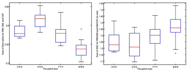
Influence of each parameter: patch size (1^st row), neighborhood size (2^nd row), weight for the ℓ1 norm (3^rd row), and weight for the ℓ2 norm (4^th row).

2.4 Imposing brain anatomical constraints into the segmentation

The tissue probability maps derived in the Section 2.3 are purely based on the intensity patch similarity using the sparse representation technique. However, due to the low tissue contrast, the reliability of the patch similarity could be limited, which may result in considerable artificial anatomical errors in the tissue probability maps. A typical example is shown in Fig. 4(a), where we can observe many undesired holes (green rectangles), incorrect connections (red rectangles), and inaccurate segmentations (blue rectangles).

Fig. 4.

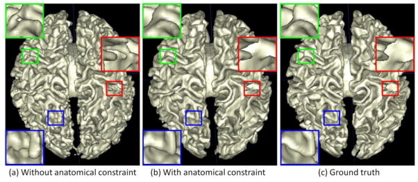
Comparison of WM surfaces reconstructed by the proposed method (a) without and (b) with the anatomical constraint, with the manual ground-truth segmentation in (c). The zoom-up view of each rectangular region is also provided.

Motivated by the success of sparse representation in image denoising (Elad and Aharon, 2006; Mairal et al., 2008b), we adopt sparse representation to incorporate the anatomical constraint into the segmentation. In the image denoising, given a noisy patch, sparse representation aims to select a small set of “clean” patches in the dictionary to reconstruct it. The reconstructed patch is used as the denoised patch. Following the similar idea, we can use sparse representation to correct the anatomical errors introduced in the segmentation. As the manual ground-truth segmentations of template images in the library are almost free of the anatomical errors after manual edition, we could expect that the incorporation of these segmentation results will largely reduce the potential anatomical errors. Specifically, we can extract the patch m_seg(x) from the tentative segmentation result of the testing image and also construct the segmentation patch dictionary D_seg(x) from all the segmented images in the library. Based on Eq. (1), we further incorporate the anatomical constraint to derive the refined tissue probability maps:

$$\underset{\begin{array}{c}\mathit{\alpha }\\ \mathit{\alpha }\ge 0\end{array}}{min}\underset{\text{Intensity}\text{patch}\text{constraint}}{\underbrace{\sum {\Vert \mathit{M}(x)-\mathit{D}(\mathit{x})\mathit{\alpha }\Vert }_2^2}}+\underset{\text{Anatomical}\text{constraint}}{\underbrace{\left\{v{\Vert {\mathit{m}}_{\mathit{seg}}(x)-{\mathit{D}}_{\mathit{seg}}(x)\mathit{\alpha }\Vert }_2^2\right\}}}+{\lambda }_1{\Vert \mathit{\alpha }\Vert }_1+{\lambda }_2{\Vert \mathit{\alpha }\Vert }_2^2$$ (4)

where v is the weight parameter for controlling the contribution of the anatomical constraint term. In the same way, we can use Eq. (2) to estimate new tissue probabilities, which will be iteratively refined by using Eq. (4) until convergence. An example of the probabilities derived with the anatomical constraint is shown in the fourth row of Fig. 3. Compared with the probability maps estimated without the anatomical constraint (the third row of Fig. 3), the new probability maps are more accurate since the discrete labels in the segmentation results can be less ambiguous than the intensity values in differentiating tissue types (Bai et al., 2013). Fig. 4(b) shows the WM surface with the anatomical constraint. Compared with the result obtained without the anatomical constraint (Fig. 4(a)), many geometric errors have been corrected.

3 Experimental results

In this section, the proposed method will be extensively evaluated on 22 infant subjects using leave-one-out cross-validation, and also on 10 additional testing subjects. Results of the proposed method are compared with the manual ground-truth segmentations, as well as other state-of-the-art methods.

3.1 Evaluation Metrics

In the following, we mainly employ Dice ratio to evaluate the segmentation accuracy, which is defined as:

$$DR=2\mid A\cap B\mid /(\mid A\mid +\mid B\mid )$$ (5)

where A and B are two segmentation results of the same image. We also evaluate the accuracy by measuring the average surface distance error (SDE), which is defined as:

$$\mathit{SDE}(A,B)=\frac{1}{2}\left(\frac{1}{n_A}{\sum }_{a\in \mathit{surf}(A)}\mathit{dist}(a,B)+\frac{1}{n_B}{\sum }_{b\in \mathit{surf}(B)}\mathit{dist}(b,A)\right)$$ (6)

where surf(A) is the surface of segmentation A, n_A is the total number of surface points in surf(A), and dist(a, B) is the nearest Euclidean distance from a surface point a to the surface B.

3.2 Impact of the parameters

Values for the parameters in our proposed method were determined via cross-validation on all training templates, according to the parameter settings described in (Bach et al., 2012). During parameter optimization, when optimizing a certain parameter, the other parameters were set to their own fixed values. We first study the impact of patch size on segmentation accuracy. Both the best Dice ratios and average SDE were obtained when using a patch size of 5×5×5, as shown in the first row of Fig. 5. The optimal patch size is related to the complexity of the anatomical structure (Coupé et al., 2011; Tong et al., 2013). On the other hand, the optimal search neighborhood size is related with the anatomical variability after registration (Coupé et al., 2011; Tong et al., 2013). Similarly, the impact of the sparse parameter λ₁ is shown in the third row of Fig. 5. It can be observed that, if there is no sparse constraint (λ₁ = 0), which means that all reference patches in the dictionary could contribute to the estimation of tissue probability, regardless of their similarity to the testing patch, the Dice ratios are quite low and the surface distance errors are also very large. When λ₁ > 0, the accuracy is greatly improved, with the best accuracy obtained with λ₁ = 0.2. All these demonstrates the importance of using the sparsity in tissue segmentation. On the other hand, there is no significant difference among λ₁ = [0.01 0.1 0.2 0.5], which indicates that our proposed method is robust to the value of λ₁. Based on (Bach et al., 2012), since we want to achieve the sparsity on selection of reference patches, we often set λ₂ as a small positive value. In our experiments, we test λ₂ =[0.001, 0.01, 0.1], and obtained the optimal one as 0.01. Note that the above range for each parameter was empirically chosen in our experiments, which could lead to local minimum results.

3.3 Number of the templates

The last important parameter of the proposed method is the number of templates. Fig. 6 shows the Dice ratios as a function of different number of templates. As expected, increasing the number of templates generally improves the segmentation accuracy, as the average Dice ratio increases from 0.85 (N = 1) to 0.89 (N = 20) for WM, 0.82 (N = 1) to 0.87 (N = 20) for GM, and 0.75 (N = 1) to 0.86 (N = 20) for CSF. Increasing the number of templates seems to make the segmentations more consistent as reflected by the reduced standard deviation from 0.02 (N = 1) to 0.008 (N = 20) for WM, 0.02 (N = 1) to 0.006 (N = 20) for GM, and 0.03 (N = 1) to 0.008 (N = 19) for CSF. Though the experiment shows an increase of accuracy with the increasing number of templates, the segmentation performance begins to converge after N = 20. Therefore, in this paper, we choose N≥20, which is enough to generate reasonable and accurate results.

Fig. 6.

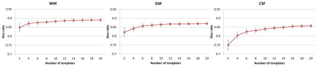
Dice ratio of segmentation vs. the number of templates. Experiment is performed by leave-one-out cross-validation with a patch size 5×5×5 and a size of neighborhood 5×5×5, which were optimized by Section 3.2.

3.4 Leave-one-out cross-validation

To evaluate the performance of the proposed method, we adopted the leave-one-out cross-validation. In each cross-validation step, 21 template images were used as priors and the remaining template image was used as testing subject to be segmented by the proposed method. The optimal parameters are set according to the parameter settings described in (Bach et al., 2012) for each cross-validation. Note that the ground-truth segmentation of test image is completely excluded from the segmentation library. This process was repeated until each image was taken as the testing image once.

Fig. 7 demonstrates the segmentation results of different methods for one typical subject. The original T1, T2 and FA images and the ground-truth segmentation are shown in the first row of Fig. 7. We first compare the proposed method with the coupled level sets (CLS) method (Wang et al., 2011), with the results shown in the second row. The CLS utilized T1, T2 and FA independently and estimated the tissue probabilities in a voxel-wise fashion, which ignores the joint power of multi-modality information and also the structural information in the neighborhood. We then make comparison with the majority voting (MV). Its performance is highly dependent on the accuracy of the registration, which is unfortunately difficult for the isointense infant images with the extremely low tissue contrast. In addition, MV uses all the warped atlases equally, which could also affect the segmentation results. We further make comparison with the conventional patch-based (CPB) method (Coupé et al., 2011). Note that, to make a fair comparison, we perform a similar cross-validation as in Section 3.2 to derive the optimal parameters for the CPB, and finally obtained the patch size of 5×5×5 and the neighborhood size of 5×5×5. The CPB utilizes nonlocal patch-based label fusion for segmentation of adult hippocampus and ventricle and has achieved promising results. However, since the CPB uses a simple intensity difference based similarity measure (Sum of the Squared Difference, SSD), this method is sensitive to the variance of tissue contrast in the MRI data (Wang et al., 2014). On the other hand, in the isointense infant images, due to the varied myelination processes in different brain regions, T1 and T2 images suffer from the large variance of WM intensities in the whole brain. Similarly, even FA provides a good WM/GM contrast, however, FA images are still suffering from the noise, inhomogeneity, and large variation of FA values in the same WM, e.g., having quite low FA values in the fiber crossing and/or branching regions (Alexander et al., 2001; Kumazawa et al., 2010). To better compare the results by different methods, the label differences compared with the ground-truth segmentation are also presented, which qualitatively demonstrates the advantage of the proposed method. We then quantitatively evaluate the performance of different methods by employing Dice ratios, as shown in Fig. 8. Dice ratios are 0.807±0.01 (WM) and 0.842±0.01 (GM) by the coupled level sets method (Wang et al., 2011), and are 0.858± 0.01 (WM) and 0.825±0.006 (GM) by the conventional patch-based (CPB) method (Coupé et al., 2011), respectively. Without the anatomical constraint, our method achieves the average Dice ratios as 0.872±0.008 (WM) and 0.860±0.006 (GM). With the anatomical constraint, the proposed method achieves the highest Dice ratios as 0.889±0.008 (WM) and 0.870±0.006 (GM), respectively. Besides the Dice ratios, we also use average surface distance error for gauging segmentation error. The average surface distance errors from the generated WM/GM (GM/CSF) surfaces and the ground-truth surfaces are plotted in Fig. 9, which further demonstrates the accuracy of the proposed method. It is worth noting that any combination of these different modalities generally produce more accurate results than any single modality in terms of both Dice ratios and surface distance errors, which proves that the multi-modality information is useful for guiding tissue segmentation (Anbeek et al., 2008; He and Parikh, 2013; Prastawa et al., 2005; Weisenfeld and Warfield, 2009).

Fig. 7.

Comparisons between the coupled level sets method (Wang et al., 2011), majority voting, conventional patch-based method (Coupé et al., 2011) on T1+T2+FA images and the proposed sparsity based method. In each label-difference map, the dark-red colors indicate false negatives and the dark-blue colors indicate false positives. The last two rows show the results by the proposed method without or with the anatomical constraint.

Fig. 8.

Average Dice ratios of different methods on 22 subjects: the coupled level sets method (Wang et al., 2011), majority voting, conventional patch-based method (Coupé et al., 2011), the proposed sparse method with different combination of 3 modalities, and the proposed sparse method without and with the anatomical constraint.

Fig. 9.

Average surface distances errors between the surfaces obtained by different methods and the ground-truth surfaces on 22 subjects.

3.5 Importance of the anatomical constraint

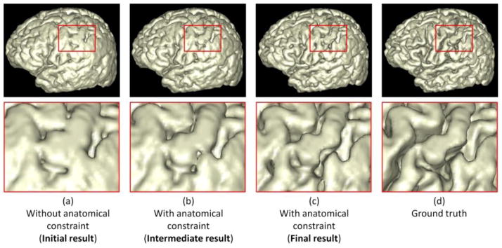
To further demonstrate the benefit of incorporating the anatomical constraint into the proposed method, we take the WM/GM surfaces as an example to visually compare the results by the proposed method without and with the anatomical constraint in Fig. 10. Fig. 10(a) shows the result without the anatomical constraint. It can be observed that there are many anatomical defects such as handle in the red rectangle, unsmooth boundary in the blue rectangle, and hole in the green rectangle. The intermediate and final results with the use of the anatomical constraint are also shown in Fig. 10(b) and (c). It can be observed the above-mentioned anatomical defects are gradually corrected. Fig. 11 shows the corresponding GM/CSF surface from the initialization to the final result. By referring to the ground-truth segmentation shown in Fig. 10(d) and Fig. 11(d), the result with the anatomical constraint is much more accurate and reasonable than the result without the anatomical constraint, which can also be demonstrated by the quantitative evaluation results with the Dice ratios and surface distance errors as shown in Fig. 8 and Fig. 9, respectively.

Fig. 10.

Comparisons of the proposed method without and with the anatomical constraint on the WM/GM surface. The zooming view of each rectangular region is also provided. From (a) to (c) shows the surface evolution from the initial stage to the final stage with the anatomical constraint. (d) is the ground truth.

Fig. 11.

Comparisons of the proposed method without and with the anatomical constraint on the GM/CSF surface. The zooming view of each rectangular region is also provided. From (a) to (c) shows the surface evolution from the initial stage to the final stage with the anatomical constraint. (d) is the ground truth.

3.6 Results on 10 additional subjects (with ground truth)

Besides using the leave-one-out cross-validation, we further validated our proposed method on 10 additional subjects, which were not included in the library. The manual segmentations by experts are again referred to as our ground truth. Here we randomly show the segmentation results on three subjects in Fig. 12. As can be observed, the results by the proposed method demonstrate better segmentation accuracy than those by the coupled level sets (CLS) method (Wang et al., 2011), majority voting and the conventional patch-based (CPB) method (Coupé et al., 2011), by referring to the original intensity images. The surface distance errors on a typical subject are shown in Fig. 13. The upper row of Fig. 13 shows the surface distances from the automatically surfaces obtained by different methods to the ground-truth surface. Since the surface distance measure is not symmetrical, the surface distances from the ground-truth surface to the automatically obtained surfaces are also shown in the lower row of the figure. It can be seen that our proposed method agrees most with the ground truth. The Dice ratios and average surface distance errors on 10 subjects by different methods are shown in the Fig. 14, which again demonstrates the advantage of our proposed method.

Fig. 12.

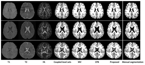
Results of 4 different methods, i.e., the coupled level sets method (Wang et al., 2011), majority voting, conventional patch-based method (Coupé et al., 2011), and the proposed method, on 3 subjects.

Fig. 13.

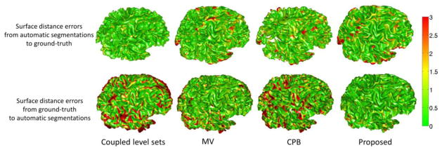
The upper row shows the surface distances in mm from the surfaces obtained by the CLS (Wang et al., 2011), majority voting, the conventional patch-based method (CPB) (Coupé et al., 2011), and our proposed method to the ground-truth surface. The lower row shows the ground-truth surface to the surfaces from 4 different methods. Color bar is shown in the right-most.

Fig. 14.

The Dice ratios and average surface distance errors by 4 different methods on 10 new testing subjects.

3.7 Computational time

We implemented the proposed method in MATLAB 7.12.0 using C/MEX code. The SPAMS toolbox (http://spams-devel.gforge.inria.fr) was used for the sparse coding. The average total computational time is around 2 hours for the segmentation of a subject using 3 modality images, each with the 256×256×198 voxel size and a spatial resolution of 1×1×1 mm³ (after alignment) on our Linux server with 8 CPUs and 16G memory.

4 Discussion and conclusion

In this paper, we have proposed a novel patch-based method for isointense infant brain MR image segmentation by utilizing the sparse multi-modality information. The segmentation is initially obtained based on the intensity patch similarity and then further iteratively refined with the anatomical constraint. The proposed method has been extensively evaluated on 22 training infant subjects using leave-one-out cross-validation, and also on 10 additional testing subjects, showing promising results compared with the state-of-the-art methods. It is worth noting that our framework can also be directly applied to the segmentation of images in infantile and adult-like stages, as shown in Fig. 15. Fig. 15(a) and (b) show exampler images in infantile stage and adult-like stage, respectively. With T2 or T1 -weighted image as an input, the proposed method has already produced reasonable segmentation results. If multi-modality images are available, it is expected to obtain more accurate results and will result in more accurate measurements of brain development (Nie et al., 2012; Zhang et al., 2011a).

Fig. 15.

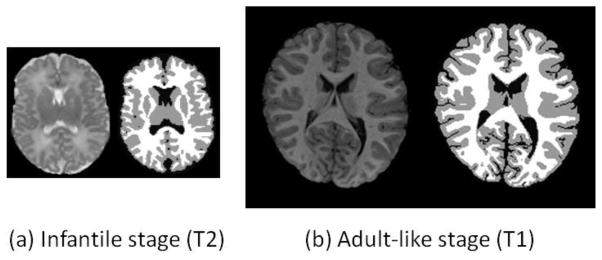
Results on images acquired in infantile stage (a) and adult-like stage (b).

In this paper, we have compared the proposed method with the coupled level sets (CLS) method (Wang et al., 2011), the conventional patch-based (CPB) method(Coupé et al., 2011), and majority voting. The proposed method achieves best accuracy compared with all other methods. The success of our method is mainly from the following aspects. First, our method works on image patches from T1, T2 and FA jointly, which can capture more information than using single-voxel information as in the CLS (Wang et al., 2011). Second, all the patches are normalized to have the unit ℓ2-norm to alleviate the intensity scale problem (Cheng et al., 2009; Wright et al., 2010). Third, the testing patch is well represented by the over-complete patch dictionary, with sparse constraint. The derived sparse coefficients are then directly utilized to (1) measure the patch similarity, instead of using the patch intensity difference as used in the CPB (Coupé et al., 2011), (2) estimate a subject-specific atlas, instead of a population-based atlas as used in CLS (Wang et al., 2011), (3) measure the contribution of each atlas in a spatially varying fashion, instead of equally weighting in the MV.

Current infant segmentation methods using T1/T2 MRI will generally over-estimate the GM in their segmentations, because the parts of WM near to the GM are mostly unmyelinated and thus can be easily mis-segmented into GM. In this work, we remedy this problem by employing FA to alleviate the over-estimation problem. Specially, FA images provide rich information of major fiber bundles, especially for the cortical regions where GM and WM are hardly distinguishable in the T1/T2 images. We have employed the method proposed in (Li et al., 2012) to calculate the cortical thickness. We find that the average cortical thickness is 2.46±0.06mm by the manual segmentations and 2.51±0.06mm by the proposed method. The difference is statistically non-significant (p-value > 0.09).

In our previous work (Wang et al., 2012b), we proposed a 4D multi-modality method to segment isointense images by utilizing the additional knowledge from images of both infantile and early adult-like stages. The Dice ratios for WM and GM on isointense infant images were 0.92±0.015 and 0.92±0.01, respectively. However, this method requires the availability of longitudinal scans, which limits its usage. Given that most infant subjects do not have longitudinal scans, the proposed method is standalone and also presents reasonable results with Dice ratios as 0.889±0.008 (WM) and 0.870±0.006 (GM). In our recent work (Wang et al., 2014; Wang et al., 2013b), we proposed a patch-driven level sets method for segmentation of neonatal brain images by taking advantage of sparse representation techniques. The main differences between our proposed method and this previous method can be summarized as follows. (1) The previous work focuses only on the segmentation of the neonatal brain images (≤ 1 month), while our proposed method focuses on the segmentation of isointense infant images, which is much more difficult due to its extremely low tissue contrast. (2) Only a single T2 modality was utilized in the previous work, while multi-modality T1, T2 and FA images are employed here for more accurate segmentation. (3) The segmentations by the previous work without considering the anatomical constraint suffer from anatomical errors, which are largely corrected by our proposed method. Our strategy is simple and effective by iteratively comparing the tentatively segmented image with the ground-truth segmentation images in the library. Although the proposed method cannot guarantee the topological correctness of the final WM/GM (GM/CSF) surface, the topological errors are largely reduced as reflected by experimental results.

Although our proposed method can produce more accurate results on the isointense infant images, it still has some limitations. (1) Our proposed method requires a number of templates, along with their corresponding manual segmentation results. However, it is not a trivial work to achieve manual segmentations. In this paper, manual segmentations were performed based upon the automatic segmentations by the iBEAT (Dai et al., 2013) (http://www.nitrc.org/projects/ibeat/), and thus the ground truth could be systematically biased by the iBEAT results. (2) In our proposed method, the contributions of different modalities are equal. In the future, we will further investigate how to determine different weights to different modalities in different brain regions. (3) Our current library consists of only healthy subjects, which may limit the performance of our method on the pathological subjects. This particular limitation could be partially overcome by employing more other information such as mean diffusivity. All the above-mentioned limitations will be investigated in our future work.

In our method, we nonlinearly aligned all the template images onto the space of the testing image using Diffeomorphic Demons (Vercauteren et al., 2009), based on T1 images. In fact, there are many registration methods (Jia et al., 2010; Shen et al., 1999; Tang et al., 2009; Wu et al., 2013; Wu et al., 2006; Xue et al., 2006a; Xue et al., 2006b; Yang et al., 2008; Zacharaki et al., 2008) we can employ. In our future work, we will also investigate the effect of different registration methods.

Research highlight.

• Multi-modality (T1, T2, FA) sparse representation is proposed.

• Anatomical constraint is further incorporated into the sparse representation.

• The proposed method is successfully applied to the isointense infant MR images.

• The proposed method can also work on the neonatal and adult-like images.

• The proposed method has been extensively evaluated on 32 subjects.

References

- Alexander AL, Hasan KM, Lazar M, Tsuruda JS, Parker DL. Analysis of partial volume effects in diffusion-tensor MRI. Magnetic Resonance in Medicine. 2001;45:770–780. doi: 10.1002/mrm.1105. [DOI] [PubMed] [Google Scholar]
- Anbeek P, Vincken K, Groenendaal F, Koeman A, VAN Osch M, VAN DER Grond J. Probabilistic Brain Tissue Segmentation in Neonatal Magnetic Resonance Imaging. Pediatr Res. 2008;63:158–163. doi: 10.1203/PDR.0b013e31815ed071. [DOI] [PubMed] [Google Scholar]
- Asman AJ, Landman BA. Non-local statistical label fusion for multi-atlas segmentation. Medical Image Analysis. 2013;17:194–208. doi: 10.1016/j.media.2012.10.002. [DOI] [PMC free article] [PubMed] [Google Scholar]
- Bach F, Mairal J, Ponce J. Task-Driven Dictionary Learning. IEEE Transactions on Pattern Analysis and Machine Intelligence. 2012;34:791–804. doi: 10.1109/TPAMI.2011.156. [DOI] [PubMed] [Google Scholar]
- Bai W, Shi W, ORD P, Tong T, Wang H, Jamil-Copley S, Peters NS, Rueckert D. A Probabilistic Patch-Based Label Fusion Model for Multi-Atlas Segmentation With Registration Refinement: Application to Cardiac MR Images. Medical Imaging, IEEE Transactions on. 2013;32:1302–1315. doi: 10.1109/TMI.2013.2256922. [DOI] [PubMed] [Google Scholar]
- Bazin P-l, Pham DL. Topology preserving tissue classification with fast marching and topology templates. IPMI. 2005:234–245. doi: 10.1007/11505730_20. [DOI] [PubMed] [Google Scholar]
- Buades A, Coll B, Morel JM. A non-local algorithm for image denoising. Computer Vision and Pattern Recognition, 2005. CVPR 2005. IEEE Computer Society Conference on; 2005. pp. 60–65. [Google Scholar]
- Cardoso MJ, Melbourne A, Kendall GS, Modat M, Robertson NJ, Marlow N, Ourselin S. AdaPT: An adaptive preterm segmentation algorithm for neonatal brain MRI. Neuro Image. 2013;65:97–108. doi: 10.1016/j.neuroimage.2012.08.009. [DOI] [PubMed] [Google Scholar]
- Cheng H, Liu Z, Yang L. Sparsity induced similarity measure for label propagation. Computer Vision, 2009 IEEE 12th International Conference on; 2009. pp. 317–324. [Google Scholar]
- Coupé P, Eskildsen SF, Manjón JV, Fonov V, Collins DL. Simultaneous segmentation and grading of anatomical structures for patient’s classification: Application to Alzheimer’s disease. Neuro Image. 2012a;59:3736–3747. doi: 10.1016/j.neuroimage.2011.10.080. [DOI] [PubMed] [Google Scholar]
- Coupé P, Eskildsen SF, Manjón JV, Fonov VS, Pruessner JC, Allard M, Collins DL. Scoring by nonlocal image patch estimator for early detection of Alzheimer’s disease. Neuro Image: Clinical. 2012b;1:141–152. doi: 10.1016/j.nicl.2012.10.002. [DOI] [PMC free article] [PubMed] [Google Scholar]
- Coupé P, Manjón J, Fonov V, Pruessner J, Robles M, Collins DL. Patch-based segmentation using expert priors: Application to hippocampus and ventricle segmentation. Neuro Image. 2011;54:940–954. doi: 10.1016/j.neuroimage.2010.09.018. [DOI] [PubMed] [Google Scholar]
- Dai Y, Shi F, Wang L, Wu G, Shen D. iBEAT: A Toolbox for Infant Brain Magnetic Resonance Image Processing. Neuroinformatics. 2013;11:211–225. doi: 10.1007/s12021-012-9164-z. [DOI] [PubMed] [Google Scholar]
- Efron B, Hastie T, Johnstone I, Tibshirani R. Least angle regression. Annals of Statistics. 2004;32:407–499. [Google Scholar]
- Elad M, Aharon M. Image Denoising Via Sparse and Redundant Representations Over Learned Dictionaries. Image Processing, IEEE Transactions on. 2006;15:3736–3745. doi: 10.1109/tip.2006.881969. [DOI] [PubMed] [Google Scholar]
- Eskildsen SF, Coupé P, Fonov V, Manjón JV, Leung KK, Guizard N, Wassef SN, Østergaard LR, Collins DL. BEaST: Brain extraction based on nonlocal segmentation technique. Neuro Image. 2012;59:2362–2373. doi: 10.1016/j.neuroimage.2011.09.012. [DOI] [PubMed] [Google Scholar]
- Fadili MJ, Starck JL, Murtagh F. Inpainting and Zooming Using Sparse Representations. The Computer Journal. 2009;52:64–79. [Google Scholar]
- Fan Y, Shi F, Smith JK, Lin W, Gilmore JH, Shen D. Brain anatomical networks in early human brain development. Neuro Image. 2011;54:1862–1871. doi: 10.1016/j.neuroimage.2010.07.025. [DOI] [PMC free article] [PubMed] [Google Scholar]
- Fischl B, Liu A, Dale AM. Automated manifold surgery: constructing geometrically accurate and topologically correct models of the human cerebral cortex. Medical Imaging, IEEE Transactions on. 2001;20:70–80. doi: 10.1109/42.906426. [DOI] [PubMed] [Google Scholar]
- Gao Y, Liao S, Shen D. Prostate segmentation by sparse representation based classification. Medical Physics. 2012;39:6372–6387. doi: 10.1118/1.4754304. [DOI] [PMC free article] [PubMed] [Google Scholar]
- Gui L, Lisowski R, Faundez T, Hüppi PS, Lazeyras Fo, Kocher M. Morphology-driven automatic segmentation of MR images of the neonatal brain. Med Image Anal. 2012;16:1565–1579. doi: 10.1016/j.media.2012.07.006. [DOI] [PubMed] [Google Scholar]
- Han X, Pham DL, Tosun D, Rettmann ME, Xu C, Prince JL. CRUISE: Cortical reconstruction using implicit surface evolution. Neuro Image. 2004;23:997–1012. doi: 10.1016/j.neuroimage.2004.06.043. [DOI] [PubMed] [Google Scholar]
- He L, Parikh NA. Automated detection of white matter signal abnormality using T2 relaxometry: Application to brain segmentation on term MRI in very preterm infants. Neuro Image. 2013;64:328–340. doi: 10.1016/j.neuroimage.2012.08.081. [DOI] [PMC free article] [PubMed] [Google Scholar]
- Jia H, Wu G, Wang Q, Shen D. ABSORB: Atlas building by self-organized registration and bundling. Neuro Image. 2010;51:1057–1070. doi: 10.1016/j.neuroimage.2010.03.010. [DOI] [PMC free article] [PubMed] [Google Scholar]
- Kim SH, Fonov VS, Dietrich C, Vachet C, Hazlett HC, Smith RG, Graves MM, Piven J, Gilmore JH, Dager SR, McKinstry RC, Paterson S, Evans AC, Collins DL, Gerig G, Styner MA. Adaptive prior probability and spatial temporal intensity change estimation for segmentation of the one-year-old human brain. Journal of Neuroscience Methods. 2013;212:43–55. doi: 10.1016/j.jneumeth.2012.09.018. [DOI] [PMC free article] [PubMed] [Google Scholar]
- Kuklisova-Murgasova M, Aljabar P, Srinivasan L, Counsell SJ, Doria V, Serag A, Gousias IS, Boardman JP, Rutherford MA, Edwards AD, Hajnal JV, Rueckert D. A dynamic 4D probabilistic atlas of the developing brain. Neuro Image. 2011;54:2750–2763. doi: 10.1016/j.neuroimage.2010.10.019. [DOI] [PubMed] [Google Scholar]
- Kumazawa S, Yoshiura T, Honda H, Toyofuku F, Higashida Y. Partial volume estimation and segmentation of brain tissue based on diffusion tensor MRI. Medical Physics. 2010;37:1482–1490. doi: 10.1118/1.3355886. [DOI] [PubMed] [Google Scholar]
- Langerak TR, van der Heide UA, Kotte ANTJ, Viergever MA, van Vulpen M, Pluim JPW. Label Fusion in Atlas-Based Segmentation Using a Selective and Iterative Method for Performance Level Estimation (SIMPLE) Medical Imaging, IEEE Transactions on. 2010;29:2000–2008. doi: 10.1109/TMI.2010.2057442. [DOI] [PubMed] [Google Scholar]
- Leroy F, Mangin J, Rousseau F, Glasel H, Hertz-Pannier L, Dubois J, Dehaene-Lambertz G. Atlas-free surface reconstruction of the cortical grey-white interface in infants. PLoS One. 2011;6:e27128. doi: 10.1371/journal.pone.0027128. [DOI] [PMC free article] [PubMed] [Google Scholar]
- Li G, Nie J, Wang L, Shi F, Lin W, Gilmore JH, Shen D. Mapping Region-Specific Longitudinal Cortical Surface Expansion from Birth to 2 Years of Age. Cerebral Cortex. 2013a;23:2724–2733. doi: 10.1093/cercor/bhs265. [DOI] [PMC free article] [PubMed] [Google Scholar]
- Li G, Nie J, Wang L, Shi F, Lyall AE, Lin W, Gilmore JH, Shen D. Mapping Longitudinal Hemispheric Structural Asymmetries of the Human Cerebral Cortex From Birth to 2 Years of Age. Cerebral Cortex. 2013b doi: 10.1093/cercor/bhs413. [DOI] [PMC free article] [PubMed] [Google Scholar]
- Li G, Nie J, Wu G, Wang Y, Shen D. Consistent reconstruction of cortical surfaces from longitudinal brain MR images. Neuro Image. 2012;59:3805–3820. doi: 10.1016/j.neuroimage.2011.11.012. [DOI] [PMC free article] [PubMed] [Google Scholar]
- Li G, Wang L, Shi F, Lin W, Shen D. Multi-atlas Based Simultaneous Labeling of Longitudinal Dynamic Cortical Surfaces in Infants. In: Mori K, Sakuma I, Sato Y, Barillot C, Navab N, editors. Medical Image Computing and Computer-Assisted Intervention – MICCAI 2013. Springer; Berlin Heidelberg: 2013c. pp. 58–65. [DOI] [PMC free article] [PubMed] [Google Scholar]
- Liao S, Gao Y, Lian J, Shen D. Sparse Patch-Based Label Propagation for Accurate Prostate Localization in CT Images. Medical Imaging, IEEE Transactions on. 2013;32:419–434. doi: 10.1109/TMI.2012.2230018. [DOI] [PMC free article] [PubMed] [Google Scholar]
- Liu T, Li H, Wong K, Tarokh A, Guo L, Wong STC. Brain tissue segmentation based on DTI data. Neuro Image. 2007;38:114–123. doi: 10.1016/j.neuroimage.2007.07.002. [DOI] [PMC free article] [PubMed] [Google Scholar]
- Mairal J, Bach F, Ponce J, Sapiro G, Zisserman A. Discriminative learned dictionaries for local image analysis. Computer Vision and Pattern Recognition, 2008. CVPR 2008. IEEE Conference on; 2008a. pp. 1–8. [Google Scholar]
- Mairal J, Elad M, Sapiro G. Sparse Representation for Color Image Restoration. Image Processing, IEEE Transactions on. 2008b;17:53–69. doi: 10.1109/tip.2007.911828. [DOI] [PubMed] [Google Scholar]
- Nie J, Li G, Wang L, Gilmore JH, Lin W, Shen D. A Computational Growth Model for Measuring Dynamic Cortical Development in the First Year of Life. Cerebral Cortex. 2012;22:2272–2284. doi: 10.1093/cercor/bhr293. [DOI] [PMC free article] [PubMed] [Google Scholar]
- Nishida M, Makris N, Kennedy DN, Vangel M, Fischl B, Krishnamoorthy KS, Caviness VS, Grant PE. Detailed semiautomated MRI based morphometry of the neonatal brain: Preliminary results. Neuro Image. 2006;32:1041–1049. doi: 10.1016/j.neuroimage.2006.05.020. [DOI] [PubMed] [Google Scholar]
- Paus T, Collins DL, Evans AC, Leonard G, Pike B, Zijdenbos A. Maturation of white matter in the human brain: a review of magnetic resonance studies. Brain Research Bulletin. 2001;54:255–266. doi: 10.1016/s0361-9230(00)00434-2. [DOI] [PubMed] [Google Scholar]
- Prastawa M, Gilmore JH, Lin W, Gerig G. Automatic segmentation of MR images of the developing newborn brain. Med Image Anal. 2005;9:457–466. doi: 10.1016/j.media.2005.05.007. [DOI] [PubMed] [Google Scholar]
- Rousseau F, Habas PA, Studholme C. A Supervised Patch-Based Approach for Human Brain Labeling. TMI. 2011;30:1852–1862. doi: 10.1109/TMI.2011.2156806. [DOI] [PMC free article] [PubMed] [Google Scholar]
- Sabuncu MR, Yeo BTT, Van Leemput K, Fischl B, Golland P. A Generative Model for Image Segmentation Based on Label Fusion. Medical Imaging, IEEE Transactions on. 2010;29:1714–1729. doi: 10.1109/TMI.2010.2050897. [DOI] [PMC free article] [PubMed] [Google Scholar]
- Segonne F, Pacheco J, Fischl B. Geometrically Accurate Topology-Correction of Cortical Surfaces Using Nonseparating Loops. IEEE Trans Med Imaging. 2007;26:518–529. doi: 10.1109/TMI.2006.887364. [DOI] [PubMed] [Google Scholar]
- Shattuck DW, Leahy RM. Automated graph-based analysis and correction of cortical volume topology. Medical Imaging, IEEE Transactions on. 2001;20:1167–1177. doi: 10.1109/42.963819. [DOI] [PubMed] [Google Scholar]
- Shen D, Wong W-h, HSIpH Affine-invariant image retrieval by correspondence matching of shapes. Image and Vision Computing. 1999;17:489–499. [Google Scholar]
- Shi F, Fan Y, Tang S, Gilmore JH, Lin W, Shen D. Neonatal Brain Image Segmentation in Longitudinal MRI Studies. Neuro Image. 2010a;49:391–400. doi: 10.1016/j.neuroimage.2009.07.066. [DOI] [PMC free article] [PubMed] [Google Scholar]
- Shi F, Shen D, Yap P, Fan Y, Cheng J, An H, Wald LL, Gerig G, Gilmore JH, Lin W. CENTS: Cortical enhanced neonatal tissue segmentation. Hum Brain Mapp. 2011a;32:382–396. doi: 10.1002/hbm.21023. [DOI] [PMC free article] [PubMed] [Google Scholar]
- Shi F, Wang L, Dai Y, Gilmore JH, Lin W, Shen D. Pediatric Brain Extraction Using Learning-based Meta-algorithm. Neuro Image. 2012;62:1975–1986. doi: 10.1016/j.neuroimage.2012.05.042. [DOI] [PMC free article] [PubMed] [Google Scholar]
- Shi F, Yap PT, Fan Y, Gilmore JH, Lin W, Shen D. Construction of multi-region-multi-reference atlases for neonatal brain MRI segmentation. Neuro Image. 2010b;51:684–693. doi: 10.1016/j.neuroimage.2010.02.025. [DOI] [PMC free article] [PubMed] [Google Scholar]
- Shi F, Yap P-T, Gilmore JH, Lin W, Shen D. Spatial-temporal constraint for segmentation of serial infant brain MR images. MIAR 2010c [Google Scholar]
- Shi F, Yap PT, Wu G, Jia H, Gilmore JH, Lin W, Shen D. Infant Brain Atlases from Neonates to 1- and 2-Year-Olds. PLoS ONE. 2011b;6:e18746. doi: 10.1371/journal.pone.0018746. [DOI] [PMC free article] [PubMed] [Google Scholar]
- Sled JG, Zijdenbos AP, Evans AC. A nonparametric method for automatic correction of intensity nonuniformity in MRI data. IEEE Trans Med Imaging. 1998;17:87–97. doi: 10.1109/42.668698. [DOI] [PubMed] [Google Scholar]
- Song Z, Awate SP, Licht DJ, Gee JC. Clinical neonatal brain MRI segmentation using adaptive nonparametric data models and intensity-based Markov priors. Med Image Comput Comput Assist Interv Int Conf Med Image Comput Comput Assist Interv. 2007:883–890. doi: 10.1007/978-3-540-75757-3_107. [DOI] [PubMed] [Google Scholar]
- Tang S, Fan Y, Wu G, Kim M, Shen D. RABBIT: Rapid alignment of brains by building intermediate templates. Neuro Image. 2009;47:1277–1287. doi: 10.1016/j.neuroimage.2009.02.043. [DOI] [PMC free article] [PubMed] [Google Scholar]
- Tibshirani RJ. Regression Shrinkage and Selection via the Lasso. Journal of the Royal Statistical Society, Series B. 1996;58:267–288. [Google Scholar]
- Tong T, Wolz R, Coupé P, Hajnal JV, Rueckert D. Segmentation of MR images via discriminative dictionary learning and sparse coding: Application to hippocampus labeling. Neuro Image. 2013;76:11–23. doi: 10.1016/j.neuroimage.2013.02.069. [DOI] [PubMed] [Google Scholar]
- Tong T, Wolz R, Hajnal JV, Rueckert D. Segmentation of brain MR images via sparse patch representation. MICCAI Workshop on Sparsity Techniques in Medical Imaging (STMI) 2012 [Google Scholar]
- Vercauteren T, Pennec X, Perchant A, Ayache N. Diffeomorphic demons: Efficient non-parametric image registration. Neuro Image. 2009;45:S61–S72. doi: 10.1016/j.neuroimage.2008.10.040. [DOI] [PubMed] [Google Scholar]
- Wang H, Suh JW, Das SR, Pluta J, Craige C, Yushkevich PA. Multi-Atlas Segmentation with Joint Label Fusion. IEEE Trans on PAMI 2012a [Google Scholar]
- Wang J, Yang J, Yu K, Lv F, Huang TS, Gong Y. Locality-constrained Linear Coding for image classification. CVPR. 2010:3360–3367. [Google Scholar]
- Wang L, Shi F, Li G, Gao Y, Lin W, Gilmore JH, Shen D. Segmentation of neonatal brain MR images using patch-driven level sets. Neuro Image. 2014;84:141–158. doi: 10.1016/j.neuroimage.2013.08.008. [DOI] [PMC free article] [PubMed] [Google Scholar]
- Wang L, Shi F, Li G, Lin W, Gilmore J, Shen D. Integration of Sparse Multi-modality Representation and Geometrical Constraint for Isointense Infant Brain Segmentation. In: Mori K, Sakuma I, Sato Y, Barillot C, Navab N, editors. Medical Image Computing and Computer-Assisted Intervention – MICCAI 2013. Springer; Berlin Heidelberg: 2013a. pp. 703–710. [DOI] [PMC free article] [PubMed] [Google Scholar]
- Wang L, Shi F, Li G, Lin W, Gilmore JH, Shen D. Patch-driven neonatal brain MRI segmentation with sparse representation and level sets. Biomedical Imaging (ISBI), 2013 IEEE 10th International Symposium on; 2013b. pp. 1090–1093. [Google Scholar]
- Wang L, Shi F, Lin W, Gilmore JH, Shen D. Automatic segmentation of neonatal images using convex optimization and coupled level sets. Neuro Image. 2011;58:805–817. doi: 10.1016/j.neuroimage.2011.06.064. [DOI] [PMC free article] [PubMed] [Google Scholar]
- Wang L, Shi F, Yap PT, Gilmore JH, Lin W, Shen D. 4D Multi-Modality Tissue Segmentation of Serial Infant Images. PLoS One. 2012b;7:e44596. doi: 10.1371/journal.pone.0044596. [DOI] [PMC free article] [PubMed] [Google Scholar]
- Wang L, Shi F, Yap P, Lin W, Gilmore JH, Shen D. Longitudinally guided level sets for consistent tissue segmentation of neonates. Hum Brain Mapp. 2013c;34:956–972. doi: 10.1002/hbm.21486. [DOI] [PMC free article] [PubMed] [Google Scholar]
- Warfield SK, Zou KH, Wells WM. Simultaneous truth and performance level estimation (STAPLE): an algorithm for the validation of image segmentation. Medical Imaging, IEEE Transactions on. 2004;23:903–921. doi: 10.1109/TMI.2004.828354. [DOI] [PMC free article] [PubMed] [Google Scholar]
- Weisenfeld NI, Mewes AUJ, Warfield SK. Highly accurate segmentation of brain tissue and subcortical gray matter from newborn MRI. Proceedings of the 9th international conference on Medical Image Computing and Computer-Assisted Intervention - Volume Part I; Copenhagen, Denmark: Springer-Verlag; 2006a. pp. 199–206. [DOI] [PubMed] [Google Scholar]
- Weisenfeld NI, Mewes AUJ, Warfield SK. Segmentation of newborn brain MRI. ISBI. 2006b:766–769. [Google Scholar]
- Weisenfeld NI, Warfield SK. Automatic segmentation of newborn brain MRI. Neuro Image. 2009;47:564–572. doi: 10.1016/j.neuroimage.2009.04.068. [DOI] [PMC free article] [PubMed] [Google Scholar]
- Winn J, Criminisi A, Minka T. Object categorization by learned universal visual dictionary. Tenth IEEE International Conference on Computer Vision; 2005. pp. 1800–1807. [Google Scholar]
- Wright J, Yang AY, Ganesh A, Sastry SS, Ma Y. Robust Face Recognition via Sparse Representation. IEEE Trans Pattern Anal Mach Intell. 2009;31:210–227. doi: 10.1109/TPAMI.2008.79. [DOI] [PubMed] [Google Scholar]
- Wright J, Yi M, Mairal J, Sapiro G, Huang TS, Shuicheng Y. Sparse Representation for Computer Vision and Pattern Recognition. Proceedings of the IEEE. 2010;98:1031–1044. [Google Scholar]
- Wu G, Kim M, Wang Q, Gao Y, Liao S, Shen D. Unsupervised Deep Feature Learning for Deformable Registration of MR Brain Images. In: Mori K, Sakuma I, Sato Y, Barillot C, Navab N, editors. Medical Image Computing and Computer-Assisted Intervention – MICCAI 2013. Springer; Berlin Heidelberg: 2013. pp. 649–656. [DOI] [PMC free article] [PubMed] [Google Scholar]
- Wu G, Qi F, Shen D. Learning-Based Deformable Registration of MR Brain Images. IEEE Transactions on Medical Imaging. 2006;25:1145–1157. doi: 10.1109/tmi.2006.879320. [DOI] [PubMed] [Google Scholar]
- Xue H, Srinivasan L, Jiang S, Rutherford M, Edwards AD, Rueckert D, Hajnal JV. Automatic segmentation and reconstruction of the cortex from neonatal MRI. Neuro Image. 2007;38:461–477. doi: 10.1016/j.neuroimage.2007.07.030. [DOI] [PubMed] [Google Scholar]
- Xue Z, Shen D, Davatzikos C. Statistical representation of high-dimensional deformation fields with application to statistically constrained 3D warping. Medical Image Analysis. 2006a;10:740–751. doi: 10.1016/j.media.2006.06.007. [DOI] [PubMed] [Google Scholar]
- Xue Z, Shen D, Karacali B, Stern J, Rottenberg D, Davatzikos C. Simulating deformations of MR brain images for validation of atlas-based segmentation and registration algorithms. Neuro Image. 2006b;33:855–866. doi: 10.1016/j.neuroimage.2006.08.007. [DOI] [PMC free article] [PubMed] [Google Scholar]
- Yang J, Shen D, Davatzikos C, Verma R. Diffusion Tensor Image Registration Using Tensor Geometry and Orientation Features. In: Metaxas D, Axel L, Fichtinger G, Székely G, editors. Medical Image Computing and Computer-Assisted Intervention – MICCAI 2008. Springer; Berlin Heidelberg: 2008. pp. 905–913. [DOI] [PubMed] [Google Scholar]
- Yang J, Wright J, Huang TS, Ma Y. Image Super-Resolution Via Sparse Representation. Image Processing, IEEE Transactions on. 2010;19:2861–2873. doi: 10.1109/TIP.2010.2050625. [DOI] [PubMed] [Google Scholar]
- Yang J, Yu K, Gong YTH. Linear spatial pyramid matching using sparse coding for image classification. CVPR. 2009:1794–1801. [Google Scholar]
- Yap PT, Fan Y, Chen Y, Gilmore JH, Lin W, Shen D. Development Trends of White Matter Connectivity in the First Years of Life. PLoS ONE. 2011;6:e24678. doi: 10.1371/journal.pone.0024678. [DOI] [PMC free article] [PubMed] [Google Scholar]
- Yotter RA, Dahnke R, Thompson PM, Gaser C. Topological correction of brain surface meshes using spherical harmonics. Human Brain Mapping. 2011;32:1109–1124. doi: 10.1002/hbm.21095. [DOI] [PMC free article] [PubMed] [Google Scholar]
- Yushkevich PA, Piven J, Hazlett HC, Smith RG, Ho S, Gee JC, Gerig G. User-guided 3D active contour segmentation of anatomical structures: Significantly improved efficiency and reliability. Neuro Image. 2006;31:1116–1128. doi: 10.1016/j.neuroimage.2006.01.015. [DOI] [PubMed] [Google Scholar]
- Zacharaki EI, Shen D, Lee S-k, Davatzikos C. ORBIT: A Multiresolution Framework for Deformable Registration of Brain Tumor Images. IEEE Transactions on Medical Imaging. 2008;27:1003–1017. doi: 10.1109/TMI.2008.916954. [DOI] [PMC free article] [PubMed] [Google Scholar]
- Zhang D, Wang Y, Zhou L, Yuan H, Shen D. Multimodal classification of Alzheimer’s disease and mild cognitive impairment. Neuro Image. 2011a;55:856–867. doi: 10.1016/j.neuroimage.2011.01.008. [DOI] [PMC free article] [PubMed] [Google Scholar]
- Zhang S, Zhan Y, Dewan M, Huang J, Metaxas DN, Zhou XS. Deformable segmentation via sparse shape representation. In: Fichtinger G, Martel A, Peters T, editors. MICCAI 2011. Springer; Berlin Heidelberg: 2011b. pp. 451–458. [DOI] [PubMed] [Google Scholar]
- Zilles K, Armstrong E, Schleicher A, Kretschmann HJ. The human pattern of gyrification in the cerebral cortex. Anat Embryol (Berl) 1988;179:173–179. doi: 10.1007/BF00304699. [DOI] [PubMed] [Google Scholar]
- Zou H, Hastie T. Regularization and variable selection via the Elastic Net. Journal of the Royal Statistical Society, Series B. 2005;67:301–320. [Google Scholar]