

Abstract
The ionic atmosphere around nucleic acids remains only partially understood at atomic-level detail. Ion counting (IC) experiments provide a quantitative measure of the ionic atmosphere around nucleic acids and, as such, are a natural route for testing quantitative theoretical approaches. In this article, we replicate IC experiments involving duplex DNA in NaCl(aq) using molecular dynamics (MD) simulation, the three-dimensional reference interaction site model (3D-RISM), and nonlinear Poisson-Boltzmann (NLPB) calculations and test against recent buffer-equilibration atomic emission spectroscopy measurements. Further, we outline the statistical mechanical basis for interpreting IC experiments and clarify the use of specific concentration scales. Near physiological concentrations, MD simulation and 3D-RISM estimates are close to experimental results, but at higher concentrations (>0.7 M), both methods underestimate the number of condensed cations and overestimate the number of excluded anions. The effect of DNA charge on ion and water atmosphere extends 20–25 Å from its surface, yielding layered density profiles. Overall, ion distributions from 3D-RISMs are relatively close to those from corresponding MD simulations, but with less Na+ binding in grooves and tighter binding to phosphates. NLPB calculations, on the other hand, systematically underestimate the number of condensed cations at almost all concentrations and yield nearly structureless ion distributions that are qualitatively distinct from those generated by both MD simulation and 3D-RISM. These results suggest that MD simulation and 3D-RISM may be further developed to provide quantitative insight into the characterization of the ion atmosphere around nucleic acids and their effect on structure and stability.
Introduction
The ionic atmosphere around nucleic acids has a major impact on the stability of secondary and tertiary structure, modulating the binding of charged drugs and proteins and condensation and packing in cells (1). Recently, several experimental methods have been developed to examine the nature of ion atmosphere around nucleic acids through ion-counting experiments that rely on anomalous small-angle x-ray scattering (2,3), buffer equilibration atomic emission spectroscopy (BE-AES) (4,5), and titration with fluorescent dyes (6). In previous decades, 23Na or 39Co NMR relaxation rates have also been employed (7,8). There is a long history of theoretical models that attempt to describe ion atmosphere around nucleic acids, but there are relatively few calculations using models with atomic detail, in large part because equilibration of the water and ion distributions around nucleic acids is very slow in molecular dynamics (MD) or Monte Carlo simulations (9,10) and has only recently become feasible.
It is generally accepted that the majority of ions surrounding a nucleic acid molecule stay within a few angstroms of its surface and are able to diffuse along it or to the bulk, whereas relatively few ions occupy specific binding sites (site-bound ions), although these are no less important. The former type of binding was designated by Manning as territorial, as opposed to atmospheric, binding, a characteristic of nonpolymeric solutions (11,12). Experiments have shown that counterions associate with nucleic acids at salt concentrations much smaller than physiological concentrations, a fact attributed to the polymeric nature of nucleic acids (13). Manning’s counterion condensation theory (11,12,14–16) posits that beyond a certain threshold in axial charge density, an excess of 0.7–0.8 monovalent cations are bound per phosphate unit. Further, it has been shown that this phenomenon is the result of the attempt of the ionic and solvent atmosphere to neutralize the nucleic acid through counterion condensation and coion depletion (13). Although counterion condensation is prominent at low bulk salt concentration, as the bulk salt concentration increases the contribution from anion depletion rises (17).
Theoretical approaches for studying nucleic-acid-ion interactions beyond Manning’s theory include MD simulations (9,10,18–32), nonlinear Poisson-Boltzmann (NLPB) (4,17,29,33–35) calculations, and integral equation theory (IET) (36–39). MD in conjunction with molecular mechanics force fields has the advantage of providing complete atomistic detail of ion and water distributions, including dynamical information, but at larger computational expense than similar calculations using NLPB or IET. NLPB calculations avoid these computational costs but considerably oversimplify the physics of hydration and neutralization and omit ion correlation. IET, and specifically the three-dimensional reference interaction site model (3D-RISM) (40–43), provides a third approach that makes use of explicit-solvent models and provides molecular, noncontinuum detail at intermediate computational cost. The 3D-RISM can be considered parameter-free, requiring only an approximate closure relation and the same molecular mechanics model used for MD simulations (44).
In this article, we examine both the macroscopic and microscopic pictures of how nucleic acids interact with their ionic atmosphere as generated by MD simulations, 3D-RISM, and conventional NLPB calculations. To assure a proper comparison between theory and experiment, we replicate ion-counting experiments carried out using buffer equilibration atomic emission spectroscopy (4). The primary observable that allows the connection between ion-counting experiments and theory is the number of excess ions per solute, or preferential interaction parameters (PIPs). Several approaches for computing PIPs have been used in the past and we also aim to clarify the proper use of concentration scales to be used for comparing theoretical results with experimental data. At the microscopic level, we show that structural details of density distributions of ions and water around DNA clearly distinguish between continuum and noncontinuum theories. At the macroscopic level, we reveal that MD and 3D-RISM estimates are close to experimental results near physiological concentrations, but that at concentrations >0.7 M, both methods underestimate the number of condensed cations and overestimate the number of excluded anions. NLPB calculations, on the other hand, systematically underestimate the number of condensed cations at almost all concentrations, and yield nearly structureless ion distributions that are qualitatively distinct from those generated by both MD simulations and 3D-RISM.
Ion-counting Experiments
Ion-counting experiments measure the number of excess ions () or PIPs around nucleic acid molecules. These quantities can be measured experimentally in a variety of ways, most simply by dialysis experiments that count the number of ions crossing a semipermeable membrane when a nucleic acid is added (4,45). Specifically, for DNA molecules immersed in an aqueous solution containing a single type of anion (−) and cation (+),
| (1) |
where M stands for the molarity of the corresponding species in the two chambers of the osmotic cell (46).
PIPs measure the preference of a solute (labeled 2) for water (labeled 1) or a cosolvent (labeled 3) (47,48). PIPs are fundamental in studying salt effects (7,49,50) and measure the integrated amount by which the local concentration of water or cosolvent around the solute differ from the corresponding values in the bulk. When computed for ionic species, PIPs are also called Donnan coefficients. In the case of this study, the cosolvent is represented by dissociated sodium chloride, although it can be any charged or neutral species in general. The definition of depends on the units of concentration used (47,48): for molality (m) or molarity (M) scales, is defined as
| (2) |
and
| (3) |
These definitions are valid in the limit of infinite dilution of the solute and are derived in the grand canonical ensemble resembling the experimental conditions of dialysis. This corresponds to equal chemical potentials of salt and water in the two chambers of the osmosis experiment. As discussed below, the molal and molar scales lead to different values of PIPs. From the specific case of the system considered here, index 2 corresponds to the DNA, index 1 to water, and index 3 to sodium chloride, NaCl. When the cosolvent is a monovalent salt and PIPs are determined separately for monocationic (+) and monoanionic (−) species, one can show that
| (4) |
and
| (5) |
where is the charge of the solute (7,49,50). Combining Eqs. 4 and 5 leads to , i.e., the preferential order parameter for the anion is equal to that of the salt. Thus, can be interpreted as the number of pairs of monovalent cations and anions depleted when titrating DNA in the salt solution.
Ion counting using Kirkwood-Buff integrals
Kirkwood-Buff (KB) integrals, , are central quantities in liquid state theory (51) and are defined as
| (6) |
where is the pair distribution function (PDF) at constant chemical potential, μ, volume, V, and temperature, T, with α and γ representing any two components of the solution. Following Smith (48), the PIPs in the grand canonical ensemble can be calculated for molal and molar concentration units using
| (7) |
and
| (8) |
It has been argued that can be estimated from MD simulation in isothermal-isobaric (NPT) or canonical (NVT) ensembles by integrating not to infinity but to a correlation radius, (52–55):
| (9) |
The , also called the radius of influence, delimits the space around the solute for which the solvent and cosolvent concentrations are different from those found in the bulk (53,55). The location and shape of the partition are arbitrary but should be large enough that the bulk region is not perturbed by the solute. The partition should be of fixed volume and shape. For well converged simulations, there is no need to estimate R, as one can carry out the integration up to the system boundary. For the case of the rigid B-DNA molecule considered here (48 nucleobases and a 46− charge), our calculations indicate that the correlation radius slightly decreases with increasing salt concentration and can be estimated to be 20–25 Å from the DNA helical axis. This means that to simulate the DNA in equilibrium with a bulk salt, one has to extend the simulation periodic box to accommodate the volume enclosed in the correlation radius plus an additional volume representing the bulk. The size of this additional volume has to be large enough to allow RDFs to properly converge (18) (see also Pollack (3)).
For 3D-RISM, to account for the long-range behavior of the ion distributions, a correction is applied using the long-range asymptotic solution to the total correlation function. The correction was originally proposed to overcome difficulties in performing the inverse fast Fourier transform when solving the RISM equation and captures the Debye-screened long-range distribution of the electrolyte (42,43).
Ion counting using the two-partition (domain) model
For methods that directly generate PDFs, such as 3D-RISM and NLPB theory, calculating PIPs with KB integrals is a natural approach. However, for MD simulations, calculating and storing 3D PDFs from a trajectory can be a computationally complex and memory-intensive procedure. One way to lessen the effort required is to use the two-partition approach, introduced first by Anderson and Record in a general context (46, 56).
Within the two-domain approach, the system of interest is partitioned into two regions (see Fig. 1): a local region (R1) surrounding the solute, for which the densities of solvent and cosolvent (ions) are different from those found in the bulk, and a bulk region (R2) for which the densities of solvent and salt are uniform. This resembles an osmotic cell that allows the free exchange of solvent and cosolvent between R1 and R2 but in which the solute is restricted to R1. It must be pointed out that during the MD simulations, the instantaneous total charge in the two partitions fluctuates, representing better the situation one would find in a grand canonical ensemble or an osmosis experiment. Since solvent and cosolvent are free to diffuse across the virtual membrane, we obtain the desired ensemble, similar to the KB approach (52–54).
Figure 1.
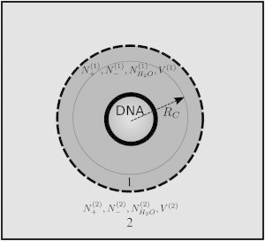
Ion counting using the two-domain approach (46), adapted from Anderson and Record (56). The simulated system is separated into two regions, dark gray (region 1) and light gray (region 2), with the boundary between the two regions shown as a dashed line. Region 1 has to be chosen so that it contains at least all the solvent and cosolvent within the correlation radius (see text) from the DNA, and region 2 so that it resembles the bulk with uniform concentration of salt. Using this approach, a formula for the PIPs can be derived that depends on the salt bulk (region 2) concentration. This method may be useful when the g(r) cannot be easily defined.
One can further adapt Eq. 1 for the case of an MD simulation. Taking into account that MD simulations are run with a constant number of particles and constant volume and contain a single DNA molecule, Eq. 1 becomes
| (10) |
| (11) |
Integrating over the volume of the simulation cell yields Eqs. 10 and 11 from Eqs. 7 and 8, respectively. It can be seen from Eqs. 10 and 11 that it is sufficient to estimate the average number density of water and NaCl in the bulklike region 2 after equilibration. The partition between the inner and bulk regions is chosen so that the inner region includes all the particles located within the correlation radius.
Both the KB integral method and the two-partition method depend on a good representation of the bulk region to estimate the ion and water concentrations. With that in mind, in this work, the DNA-water-ion system used in the MD simulations was extended at least 60 Å in the direction perpendicular to the DNA main axis. Pappu and Chen (18) have shown that there is a strong interdependence between the size of the simulation system and convergence of the distribution functions of charged species around nucleic acids.
Methods
MD simulations
Molecular mechanics force fields
The 24L B-DNA structure was prepared with Nucleic Acid Builder (NAB) (57) using the Arnott B-DNA fiber diffraction model (58). Three popular water models were used: TIP3P (59), TIP4P-Ew (60,61), and SPC/E (62). Only the SPC/E water model was used in 3D-RISM, with modified hydrogen Lennard-Jones parameters (44): and , where σ and E are the standard Lennard-Jones parameters and is the intramolecular oxygen-hydrogen bond distance. Hydrogen Lennard-Jones parameters are necessary to converge dielectrically consistent RISM (DRISM) equations, and these parameters have been shown to reproduce the solvent polarization free energy of explicit simulations for both polypeptides (44) and ions (63) in water. Ion parameters that were optimized to reproduce solvation energies and shown to prevent the salting-out effect were taken from Joung and Cheatham (64) and were not modified for RISM calculations. The all-atom ff10 force field for nucleic acids was used (65,66). We denote the three force fields as JC:TIP3P, JC:TIP4P-Ew, JC:SPC/E. (Since the DNA is harmonically restrained and the ff10 force field improves only some torsional terms of the ff99 force field (67), the results reported here should be the same when using either force field.). All topologies and structures were generated with the AMBER 10 package (68–70). The COULOMB constant used in NAMD 2.7 71 (332.0636) was changed to correspond to that used in the AMBER suite of programs (332.0522173) (68–70).
MD simulation protocol
Simulations were performed with the NAMD simulation package (version 2.7) (71). The DNA immersed in a preequilibrated water box with hexagonal prism symmetry (a = b 127.0 Å, c 152.0 Å, α = 90°, β = 90°, γ = 60°). The ionic atmosphere consisted of Na+ and Cl− ions that were added at random positions at least 5.0 Å away from any DNA atom to neutralize the system to reach a desired starting concentration of ∼0.2 and 0.7 M. The isothermal-isobaric (NPT) or isothermal (NVT) ensemble were used at 1 atm and 300 K using the Nosé-Hoover-Langevin piston (72,73) with a decay period of 100.0 fs and a damping timescale of 50 fs and the Langevin thermostat with a collision frequency of 0.1 ps−1. The smooth particle mesh Ewald method (74,75) was employed with a B-spline interpolation order of 6 and the default κ value used in NAMD. The fast Fourier transform grid points used for the lattice directions were chosen using 1.0 Å spacing. Nonbonded interactions were treated using an atom-based cutoff of 9.0 Å, with no switching for nonbond potentials. Numerical integration was performed using the leap-frog Verlet algorithm with a 2 fs time step (76). Covalent bond lengths involving water hydrogens were constrained using the SHAKE algorithm (77). All heavy atoms of the DNA were restrained to their initial positions with a harmonic potential using a 2.0 force constant. The systems were equilibrated for 35 ns in the NPT ensemble. The motions and relaxation of solvent and counter- and coions are notoriously slow to converge in nucleic acid simulations (10), and careful equilibration is critical, especially for low salt concentrations. Further details of the various simulations are given in Table S2 in the Supporting Material.
RISM
The 3D density distribution of aqueous salt solutions around a large macromolecule such as DNA can be directly computed for each atomic site of the solvent using the 3D-RISM (40–43). Like NLPB calculations, numerical solutions are iteratively solved on a 3D grid in the infinite-dilution regime, but unlike NLPB, 3D-RISM uses common molecular force fields to model both the solute and solvent and explicitly calculates an equilibrium density distribution of solvent around the solute.
The 3D-RISM is based on the Ornstein and Zernike IET (the OZ equation) (78,79), which expresses the density distribution in terms of direct and indirect correlation functionals. The OZ equation is inherently six-dimensional for polyatomic molecules due to orientational dependence on the intermolecular interactions. 3D-RISM formalism reduces this to three dimensions by orientational averaging of the solvent degrees of freedom such that the resulting solvent density distributions contain only a spatial dependence, . In this manner, the distributions of atomic sites on water and salt are represented on 3D grids via the total correlation function, , and the direct correlation function, , which are related as
| (12) |
is the site-site solvent susceptibility of solvent sites α and γ and contains the orientationally averaged bulk properties of the solvent. We use the DRISM integral equation (80,81) to precompute . In practice, the convolution integrals in Eq. 12 are performed in reciprocal space using a 3D fast Fourier transform,
| (13) |
an approach first developed for the OZ equation (82–84) and later applied to 1D-RISM (85) and 3D-RISM (43,86,87) that considers the long-range nature of electrostatic interactions between solvent and solute.
As in all OZ-based theories, a second, so-called closure equation must be used to obtain a unique solution. Due to the complexity of the closure equation, an approximation must be used. The form of this approximation has a major impact on the convergence of calculations, as well as on resulting thermodynamic quantities and densities. The general 3D-RISM closure relation has the form
where is the PDF and is the bridge function, which is only known as an infinite series of functionals and is always subject to some approximation (51). Many closure relations have been developed for IETs, of which the most popular are the hypernetted chain (HNC) (88) and partially linearized Kovalenko-Hirata (KH) (41) equations. In HNC 88, the bridge function is simply set to zero. HNC produces good results for ionic (38,81,89,90) and polar systems (91–93) and has an exact, closed-form expression for the excess chemical potential when coupled with RISM theory (94). However, HNC solutions are often difficult to converge. The KH closure (41) is numerically robust and addresses this problem by linearizing regions of density greater than bulk, . The partial series expansion of order-n (PSE-n) (95) generalizes the linearization to a Taylor series,
| (14) |
where β is the reciprocal thermodynamic temperature. For , the KH closure is recovered and HNC is the limiting case as . Like HNC, KH and PSE-n closures have an exact, closed-form expression for the chemical potential.
The number of terms used in the PSE-n closure does have an impact on the physical properties of the solvent, particularly for ions (63). For all calculations presented here, we used the highest order closure that could be converged with the cSPC/E model, PSE-4. For more discussion on the choice of closure and the impact on the calculated PIPs, see the Supporting Material.
DRISM
DRISM calculations were performed using the rism1d program in the AmberTools 12 molecular modeling package (44,96) and were performed largely according to the procedure of Joung et al. (63). To obtain of the bulk solvent, the DRISM equation coupled with the PSE-4 closure, was iteratively solved using the modified direct inversion of the iterative subspace (97) to a residual tolerance of at a temperature of 298.15 K and a dielectric constant of 78.44 for bulk water. A grid spacing of 0.025 Å was used throughout. To aid the convergence, solutions from lower-order closures, starting from KH, were iteratively used as initial guesses until the PSE-4 closure was converged. The water density for each salt concentration was interpolated from experimental measurements using cubic splines (63,98,99).
3D-RISM
3D-RISM calculations were performed using the rism3d.snglpnt program in the AmberTools 12 molecular modeling package (44,96). Equation 13, coupled with PSE-4 closures, was iteratively solved using the modified direct inversion of the iterative subspace to a residual tolerance of for all ion concentrations. Similar to the DRISM calculations, rapid convergence was achieved by first performing a few iterations with KH through PSE-3 closures to provide an initial guess for PSE-4. The extent of the solvation-box grid used was selected for each concentration to obtain a precision 0.002 excess ions together with a grid spacing of 0.5 Å. (for further information, see Table S2).
NLPB model
The NLPB method has been described in detail elsewhere (100,101). Briefly, NLPB has the form
| (15) |
where is an inhomogeneous dielectric medium of relative permittivity, is the charge distribution of the solute, is the bulk number density of the jth species of mobile ion in solution with charge , is the steric interaction between the mobile ion and the solute, and is the resulting electrostatic potential. can be numerically solved for on a 3D grid, which gives, for the PDF of ion species j, the expression
| (16) |
NLPB calculations were performed with Adaptive Poisson Boltzmann Solver (APBS) 1.4.1 (102). The grid size and spacing were adjusted to ensure that there were at least three digits of precision in all calculated values ( error). Where possible, a grid spacing of 1 Å was used, even when a 2 Å spacing gave the same result within the tolerable error. However, APBS is limited to total grid points, and we were required to use a 2 Å grid spacing for salt concentrations M. Testing showed that even at this larger spacing, the desired precision was achieved. Grid sizes used for all reported values are summarized in Table S3. The internal dielectric of the DNA was set to 1, and 78.54 was used for the solvent, where the standard molecular surface definition was used (srfm mol) with a solvent radius of 1.4 Å. Single Debye-Hückel boundary conditions (bcfl sdh) were used. Temperature was set to 298.15 K. Ion concentrations were identical to those used for DRISM and 3D-RISM.
For all calculations, an ion radius of 1.85 Å was used to define in Eq. 15. This radius was selected because a 1.85 Å ion with 1 e charge at infinite dilution in APBS, using a 66 Å 66 Å ×66 Å grid with 0.3333 Å grid spacing, has a solvation free energy of −90.2 kcal/mol, which is reasonably close to the values from experiment and the Joung-Cheatham parameters in explicit solvent. As we do not expect Cl− to make direct contact with the surface of the DNA, we are justified in using , which is standard behavior in APBS. All other parameters are the same as the DNA calculations, and grid size and spacing were varied to ensure at least three digits of precision in the calculated value (see Table S3 for further details).
Results and Discussion
Molecular distribution functions
Distribution functions are key to creating an average picture of how ions and water arrange around the DNA, as well as for extracting thermodynamic quantities such as PIPs that can be used to compare with ion-counting experiments. Here, we use three types of distribution function available from explicit-solvent MD simulations, 3D-RISM, and NLPB calculations, respectively, which we refer to as 3D, 2D, and 1D distributions. 3D and 1D distributions are commonly used to represent solvent and ion distributions around nucleic acids, and we describe them succinctly in the next paragraphs. Our approach to build 2D distributions is described in the next section.
3D distributions contain most of the information on how solvent and salt distribute around a rigid solute and are usually displayed using isosurfaces (see Fig. 2). 3D distributions are stored on 3D rectangular grids and are the main output from 3D-RISM and NLPB calculations.
Figure 2.
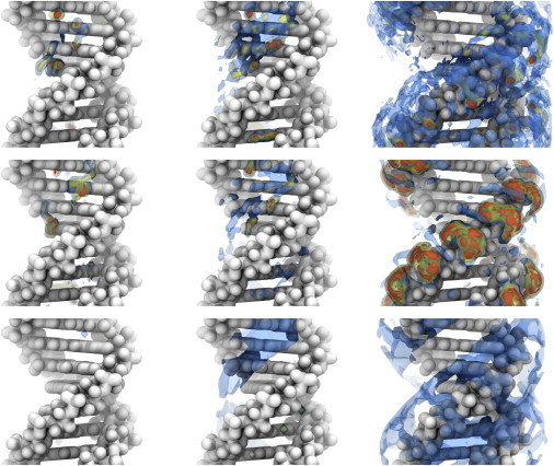
Cylindrical shells of sodium ion density around 24L DNA at 0.7452 M NaCl calculated by MD (upper row), 3D-RISM-PSE-4 (middle row), and NLPB (lower row). The shells isolate density extending radially from the DNA center of mass for 0–5 Å (left), 5–7.5 Å (center), and 7.5–15 Å (right) and correspond to regions identified in Figs. 3 and 5. Isosurfaces are at 4 (blue), 16 (yellow), and 64 times (orange) the bulk density. To see this figure in color, go online.
1D distribution functions (see Fig. 5) are based on the fact that the approximate cylindrical shape of the B-DNA molecule works well for representing the solvent and ion distributions in cylindrical coordinates with density averaged along z and θ, where the z axis coincides with the helical axis. We call these distribution functions cylindrical radial distribution functions (cRDFs). cRDFs are able to capture the layered distribution of ions with respect to the DNA main axis(see Fig. 5).
Figure 5.
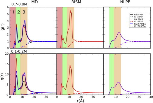
Na+ cylindrical RDFs obtained from explicit-solvent MD simulations (left), 3D-RISM (middle), and NLPB (right) at ∼0.2 M (upper) and ∼0.73 M (lower). A cylindrical subvolume ( and ) of the simulations was used to avoid end effects. Note that the normalization factor (salt bulk concentration) is slightly different (see Table S2) for each combination of water and ion models. To see this figure in color, go online.
In general, the overall shape of distributions does not change drastically with salt concentration, but the relative values of the density near the DNA with respect to bulk densities increase with decreasing concentration. Distributions obtained from 3D-RISM and MD simulations show a high degree of similarity, being highly structured, unlike those obtained from NLPB calculations.
2D untwisted densities
The density of ions and water in the average plane of a basepair can reveal useful information on the types of interactions in the major and minor grooves, as well as around the phosphates. This can be realized by analyzing the ion or water densities for each basepair plane, but as the number of basepairs increases, this becomes a complex task. Fig. 3 B shows a distribution in a plane perpendicular to the helical axis and averaged over the entire length of the DNA. Although one can roughly identify binding to the grooves and phosphates, the helical disposition of basepairs makes this type of representation hard to interpret. Here, we deconvolute this type of mapping through untwisting. First, we define a twisting rate as the ratio between the average helical twist and rise (Dz). Helical twist is defined as the angle between the C1′-C1′ vectors of adjacent basepairs. The rise is defined as the distance between the planes of adjacent basepairs. Second, each position that is mapped is transformed through a rotation around the helical axis (here chosen to be the z axis) that removes its corresponding twist:
where is the untwisted position vector, is the original position, and is a transformation matrix that corresponds to a rotation around the the helical axis, z. For the B-DNA structure studied in this work, the average twisting rate, , was calculated to be 0.18587 rad/Å. Untwisting is followed by averaging along a desired interval along the helical axis, z. An example of an untwisted Na+ density is shown in Fig. 3 C overlapped with the averaged untwisted positions of all heavy atoms of the DNA molecule. The effect of untwisting can be easily monitored using the C1′ atom positions in the basepair planes (Fig. 3 C, green dots). Before untwisting, the C1′ atoms are distributed along a circle, but afterward they are localized in two well defined points located at an approximate distance of 10 Å, which is typical for a Watson-Crick basepair. Although not explicitly shown, untwisting has a minimal effect on the other nucleobase atoms. Untwisting has a larger distortion effect on the DNA backbone.
Figure 3.
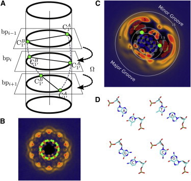
Construction of 2D untwisted density distributions. (A and B) Helical disposition of DNA basepairs (A) leads to a convoluted map of Na+ ions (B). (C) Removing the helical twist angle (i.e., untwisting) for each plane perpendicular to the main axis leads to a better resolved average distribution. Untwisting has a relatively minor effect on the relative distribution of atoms belonging to an average basepair, as shown by the dot clusters (red, oxygen; blue, nitrogen; gray, carbon; yellow, phosphorus). For example, although the C1′ atoms (green circles) are distributed nearly uniformly along a circle in the original mapping (B), untwisting leads to two localized positions (C). Numbered regions are discussed in text. (D) Orientation of typical basepairs. The ion densities shown here are derived from calculations using a bulk sodium chloride concentration of 0.17 M. The color scale for ion density can be found in Fig. 4.
Ion bridges in the major and minor grooves
MD simulations and 3D-RISM show that both water and cations penetrate into the minor and major grooves, forming well defined interaction patterns. With water treated implicitly, NLPB is able to place ions in the grooves, albeit in smaller amounts and with less structure. cRDFs obtained from MD simulations and 3D-RISM possess two peaks located in the minor and major grooves (see Fig. 5, red- and green-shaded areas, respectively). The peaks are located in the interval r < 5.0 Å and 5.0 < r <7.5 Å, respectively (see Fig. 2 for the 3D density and Fig. 5 for the corresponding cRDFs). Only the second peak is present in NLPB cylindrical distribution functions. Although 3D-RISM and MD simulations show very similar sodium binding patterns in the grooves, 3D-RISM underestimates the number of bound cations for the second peak and slightly overestimates the height of the first.
Untwisted densities can isolate the types of interactions that lead up to these 1D profiles. In Fig. 3, the circles that delimit the aforementioned two regions are overlaid on untwisted distributions, and one can easily identify the corresponding types of interactions. For both MD simulations and the RISM, the peak located at corresponds to sodium ions located in the major groove. These form ion bridges (30) through inner-sphere coordination of two G:O6 atoms belonging exclusively to 5′-GC-3′/3′-CG-5′ basepair steps. Sodium ions involved in such interaction are located in the region labeled 1 in Fig. 3. Ion-bridge binding patterns have been identified previously from MD simulations of DNA and RNA duplexes with K as counter- and coions and were found to be specific to (d,r)(5′-GC-3′/3′-CG-5′) and r(5′-AU-3′/3′-UA-5′) basepair steps (30,32).
The peak located between 5 Å and 7.5 Å corresponds to several types of interactions between sodium ions and the minor and major grooves. MD simulations and 3D-RISM show similar binding patterns, as can be seen in Figs. 2 and 4. On the major-groove side, sodium ions in region 2 in Fig. 3 C make inner-sphere coordination with G:N7 and A:N7 atoms. Region 4 includes sodium ions at solvent separation from DNA, making outer-sphere contacts with hydrogen-bond acceptors in the groove. A significant water density (twice the bulk density) is located approximately between regions 1 and 2 on one side and region 4 on the other. This indicates that water is able to mediate the outer-sphere interactions of sodium ions in region 4 and compete with sodium ions in region 1 or 2 by sharing their hydrogen atoms for hydrogen-bond formations. In the minor groove, sodium ions are located in region 3, and interactions are more spatially restricted than those in the major groove. The main interacting patterns correspond to chelating inner-sphere coordination between sodium ions and Ni:O4′ and C/Ti+1:O2. Water is able to compete for the same sites and adopts density values 1.5–2.0 times larger than those in the bulk. Water molecules that are part of the first two solvation layers of the minor groove of B-DNA are usually associated with the term spine of hydration or hydration ribbon(s) and have been the focus of intensive and extensive experimental and theoretical research on aspects such as impact on DNA stability or sequence specificity (reviewed in monographs such as Neidle (103), Blackburn et al. (104), and Sidel et al. (105). The most important experimentally verified findings that MD and 3D-RISM are able to capture are the ability of water to penetrate and bind specifically in the groove and the competition with monovalent ions for the aforementioned chelating interactions.
Figure 4.
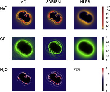
Untwisted ion and water normalized density distributions at 0.17 M NaCl. Results from MD with SPC/E (left), 3D-RISM-PSE-4 (middle), and NLPB (right) for sodium (upper row), chloride (middle row), and water oxygen (lower row). Due to the continuum treatment of the water dielectric effect, it is not possible to determine the distribution of water from NLPB theory in a straightforward manner.
Interaction with phosphates
Interactions between cations and phosphates outside the grooves have the largest impact on the shape of the molecular distribution functions and on estimated values of PIPs (see next section). The most important interactions relevant for ion-counting measurements are those between cation phosphate oxygen atoms. Isosurfaces derived from 3D distribution functions show that the binding patterns of cations to the phosphates fits the territorial binding picture with a multitude of binding patterns, making direct contact or sitting at one or two solvation layers away from the phosphates. There are not many sources of structural experimental data that can expose the detailed distributions of both ions and water in the immediate vicinity of helical nucleic acids. Anomalous small-angle x-ray scattering (2,3), for example, can be used to model the RDF between the electronic density of the nucleic acid and the excess number of surrounding ions out of scattering profiles, but no measurement has been made on a system such as that used in this work.
Ions residing outside the grooves but in the immediate vicinity of phosphates are included in region 3 of the cRDF (see Fig. 5), exhibiting a peak at ∼10 Å from the helical axis. The 3D-RISM yields the largest peak height, followed by MD simulations and finally NLPB calculations, which reveal a broad unstructured distribution. In addition, 3D-RISM distribution has the tightest shape.
Again, the untwisted densities provide insight into the interaction patterns and reveal further differences between the three methods (Fig. 4). First, distributions from MD simulations and 3D-RISM are layered and show more cationic density accumulated around phosphates. That is not the case with conventional NLPB calculations, which predict almost uniform distribution of cations around phosphates and the grooves. Furthermore, NLPB calculations fail to reveal any layering to distinguish between inner- and outer-sphere coordination between phosphates and sodiums. Second, one can explain the subtle differences between cRDFs originating from MD simulations and those from 3D-RISM (see Fig. 5). The 3D-RISM predicts a higher and more uniform accumulation of cations that make inner-sphere contacts than does MD simulation, as can be seen in the untwisted densities in region 5 of Fig. 3. MD predicts a higher density of cations making inner-sphere contacts around the minor groove. Further, for cations sitting at solvent separation from the phosphates (Fig. 3, region 8), MD simulation shows a higher density than 3D-RISM.
Correlation radius
The effect of the highly negatively charged nucleic acid on the cation distribution extends beyond the region where cations make inner- or outer-sphere contacts with the phosphates. In Fig. 5, one can observe that the sodium ion densities located outside of region 3 of cylindrical RDFs are different from those of the bulk for 10–20 Å more, depending on the salt concentration. As such, the correlation radius of the B-DNA molecule extends 25–35 Å away from its helical axis. As shown in Fig. 5, MD simulations, 3D-RISM, and NLPB calculations suggest that the correlation radius of the B-DNA molecule increases with decreasing monovalent salt concentration: at 0.7–0.8 M NaCl one can estimate a correlation radius of 25–28 Å, and at 0.1–0.2 M the value increases to 35 Å.
Preferential Interaction Parameters (PIPs)
Here we compare the estimates of ion counting from MD simulations, 3D-RISM, NLPB calculations, and experiment. Overall, we find that MD simulations and 3D-RISM are able to match results of ion-counting experiments over a range of concentrations, whereas NLPB calculations cannot (see Fig. 6 and Table S4). Good agreement between MD simulations and experiment has been found in recent studies on RNA duplexes (28,29). It is important to note in making this comparison that the estimated error in experimental results increases considerably with salt concentration. This is reflected in the net charge of the Na+ and Cl− (not shown), which is within error of 46 e but can deviate by several units.
Figure 6.
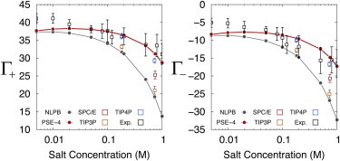
Comparison between theoretical estimates of Na+ (left) and Cl− (right) PIPs and experimental results from Bai et al. (4). To see this figure in color, go online.
For concentrations close to the physiological value, all MD estimates match experimental results within error but begin to fail at higher concentrations. In general, the calculations that use TIP4P-Ew and SPC/E water models are closest to experiment. TIP4P-Ew, in particular, is within or near experimental error for both Na+ and Cl−. SPC/E is close to experimental error for Cl− only and TIP3P provides excess numbers that are too low. At 0.2 M, SPC/E and TIP4P-Ew are nearly indistinguishable at 0.2 M, whereas TIP3P gives a lower result. The fact that 0.2 M is near the ideal ion regime is likely a significant contributor to the success of the various models at this concentration. For 0.73 M, only TIP4P-Ew has reasonable agreement with the experimental PIPs for both Na+ and Cl−. SPC/E is nearly within error for the Cl− PIP but falls well short of the Na+ value. TIP3P greatly underestimates the number of excess Na+ at this higher concentration. The larger van der Waals radius for Na+ in JC:TIP3P relative to the other parameter sets is a likely contributor to this result.
The 3D-RISM has good agreement with experimental results for all but the lowest concentrations. It also agrees well with SPC/E MD simulations at 0.1842 M but not at 0.7452 M. As noted in 4.1.1, when compared with MD simulations, 3D-RISM calculations underestimate the minor- and major-groove binding of ions and instead preferentially place ions around the phosphate backbone.
The NLPB model, on the other hand, fails over almost the entire concentration range. This was not evident in some previous studies (4,29) due to the method of calculating the number of excess ions and the ion radii that were used. As discussed in 2.1, when calculating PIPs in molar concentration units, it is important to integrate over the entire volume, including the solvent-excluded region in the DNA interior, when using Eqs. 6 and 16. For example, at 1 M, a volume equivalent to the ion-excluded region of the 24L DNA fragment in our NLPB calculations contains Na+. Omitting the ion-excluded region from the integral gives a PIP of rather than calculated from the all-space integral. Previous studies using NLPB methods have generally omitted the ion-excluded volume from PIP calculations and, combined with their use of large ion radii, have achieved good fits to experimental molar data. The ion radii used were typically Å, which is equivalent to having ions completely solvent-separated from the DNA surface. In contrast, MD simulations and 3D-RISM show ions in direct contact with DNA (see Fig. 4). Regardless of whether adjusting parameters would allow NLPB to obtain better agreement with ion-counting experiments, it is clear that the ion distributions using NLPB qualitatively lack structural details that are available only when correlation between solution components is considered.
Conclusions
The ion atmosphere around nucleic acids has tremendous importance for supporting structure, dynamics, or catalytic activity. Neutralization of the high and extended charge density of nucleic acids when they are brought into an aqueous environment is realized through two mechanisms: counterion condensation and anion depletion. Simulations can complement structural data extracted from x-ray, NMR, SAXS, and other measurements, and can provide an atomic-level description of the dynamics associated with the accumulation of ions around nucleic acids.
Herein, the results of MD simulations and 3D-RISM and NLPB calculations are analyzed and compared with available ion-counting measurements. The results for the NLPB model are markedly different from those of the two molecular-based theories. The net association of counterions is much smaller than with either the other theories or experiment at salt concentrations >0.4 M. However, regardless of the ion-counting numbers, the ion distributions themselves from NLPB are qualitatively inconsistent (at all concentrations studied here) with those from MD or 3D-RISM models, since the former all but lack any defined structure. These comparisons point to real limitations in the use of continuum solvent models in this field.
We present two methods to compute PIPs. The first approach uses KB integrals and depends on the local density of salt and water around the solute. The second approach uses two distinct spatial partitions, similar in spirit to the setup in osmosis experiments. In this case, one can estimate the PIPs by knowing the bulk concentrations of salt and water only. This approach might be well suited for irregularly shaped or flexible solutes for which distribution function might be harder to define.
At salt concentrations close to physiological values, the estimates for ion counting from MD and 3D-RISM are within error of the experimentally determined values. The ion distributions from MD simulations and 3D-RISM calculations, from which PIPs are computed, are largely compatible, clearly showing a multilayered distribution and distinct ionic binding sites in the major and minor grooves. However, there are some discrepancies in the details of these distributions, such as the propensity of 3D-RISM to overaccumulate sodiums around the phosphate backbone, its slightly reduced density maxima, and its overrepresentation of chlorides near the DNA surface. At concentrations close to 1 M, MD simulations and 3D-RISM calculations underestimate the values, with JC:TIP4PEw and JC:SPC/E parameter sets being closer to experiment.
These results provide an overall picture of how simple helical nucleic acids are neutralized by the ion atmosphere in electrolyte solutions. The distribution of ions and water is layered outside the grooves and has well defined, sequence-dependent competing binding modes in both the minor and major grooves. The results presented here lay the ground for future efforts to improve the representation of DNA-ion interactions over larger concentration ranges, and to begin to dissect the contribution of the ion atmosphere in RNA folding.
Acknowledgments
This work used the Extreme Science and Engineering Discovery Environment (XSEDE), which is supported by National Science Foundation grant number OCI-1053575. We thank Lois Pollack for many useful discussions.
This work was supported by National Institutes of Health grants GM57513, GM103297(D.A.C.), and P01GM066275(D.M.Y. and D.H.).
Footnotes
George M. Giambaşu and Tyler Luchko contributed equally to this work.
Tyler Luchko’s present address is Department of Physics and Astronomy, California State University Northridge, Northridge, CA 91330.
Contributor Information
Darrin M. York, Email: york@biomaps.rutgers.edu.
David A. Case, Email: case@biomaps.rutgers.edu.
Supporting Material
References
- 1.Draper D.E., Grilley D., Soto A.M. Ions and RNA folding. Annu. Rev. Biophys. Biomol. Struct. 2005;34:221–243. doi: 10.1146/annurev.biophys.34.040204.144511. [DOI] [PubMed] [Google Scholar]
- 2.Pabit S.A., Meisburger S.P., Pollack L. Counting ions around DNA with anomalous small-angle x-ray scattering. J. Am. Chem. Soc. 2010;132:16334–16336. doi: 10.1021/ja107259y. [DOI] [PMC free article] [PubMed] [Google Scholar]
- 3.Pollack L. SAXS studies of ion-nucleic acid interactions. Annu. Rev. Biophys. 2011;40:225–242. doi: 10.1146/annurev-biophys-042910-155349. [DOI] [PubMed] [Google Scholar]
- 4.Bai Y., Greenfeld M., Herschlag D. Quantitative and comprehensive decomposition of the ion atmosphere around nucleic acids. J. Am. Chem. Soc. 2007;129:14981–14988. doi: 10.1021/ja075020g. [DOI] [PMC free article] [PubMed] [Google Scholar]
- 5.Greenfeld M., Herschlag D. Probing nucleic acid-ion interactions with buffer exchange-atomic emission spectroscopy. Methods Enzymol. 2009;469:375–389. doi: 10.1016/S0076-6879(09)69018-2. [DOI] [PubMed] [Google Scholar]
- 6.Grilley D., Soto A.M., Draper D.E. Mg2+-RNA interaction free energies and their relationship to the folding of RNA tertiary structures. Proc. Natl. Acad. Sci. USA. 2006;103:14003–14008. doi: 10.1073/pnas.0606409103. [DOI] [PMC free article] [PubMed] [Google Scholar]
- 7.Bleam M.L., Anderson C.F., Record M.T., Jr. Relative binding affinities of monovalent cations for double-stranded DNA. Proc. Natl. Acad. Sci. USA. 1980;77:3085–3089. doi: 10.1073/pnas.77.6.3085. [DOI] [PMC free article] [PubMed] [Google Scholar]
- 8.Braunlin W.H., Anderson C.F., Record M.T., Jr. Competitive interactions of Co(NH3)63+ and Na+ with helical B-DNA probed by 59Co and 23Na NMR. Biochemistry. 1987;26:7724–7731. doi: 10.1021/bi00398a028. [DOI] [PubMed] [Google Scholar]
- 9.Lyubartsev A.P. Molecular simulations of DNA counterion distributions. In: Schwarz J.A., Lyshevski S.E., Putyera K., Contescu C., editors. Dekker Encyclopedia of Nanoscience and Nanotechnology. CRC Press; Boca Raton, FL: 2004. pp. 2131–2143. [Google Scholar]
- 10.Ponomarev S.Y., Thayer K.M., Beveridge D.L. Ion motions in molecular dynamics simulations on DNA. Proc. Natl. Acad. Sci. USA. 2004;101:14771–14775. doi: 10.1073/pnas.0406435101. [DOI] [PMC free article] [PubMed] [Google Scholar]
- 11.Manning G.S. Counterion binding in polyelectrolyte theory. Acc. Chem. Res. 1979;12:443–449. [Google Scholar]
- 12.Manning G.S. The molecular theory of polyelectrolyte solutions with applications to the electrostatic properties of polynucleotides. Q. Rev. Biophys. 1978;11:179–246. doi: 10.1017/s0033583500002031. [DOI] [PubMed] [Google Scholar]
- 13.Anderson C.F., Record M.T., Jr. Salt-nucleic acid interactions. Annu. Rev. Phys. Chem. 1995;46:657–700. doi: 10.1146/annurev.pc.46.100195.003301. [DOI] [PubMed] [Google Scholar]
- 14.Manning G.S. A counterion condensation theory for the relaxation, rise, and frequency dependence of the parallel polarization of rodlike polyelectrolytes. Eur Phys J E Soft Matter. 2011;34:1–7. doi: 10.1140/epje/i2011-11039-2. [DOI] [PubMed] [Google Scholar]
- 15.Manning G.S. Counterion condensation on charged spheres, cylinders, and planes. J. Phys. Chem. B. 2007;111:8554–8559. doi: 10.1021/jp0670844. [DOI] [PubMed] [Google Scholar]
- 16.Manning G.S. Electrostatic free energies of spheres, cylinders, and planes in counterion condensation theory with some applications. Macromolecules. 2007;40:8071–8081. [Google Scholar]
- 17.Draper D.E. RNA folding: thermodynamic and molecular descriptions of the roles of ions. Biophys. J. 2008;95:5489–5495. doi: 10.1529/biophysj.108.131813. [DOI] [PMC free article] [PubMed] [Google Scholar]
- 18.Chen A.A., Draper D.E., Pappu R.V. Molecular simulation studies of monovalent counterion-mediated interactions in a model RNA kissing loop. J. Mol. Biol. 2009;390:805–819. doi: 10.1016/j.jmb.2009.05.071. [DOI] [PMC free article] [PubMed] [Google Scholar]
- 19.Kirmizialtin S., Elber R. Computational exploration of mobile ion distributions around RNA duplex. J. Phys. Chem. B. 2010;114:8207–8220. doi: 10.1021/jp911992t. [DOI] [PMC free article] [PubMed] [Google Scholar]
- 20.Korolev N., Lyubartsev A.P., Nordenskiöld L. A molecular dynamics simulation study of oriented DNA with polyamine and sodium counterions: diffusion and averaged binding of water and cations. Nucleic Acids Res. 2003;31:5971–5981. doi: 10.1093/nar/gkg802. [DOI] [PMC free article] [PubMed] [Google Scholar]
- 21.Rueda M., Cubero E., Orozco M. Exploring the counterion atmosphere around DNA: what can be learned from molecular dynamics simulations? Biophys. J. 2004;87:800–811. doi: 10.1529/biophysj.104.040451. [DOI] [PMC free article] [PubMed] [Google Scholar]
- 22.Sen S., Andreatta D., Berg M.A. Dynamics of water and ions near DNA: comparison of simulation to time-resolved Stokes-shift experiments. J. Am. Chem. Soc. 2009;131:1724–1735. doi: 10.1021/ja805405a. [DOI] [PMC free article] [PubMed] [Google Scholar]
- 23.Chen A.A., Marucho M., Pappu R.V. Simulations of RNA interactions with monovalent ions. Methods Enzymol. 2009;469:411–432. doi: 10.1016/S0076-6879(09)69020-0. [DOI] [PubMed] [Google Scholar]
- 24.Bonvin A.M. Localisation and dynamics of sodium counterions around DNA in solution from molecular dynamics simulation. Eur. Biophys. J. 2000;29:57–60. doi: 10.1007/s002490050251. [DOI] [PubMed] [Google Scholar]
- 25.Dai L., Mu Y., van der Maarel J.R. Molecular dynamics simulation of multivalent-ion mediated attraction between DNA molecules. Phys. Rev. Lett. 2008;100:118301. doi: 10.1103/PhysRevLett.100.118301. [DOI] [PubMed] [Google Scholar]
- 26.Luan B., Aksimentiev A. DNA attraction in monovalent and divalent electrolytes. J. Am. Chem. Soc. 2008;130:15754–15755. doi: 10.1021/ja804802u. [DOI] [PMC free article] [PubMed] [Google Scholar]
- 27.Noy A., Soteras I., Orozco M. The impact of monovalent ion force field model in nucleic acids simulations. Phys. Chem. Chem. Phys. 2009;11:10596–10607. doi: 10.1039/b912067j. [DOI] [PubMed] [Google Scholar]
- 28.Kirmizialtin S., Pabit S.A., Elber R. RNA and its ionic cloud: solution scattering experiments and atomically detailed simulations. Biophys. J. 2012;102:819–828. doi: 10.1016/j.bpj.2012.01.013. [DOI] [PMC free article] [PubMed] [Google Scholar]
- 29.Kirmizialtin S., Silalahi A.R.J., Fenley M.O. The ionic atmosphere around A-RNA: Poisson-Boltzmann and molecular dynamics simulations. Biophys. J. 2012;102:829–838. doi: 10.1016/j.bpj.2011.12.055. [DOI] [PMC free article] [PubMed] [Google Scholar]
- 30.Auffinger P., Westhof E. Water and ion binding around RNA and DNA (C,G) oligomers. J. Mol. Biol. 2000;300:1113–1131. doi: 10.1006/jmbi.2000.3894. [DOI] [PubMed] [Google Scholar]
- 31.Yoo J., Aksimentiev A. Improved parametrization of Li+, Na+, K+, and Mg++ ions for all-atom molecular dynamics simulations of nucleic acid systems. J. Phys. Chem. Lett. 2012;3:45–50. [Google Scholar]
- 32.Auffinger P., Westhof E. Water and ion binding around r(UpA)12 and d(TpA)12 oligomers—comparison with RNA and DNA (CpG)12 duplexes. J. Mol. Biol. 2001;305:1057–1072. doi: 10.1006/jmbi.2000.4360. [DOI] [PubMed] [Google Scholar]
- 33.Chu V.B., Bai Y., Doniach S. Evaluation of ion binding to DNA duplexes using a size-modified Poisson-Boltzmann theory. Biophys. J. 2007;93:3202–3209. doi: 10.1529/biophysj.106.099168. [DOI] [PMC free article] [PubMed] [Google Scholar]
- 34.Pabit S.A., Qiu X., Pollack L. Both helix topology and counterion distribution contribute to the more effective charge screening in dsRNA compared with dsDNA. Nucleic Acids Res. 2009;37:3887–3896. doi: 10.1093/nar/gkp257. [DOI] [PMC free article] [PubMed] [Google Scholar]
- 35.Bond J.P., Anderson C.F., Record M.T., Jr. Conformational transitions of duplex and triplex nucleic acid helices: thermodynamic analysis of effects of salt concentration on stability using preferential interaction coefficients. Biophys. J. 1994;67:825–836. doi: 10.1016/S0006-3495(94)80542-9. [DOI] [PMC free article] [PubMed] [Google Scholar]
- 36.Gonzales-Tovar E., Lozada-Cassou M., Henderson D. Hypernetted chain approximation for the distribution of ions around a cylindrical electrode. II. Numerical solution for a model cylindrical polyelectrolyte. J. Chem. Phys. 1985;83:361–372. [Google Scholar]
- 37.Maruyama Y., Yoshida N., Hirata F. Revisiting the salt-induced conformational change of DNA with 3D-RISM theory. J. Phys. Chem. B. 2010;114:6464–6471. doi: 10.1021/jp912141u. [DOI] [PubMed] [Google Scholar]
- 38.Howard J.J., Lynch G.C., Pettitt B.M. Ion and solvent density distributions around canonical B-DNA from integral equations. J. Phys. Chem. B. 2011;115:547–556. doi: 10.1021/jp107383s. [DOI] [PMC free article] [PubMed] [Google Scholar]
- 39.Maruyama Y., Matsushita T., Hirata F. Solvent and salt effects on structural stability of human telomere. J. Phys. Chem. B. 2011;115:2408–2416. doi: 10.1021/jp1096019. [DOI] [PubMed] [Google Scholar]
- 40.Beglov D., Roux B. An integral equation to describe the solvation of polar molecules in liquid water. J. Phys. Chem. B. 1997;101:7821–7826. [Google Scholar]
- 41.Kovalenko A., Hirata F. Self-consistent description of a metal-water interface by the Kohn-Sham density functional theory and the three-dimensional reference interaction site model. J. Chem. Phys. 1999;110:10095–10112. [Google Scholar]
- 42.Kovalenko A., Hirata F. Potentials of mean force of simple ions in ambient aqueous solution. I. Three-dimensional reference interaction site model approach. J. Chem. Phys. 2000;112:10391–10402. [Google Scholar]
- 43.Kovalenko A. Three-dimensional RISM theory for molecular liquids and solid-liquid interfaces. In: Hirata F., editor. Molecular Theory of Solvation. Kluwer Academic; Norwell, MA: 2003. pp. 265–268. [Google Scholar]
- 44.Luchko T., Gusarov S., Kovalenko A. Three-dimensional molecular theory of solvation coupled with molecular dynamics in Amber. J. Chem. Theory Comput. 2010;6:607–624. doi: 10.1021/ct900460m. [DOI] [PMC free article] [PubMed] [Google Scholar]
- 45.Leipply D., Lambert D., Draper D.E. Ion-RNA interactions thermodynamic analysis of the effects of mono- and divalent ions on RNA conformational equilibria. Methods Enzymol. 2009;469:433–463. doi: 10.1016/S0076-6879(09)69021-2. [DOI] [PMC free article] [PubMed] [Google Scholar]
- 46.Record M.T., Jr., Anderson C.F. Interpretation of preferential interaction coefficients of nonelectrolytes and of electrolyte ions in terms of a two-domain model. Biophys. J. 1995;68:786–794. doi: 10.1016/S0006-3495(95)80254-7. [DOI] [PMC free article] [PubMed] [Google Scholar]
- 47.Shulgin I.L., Ruckenstein E. A protein molecule in a mixed solvent: the preferential binding parameter via the Kirkwood-Buff theory. Biophys. J. 2006;90:704–707. doi: 10.1529/biophysj.105.074112. [DOI] [PMC free article] [PubMed] [Google Scholar]
- 48.Smith P.E. Equilibrium dialysis data and the relationships between preferential interaction parameters for biological systems in terms of Kirkwood-Buff integrals. J. Phys. Chem. B. 2006;110:2862–2868. doi: 10.1021/jp056100e. [DOI] [PubMed] [Google Scholar]
- 49.Anderson C.F., Record M.T., Jr. Ion distributions around DNA and other cylindrical polyions: theoretical descriptions and physical implications. Annu. Rev. Biophys. Biophys. Chem. 1990;19:423–465. doi: 10.1146/annurev.bb.19.060190.002231. [DOI] [PubMed] [Google Scholar]
- 50.Anderson C.F., Record M.T., Jr. Polyelectrolyte theories and their applications to DNA. Annu. Rev. Phys. Chem. 1982;33:191–222. [Google Scholar]
- 51.Hansen J.-P., McDonald I.R. 2nd ed. Academic Press; London: 1990. Theory of Simple Liquids; pp. 97–144. [Google Scholar]
- 52.Chitra R., Smith P.E. Properties of 2,2,2-trifluoroethanol and water mixtures. J. Chem. Phys. 2001;114:426–435. [Google Scholar]
- 53.Ben-Naim A. Plenum Press; New York: 1992. Statistical Thermodynamics for Chemists and Biochemists. [Google Scholar]
- 54.Smith P.E. Cosolvent interactions with biomolecules: relating computer simulation data to experimental thermodynamic data. J. Phys. Chem. B. 2004;108:18716–18724. [Google Scholar]
- 55.Ben-Naim A. Oxford University Press; New York: 2006. Molecular Theory of Solutions. [Google Scholar]
- 56.Record M.T., Jr., Zhang W., Anderson C.F. Analysis of effects of salts and uncharged solutes on protein and nucleic acid equilibria and processes: a practical guide to recognizing and interpreting polyelectrolyte effects, Hofmeister effects, and osmotic effects of salts. Adv. Protein Chem. 1998;51:281–353. doi: 10.1016/s0065-3233(08)60655-5. [DOI] [PubMed] [Google Scholar]
- 57.Macke T.J., Case D.A. Modeling unusual nucleic acid structures. In: Leontis N.B., SantaLucia J., editors. Molecular Modeling of Nucleic Acids. American Chemical Society; Washington, D.C: 1997. pp. 379–393. [Google Scholar]
- 58.Arnott S., Hukins D.W.L. Optimised parameters for A-DNA and B-DNA. Biochem. Biophys. Res. Commun. 1972;47:1504–1509. doi: 10.1016/0006-291x(72)90243-4. [DOI] [PubMed] [Google Scholar]
- 59.Jorgensen W.L., Chandrasekhar J., Klein M.L. Comparison of simple potential functions for simulating liquid water. J. Chem. Phys. 1983;79:926–935. [Google Scholar]
- 60.Horn H.W., Swope W.C., Head-Gordon T. Development of an improved four-site water model for biomolecular simulations: TIP4P-Ew. J. Chem. Phys. 2004;120:9665–9678. doi: 10.1063/1.1683075. [DOI] [PubMed] [Google Scholar]
- 61.Horn H.W., Swope W.C., Pitera J.W. Characterization of the TIP4P-Ew water model: vapor pressure and boiling point. J. Chem. Phys. 2005;123:194504. doi: 10.1063/1.2085031. [DOI] [PubMed] [Google Scholar]
- 62.Berendsen H.J.C., Grigera J.R., Straatsma T.P. The missing term in effective pair potentials. J. Phys. Chem. 1987;91:6269–6271. [Google Scholar]
- 63.Joung I.S., Luchko T., Case D.A. Simple electrolyte solutions: comparison of DRISM and molecular dynamics results for alkali halide solutions. J. Chem. Phys. 2013;138:044103. doi: 10.1063/1.4775743. [DOI] [PMC free article] [PubMed] [Google Scholar]
- 64.Joung I.S., Cheatham T.E., 3rd Determination of alkali and halide monovalent ion parameters for use in explicitly solvated biomolecular simulations. J. Phys. Chem. B. 2008;112:9020–9041. doi: 10.1021/jp8001614. [DOI] [PMC free article] [PubMed] [Google Scholar]
- 65.Pérez A., Marchán I., Orozco M. Refinement of the AMBER force field for nucleic acids: improving the description of α/γ conformers. Biophys. J. 2007;92:3817–3829. doi: 10.1529/biophysj.106.097782. [DOI] [PMC free article] [PubMed] [Google Scholar]
- 66.Banáš P., Hollas D., Otyepka M. Performance of molecular mechanics force fields for RNA simulations: stability of UUCG and GNRA hairpins. J. Chem. Theory Comput. 2010;6:3836–3849. doi: 10.1021/ct100481h. [DOI] [PMC free article] [PubMed] [Google Scholar]
- 67.Wang J., Cieplak P., Kollman P.A. How well does a restrained electrostatic potential (RESP) model perform in calcluating conformational energies of organic and biological molecules? J. Comput. Chem. 2000;21:1049–1074. [Google Scholar]
- 68.Case D.A., Darden T.A., Kollman P.A. San Francisco; San Francisco: 2002. AMBER 10. University of California. [Google Scholar]
- 69.Pearlman D.A., Case D.A., Kollman P. AMBER, a package of computer programs for applying molecular mechanics, normal mode analysis, molecular dynamics and free energy calculations to simulate the structure and energetic properties of molecules. Comput. Phys. Commun. 1995;91:1–41. [Google Scholar]
- 70.Case D.A., Cheatham T.E., 3rd, Woods R.J. The Amber biomolecular simulation programs. J. Comput. Chem. 2005;26:1668–1688. doi: 10.1002/jcc.20290. [DOI] [PMC free article] [PubMed] [Google Scholar]
- 71.Phillips J.C., Braun R., Schulten K. Scalable molecular dynamics with NAMD. J. Comput. Chem. 2005;26:1781–1802. doi: 10.1002/jcc.20289. [DOI] [PMC free article] [PubMed] [Google Scholar]
- 72.Martyna G.J., Tobias D.J., Klein M.L. Constant pressure molecular dynamics algorithms. J. Chem. Phys. 1994;101:4177–4189. [Google Scholar]
- 73.Feller S.E., Zhang Y., Brooks B.R. Constant pressure molecular dynamics simulation: the Langevin piston method. J. Chem. Phys. 1995;103:4613–4621. [Google Scholar]
- 74.Essmann U., Perera L., Pedersen L.G. A smooth particle mesh Ewald method. J. Chem. Phys. 1995;103:8577–8593. [Google Scholar]
- 75.Sagui C., Darden T.A. Molecular dynamics simulations of biomolecules: long-range electrostatic effects. Annu. Rev. Biophys. Biomol. Struct. 1999;28:155–179. doi: 10.1146/annurev.biophys.28.1.155. [DOI] [PubMed] [Google Scholar]
- 76.Allen M.P., Tildesley D.J. Clarendon Press; Oxford, United Kingdom: 1987. Computer Simulation of Liquids. [Google Scholar]
- 77.Ryckaert J.P., Ciccotti G., Berendsen H.J.C. Numerical integration of the Cartesian equations of motion of a system with constraints: molecular dynamics of n-alkanes. J. Comput. Phys. 1977;23:327–341. [Google Scholar]
- 78.Ornstein L.S., Zernike F. Accidental deviations of density and opalescence at the critical point of a single substance. Proc. Akad. Sci. Amsterdam. 1914;17:793–806. [Google Scholar]
- 79.Ornstein L.S., Zernike F. The Equilibrium Theory of Classical Fluids: A Lecture Note and Reprint Volume. W. A. Benjamin; New York: 1964. Accidental deviations of density and opalescence at the critical point of a single substance; pp. 2–16. [Google Scholar]
- 80.Perkyns J.S., Pettitt B.M. A dielectrically consistent interaction site theory for solvent-electrolyte mixtures. Chem. Phys. Lett. 1992;190:626–630. [Google Scholar]
- 81.Perkyns J.S., Pettitt B.M. A site-site theory for finite concentration saline solutions. J. Chem. Phys. 1992;97:7656–7666. [Google Scholar]
- 82.Springer J.F., Pokrant M.A., Stevens F.A. Integral equation solutions for the classical electron gas. J. Chem. Phys. 1973;58:4863–4867. [Google Scholar]
- 83.Abernethy G.M., Gillan M.J. A new method of solving the HNC equation for ionic liquids. Mol. Phys. 1980;39:839–847. [Google Scholar]
- 84.Ng K. Hypernetted chain solutions for the classical one-component plasma up to Γ = 7000. J. Chem. Phys. 1974;61:2680–2689. [Google Scholar]
- 85.Kinoshita M., Hirata F. Application of the reference interaction site model theory to analysis on surface-induced structure of water. J. Chem. Phys. 1996;104:8807–8815. [Google Scholar]
- 86.Perkyns J.S., Lynch G.C., Pettitt B.M. Protein solvation from theory and simulation: exact treatment of Coulomb interactions in three-dimensional theories. J. Chem. Phys. 2010;132:064106. doi: 10.1063/1.3299277. [DOI] [PMC free article] [PubMed] [Google Scholar]
- 87.Gusarov S., Pujari B.S., Kovalenko A. Efficient treatment of solvation shells in 3D molecular theory of solvation. J. Comput. Chem. 2012;33:1478–1494. doi: 10.1002/jcc.22974. [DOI] [PubMed] [Google Scholar]
- 88.Morita T. Theory of classical fluids: hypernetted chain approximation. I. Formulation for a one-component system. Prog. Theor. Phys. 1958;20:920–928. [Google Scholar]
- 89.Rasaiah J.C., Card D.N., Valleau J.P. Calculations on the “restricted primitive model” for 1–1 electrolyte solutions. J. Chem. Phys. 1972;56:248–255. [Google Scholar]
- 90.Hansen J.P., McDonald I.R. Statistical mechanics of dense ionized matter. IV. Density and charge fluctuations in a simple molten salt. Phys. Rev. A. 1975;11:2111–2123. [Google Scholar]
- 91.Pettitt B.M., Rossky P.J. Integral equation predictions of liquid state structure for waterlike intermolecular potentials. J. Chem. Phys. 1982;77:1451–1457. [Google Scholar]
- 92.Hirata F., Rossky P.J. An extended RISM equation for molecular polar fluids. Chem. Phys. Lett. 1981;83:329–334. [Google Scholar]
- 93.Hirata F., Pettitt B.M., Rossky P.J. Application of an extended RISM equation to dipolar and quadrupolar fluids. J. Chem. Phys. 1982;77:509–520. [Google Scholar]
- 94.Singer S.J., Chandler D. Free-energy functions in the extended RISM approximation. Mol. Phys. 1985;55:621–625. [Google Scholar]
- 95.Kast S.M., Kloss T. Closed-form expressions of the chemical potential for integral equation closures with certain bridge functions. J. Chem. Phys. 2008;129:236101. doi: 10.1063/1.3041709. [DOI] [PubMed] [Google Scholar]
- 96.Case D.A., Darden T.A., Kollman P.A. University of California; San Francisco, CA: 2012. AMBER 12. [Google Scholar]
- 97.Kovalenko A., Ten-no S., Hirata F. Solution of three-dimensional reference interaction site model and hypernetted chain equations for simple point charge water by modified method of direct inversion in iterative subspace. J. Comput. Chem. 1999;20:928–936. [Google Scholar]
- 98.Söhnel O., Novotný P. Elsevier; Munich: 1985. Densities of Aqueous Solutions of Inorganic Substances. [Google Scholar]
- 99.Millero F.J. The apparent and partial molal volume of aqueous sodium chloride solutions at various temperatures. J. Phys. Chem. 1970;74:356–362. [Google Scholar]
- 100.Honig B., Nicholls A. Classical electrostatics in biology and chemistry. Science. 1995;268:1144–1149. doi: 10.1126/science.7761829. [DOI] [PubMed] [Google Scholar]
- 101.Simonson T. Electrostatics and dynamics of proteins. Rep. Prog. Phys. 2003;66:737–787. [Google Scholar]
- 102.Baker N.A., Sept D., McCammon J.A. Electrostatics of nanosystems: application to microtubules and the ribosome. Proc. Natl. Acad. Sci. USA. 2001;98:10037–10041. doi: 10.1073/pnas.181342398. [DOI] [PMC free article] [PubMed] [Google Scholar]
- 103.Neidle S. Academic Press; New York: 2008. Principles of Nucleic Acid Structure. [Google Scholar]
- 104.Blackburn G.M., Gait M.J., Williams D.M. Oxford University Press; New York: 2006. Nucleic Acids in Chemistry and Biology. [Google Scholar]
- 105.Sigel A., Sigel H., Sigel R.K.O. Springer; Dordrecht, The Netherlands: 2012. Interplay between Metal Ions and Nucleic Acids. [Google Scholar]
Associated Data
This section collects any data citations, data availability statements, or supplementary materials included in this article.