

Abstract
Survival analysis endures as an old, yet active research field with applications that spread across many domains. Continuing improvements in data acquisition techniques pose constant challenges in applying existing survival analysis methods to these emerging data sets. In this paper, we present tools for fitting regularized Cox survival analysis models on high-dimensional, massive sample-size (HDMSS) data using a variant of the cyclic coordinate descent optimization technique tailored for the sparsity that HDMSS data often present. Experiments on two real data examples demonstrate that efficient analyses of HDMSS data using these tools result in improved predictive performance and calibration.
Keywords: Big data, Cox proportional hazards, Regularized regression, Survival analysis
1. Introduction
Survival analysis characterizes relationships between time-to-event endpoints and multiple explanatory variables (covariates) (Kalbfleisch and Prentice, 1980; Oakes, 2001). Historically, the event of interest in survival analysis is patient death, but active research in the field over the past few decades provides applications spread across many domains including biostatistics, sociology, economics, demography, and engineering (Heckman and Singer, 1985; Collett, 2003; Box-Steffensmeier and Jones, 2004; Hosmer and others, 2008). Until recently, survival analyses have been limited to applications with only a handful of predictors and a few hundreds or thousands of observations. However, recent advances in data acquisition techniques and the ease of access to high computation power have fueled increased interest in analyzing data with potentially hundreds of thousands of variables and even millions of observations. For example, new technologies in genomics produce high-dimensional (HD) microarray gene expression data where the number of predictor variables is of the order of 105 or more. Other large-scale applications include medical adverse event monitoring, longitudinal clinical trials, and business data mining tasks. In these applications, the number of observations often far exceeds 106. So, they all require methods for analyzing HD, massive sample-size (HDMSS) data in a survival analysis framework.
Since its introduction, the Cox proportional hazards model (Cox, 1972) has reigned over algorithmic and applied research for analyzing time-to-event data. Unlike several fully parametric models (Collett, 2003; Klein and Moeschberger, 2003; Hosmer and others, 2008), the Cox model offers greater flexibility due to its semi-parametric nature but still yields regression coefficients that are readily interpretable. Typically, one obtains a Cox model fit by maximizing its partial likelihood. A regularized approach adds a complexity penalty to this likelihood with one version that favors sparseness in the fitted model leading to the point estimates for many of the model parameters being shrunk to zero. To this end, Park and Hastie (2007), Sohn and others (2009), and Goeman (2010) have proposed several different implementations of regularized Cox models. Although these implementations work well for small-scale problems, they do not scale well to HDMSS data due to their use of costly Newton–Raphson iterations that require inverting large matrices. Possible workarounds and approximations often lead to large estimated coefficient variances, numerical ill-conditioning, and poor predictive accuracy or calibration.
In this paper, we describe a regularized approach to Cox survival modeling that scales for HDMSS data. To solve the optimization problem, we exploit a variation of the cyclic coordinate descent optimization technique (Tseng, 2001; Genkin and others, 2007; Koh and others, 2007; Tibshirani and others, 2010; Suchard and others, 2013). We show that application of this tool to HDMSS data avoids overfitting, can provide improved predictive performance over corresponding low-dimensional (LD) models, and remains efficient both during fitting and prediction time.
In Section 2, we review some relevant related work. In Section 3, we describe the regularized Cox survival model and, in Section 4, we present our optimization technique that is tailored for tractably computing coefficient estimates through efficient implementation and storage. We describe the data sets that we use for our experiments in Section 5, and provide experimental results in Sections 6 and 7. Finally, we conclude in Section 8 with directions for future work.
2. Related work
Efforts to achieve HDMSS survival analysis has been two-fold—to develop new statistical methods for efficient data analysis (Shivaswamy and others, 2007; Evers and Messow, 2008; Ishwaran and others, 2010, 2011; Van Belle and others, 2011) and to extend the existing techniques to handle larger data sets (Engler and Li, 2009; Friedman and others, 2010; Goeman, 2010). For example, the work of Evers and Messow (2008) and Van Belle and others (2011) has extended the traditional supports vector machines used for classification to survival analysis by additionally penalizing discordant pairs of observations. Other methods like those used by Ishwaran and others (2010, 2011) extend the use of random forests for variable selection in survival analysis. Similarly, the method of Engler and Li (2009) uses an elastic net approach for variable selection for survival analysis models while the work of Goeman (2010) applies an efficient method to compute L1-penalized parameter estimates for Cox model. The recent review article of Witten and Tibshirani (2010) provides a survey of the existing techniques for variable selection and model estimation for HD survival analysis with moderate sample sizes.
Some more recent tools such as coxnet (Simon and others, 2011) and fastcox (Yang and Zou, 2012) adopt optimization approaches that can scale to HDMSS data. Neither coxnet nor fastcox currently support the requisite sparse matrix formats for the input data (although other models provided by the R package glmnet do support sparse formats). Both coxnet and fastcox provide L1 and elastic net regularized estimates under the Cox proportional hazards model.
3. Regularized Cox survival analysis
Assuming a typical survival analysis setting, let n be the number of individuals in the training data. We represent their survival times by  for
for  , where
  and
and  are the time-to-event (failure time) and right-censoring time for each individual. Let
  be the indicator variable such that
  equals 1 if the observation is not censored and 0 otherwise. Further, let
  be a p-vector of covariates for individual i. We assume that
  and
and  are conditionally independent given
  and that the censoring mechanism is non-informative. The observed data comprise triplets
  .
.
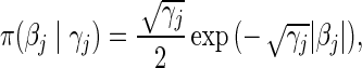
Let  be the p-vector of unknown, underlying model parameters. We assume that the survival times
  arise in an independent and identically distributed fashion from density and survival functions
  and
and  parameterized by
  , respectively. We are interested in the likelihood
  of the parametric model, where
 |
(3.1) |
The Cox proportional hazard model (Cox, 1972) posits a semi-parametric hazard function  of the form
 |
(3.2) |
where  represents the unspecified baseline hazard function and covariates relate multiplicatively to the hazard. Similarly, the survival function unfolds as
 |
(3.3) |
Through the parameterizations (3.2) and (3.3), the likelihood function of (3.1) falls out as
 |
(3.4) |
In the absence of explicit specification of the baseline hazard, it becomes hard to work with  directly. Alternatively, Cox (1972) proposes to maximize the partial likelihood function
 |
(3.5) |
where  represents the risk set of the ith observation; specifically,
  . Note the above expression assumes that there are no tied survival times. In practice, for HDMSS data, it suffices to break the ties by adding a small random quantity (uniform between [−10−5, 10−5]) to the event times. One can then estimate
  through the joint penalized partial likelihood
  , by assuming a penalty
  for
for  that shrinks the components of
  toward zero.
3.1. The L2 penalty and ridge regression
For the L2 penalty, we have
 |
(3.6) |
The regularization or tuning parameters  , are positive constants that control the degree of regularization and we choose them through cross-validation. Smaller values of
  imply stronger shrinkage of
  toward zero. Absent further knowledge, we typically assume that
  . This formulation is equivalent to performing ridge regression (Hoerl and Kennard, 1970) and generally it does not result in a sparse solution.
3.2. The L1 penalty and lasso regression
For the L1 penalty, we have
 |
(3.7) |
where  represent a vector of regularization or tuning parameters. Absent prior knowledge, we assume that
  and select a value using cross-validation. This formulation is equivalent to a lasso regression (Tibshirani, 1996). Using this approach, a sparse solution typically ensues, that is, many components of the estimated
  vector will be zero.
4. Finding the parameter estimates
The penalized partial likelihood of  in the L2 case can be written as
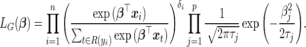 |
(4.1) |
Maximizing  is equivalent to maximizing
 |
(4.2) |
where the last negated sum is the penalty term. For the L1 case, we arrive at the penalized partial likelihood  by replacing the penalty term above with
  . For both L1 and L2 regularization, their respective negated log-penalized partial likelihoods are log-convex and a wide range of optimization algorithms can be utilized. However, due to the high dimensionality of our applications, usual methods like Newton–Raphson are not feasible owing to their high memory requirements and numerical instability. Many alternate optimization approaches exist for parameter estimation in HD, regularized, regression problems (Zhang and Oles, 2000; Kivinen and Warmuth, 2001). We use the column relaxation with logistic loss (CLG) algorithm of Zhang and Oles (2000), a type of cyclic coordinate descent algorithm, which provides the favorable property of scaling to HD data with ease of implementation (Wu and Lange, 2008; Simon and others, 2011; Gorst-Rasmussen and Scheike, 2012). Genkin and others (2007) adapt this method for performing large-scale logistic regression, implemented in the widely used BBR/BXR software (http://www.bayesianregression.org). More recently, Mittal and others (2013) use the method for fitting parametric survival analysis models and Suchard and others (2013) discuss how the approach scales to massive sample size data sets for generalized linear models.
A cyclic coordinate descent algorithm begins by setting all variables to some initial value. While holding all other variables constant, it then solves a 1D optimization problem to set the first variable to a value that minimizes or drives downhill the objective function. The algorithm then finds the minimizing value of a second variable, while holding all others constant (including the new value of the first variable). The third variable is then optimized, and so on. When all variables have been traversed, the algorithm returns to the first variable and starts again. Multiple passes are made over the variables until some convergence criterion is met. Since the CLG method relies on 1D updates, it does not need to compute, store, or invert an HD Hessian matrix. Below, we describe the details of the algorithm for minimizing the negated log-penalized partial likelihood for both L1 and L2 penalties. For more details on the CLG method, see Zhang and Oles (2000) or Genkin and others (2007).
Using the CLG algorithm, the 1D optimization problem involves finding  , the value of the jth entry of
  that minimizes
  , assuming that the other
  's are held at their current values. Therefore, using (4.2) in the L2 case (and ignoring the constants
  and
and  ), finding
  is equivalent to finding the z that minimizes
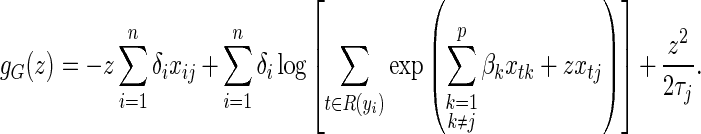 |
(4.3) |
The classic Newton method approximates the objective function  by the first three terms of its Taylor series at the current
  ,
,
 |
(4.4) |
where
 |
(4.5) |
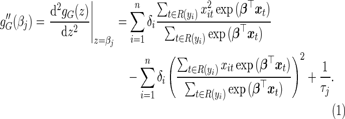 |
(4.6) |
Likewise, in the L1 case and  , we replace the last term in (4.5) with
  to arrive at
  and drop the last term in (4.6) to generate
  . The value of
  for both types of penalties can then be computed as
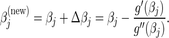 |
(4.7) |
For steps crossing the origin under the L1 penalty, both directional derivatives take a similar form as above. We compute the update in both directions and simple convexity arguments enable us to choose in which direction to travel if at all. That is, if setting  yields
  , or setting
  yields
  , we choose the corresponding update; otherwise, we keep
  at 0 (Genkin and others, 2007; Wu and Lange, 2008).
4.1. Efficient computation and storage
When updating  , we extend the work of Suchard and others (2013) in developing efficient computation and storage representations tailored for HDMSS data sets. First, like several others previously (Zhang and Oles, 2000; Genkin and others, 2007; Wu and Lange, 2008), we discover marked efficiency in computing and storing the inner products
  via the low-rank update
 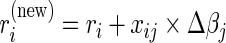 for all i. More critically, however, large-scale data sets often consist of many indicator variables resulting in
  that are sparse, such that
  for the majority of vector components j. We implement specialized, column-wise data structures to handle such sparse indicators that result in both significant reduction in memory requirements and enhanced performance under cyclic coordinate descent when compared with other traditional implementations. Further, Suchard and others (2013) describe how to translate this sparsity all the way through to computing the subject-specific gradient and Hessian contributions for a conditional Poisson regression model. While these contributions take a similar form to the terms indexed by i in (4.5) and (4.6), they do significantly differ. Under the Cox proportional hazards model, we must track and update the series of cumulative sums introduced through the growing risk sets
  for each subject i. Updating these prefix scans is costly, so we exploit the data sparsity by entering into this operation only if at least one observation in
  has a non-zero covariate along dimension j and embarking on the scan at the first non-zero entry instead of the beginning.
Finally, similar to Genkin and others (2007), our method employs a trust region approach in which we threshold the allowable update step size for each component so that parameter updates stay within the region where the quadratic function used in the Newton step remains a reasonable approximation to the objective function. We also note that, similar to Genkin and others (2007), instead of iteratively updating each variable until convergence, we take a single step in the direction of the negative gradient before proceeding on to the next variable. Because the optimal values of the other variables are themselves changing, tuning a particular variable to very high precision in each pass of the algorithm is not necessary.
5. Experiments
We test our algorithm on two different real data sets. Below, we briefly describe the data sets and also motivate their choice for our work.
5.1. Pediatric trauma
Injuries contribute to more deaths among children and adolescents that all other causes combined (National Center for Injury Prevention and Control, 2006). Accurate prediction of the outcome of pediatric trauma patients based on features present at the time of injury is essential for appropriate allocation of resources upon patient arrival to the hospital as well as predicting their final outcome. The goal of this portion of our work is to develop a model for predicting mortality after pediatric injury. Previous work in this area has mainly used LD analysis, with the number of predictors typically <20 (Mackersie, 2006; Resources for Optimal Care of the Injured Patient, 2006). While models utilizing a small number of predictors can be implemented in most standard statistical packages, the increase of dimensionality may lead to a decline in predictive and computational performance.
We obtain our data set from the National Trauma Data Bank, a trauma database maintained by the American College of Surgeons. The data set includes 210 555 patient records of injured children <15 years old collected over 5 years (2006–2010). We divide these data into a training data set (153 402 patients for 2006–2009) and a testing data set (57 153 patients for 2010). The mortality rate of the training set is 1.68% while that of the test set is 1.44%. There are a total of 125 952 binary predictors indicating the presence or absence of a particular attribute (or interaction among various attributes). We train our HD model using all the 125 952 predictors, while the LD model examines only 41 predictors. Table 1 summarizes various predictors used within both the HD and LD models.
Table 1.
Description of the predictors used for LD and HD models for pediatric trauma data
| Predictor type | # Predictors | Description | LD | HD |
|---|---|---|---|---|
| Main effects | ||||
| ICD-9 codes | 1890 | International classification of disease, Ninth revision | ✗ | ✓ |
| AIS codes (predots) | 349 | Abbreviated injury scale codes that includes body region, anatomic structure associated with the injury, and the level of injury | ✗ | ✓ |
| Interactions/combinations | ||||
| ICD-9, ICD-9 | 102 284 | Co-occurrences of two ICD-9 codes | ✗ | ✓ |
| AIS code, AIS code | 20 809 | Co-occurrences of two AIS codes | ✗ | ✓ |
| Body region, AIS score | 41 | Combinations of any of the nine body regions with the injury severity score (between 1 and 6) determined according to the AIS coding scheme | ✓ | ✓ |
| [Body region, AIS score], [Body region, AIS score] | 579 | Co-occurrences of two [body region, AIS score] combinations | ✗ | ✓ |
05.2. Breast cancer gene expression
In this experiment, we analyze a well-known breast cancer gene expression data set (van’t Veer and others, 2002). This data set is publicly available and consists of cDNA expression profiles of 295 tumor samples from patients diagnosed with breast cancer between 1984 and 1995 at the Netherlands Cancer Institute. Overall, 79 (26.78%) patients died during the follow-up time and the remaining 216 are censored. The total number of predictors (number of genes) is 24 885 each of which represents the log-ratio of the intensities of the two color dyes used for a specific gene. We train the HD model using all of the 24 885 predictors. For the LD model, we use the R glmpath (coxpath) package of Park and Hastie (2007) to generate the entire regularized paths and rank predictors in the order of their relative importance. We pick the top five predictors from the rank list and train an LD model on these for comparison. We randomly split the data into training (67%) and testing (33%) sets such that the mortality rate in both sets is approximately equal to the combined rate. We note that although this is not an HDMSS data set, analyzing gene expression data sets under a survival analysis framework is an important application area with considerable research interest.
5.3. Regularization parameter selection
To place the regularization parameters from the L1 and L2 penalities on the same scale, we reparameterize via  and
and  , respectively, for all j. We then select their regularization parameters τ and γ using a 4-fold cross validation on the training data. To accomplish this, we vary
  between 10−3 and 106 by multiples of 10 and select the value that returns the highest penalized partial likelihood averaged over the held-out validation sets.
5.4. Performance evaluation
The performance of fitted time-to-event models can be evaluated by assessing the quality of discrimination and calibration they provide. Similar to other regression models, the log-partial likelihood of the test data is a standard choice for comparing the discriminative power of various survival models. Among the approaches that also take censoring into account, Harrell's c-statistic (Harrell and others, 1982, 1996), which is an extension of the usual area under the receiver–operator characteristics curve (AUC), has become a popular choice among researchers (Chambless and others, 2011). To evaluate calibration of a model for survival data, we use an overall goodness-of-fit test proposed in Grønnesby and Borgan (1996). This test is an extension of the goodness-of-fit test for logistic regression models originally proposed by Hosmer and Lemeshow (1980). We briefly describe these two metrics below.
5.4.1. Harrell's c-statistic
Using this approach, we perform model discrimination by comparing the estimated and observed ordering of risk scores between pairs of comparable subjects. Two subjects  are comparable if at least one of the subjects in the pair develops the event (e.g. death) and the follow-up time duration for that subject is less than that of the other, i.e.
  and
and  . Further, a pair of comparable subjects
  is also concordant if the estimated risk of the subject who develops the event first is more than that of the other subject, i.e.
  ,
,  and
and  , where
  and
and  are the relative risk scores of the ith and jth subjects. Given a test set of n subjects, the c-statistic is written as
 |
(5.1) |
where  and
and  are the total number of comparable and concordant pairs, respectively.
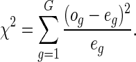
5.4.2. Hosmer–Lemeshow statistic
To estimate the overall goodness of fit using this test, we sort the subjects in the order of their increasing relative risk scores ( ) and then divide them into G equal-sized groups. For the gth group, the number of non-censored observations gives the observed number of events
  , while the number of expected events
  is equal to the sum of cumulative hazards (3.2) of all the subjects in that group. Note that, we use Breslow's estimator (Breslow, 1972) for computing the baseline hazard. The
  statistic for the overall goodness of fit is given by
 |
(5.2) |
6. Results
We now compare the performance of the LD and HD Cox models on both data sets. The goal of these experiments is to examine whether the HD Cox models made possible by our software deliver predictive advantages over their lower-dimensional counterparts.
6.1. Pediatric trauma data
Table 2 summarizes the results of our LD and HD models under both the L1 and L2 penalties for the pediatric trauma example. Note that under the L2 penalty, the estimate for any  is never exactly zero and thus all variables contribute to the final model. For this case, the number of predictors “selected” refers to the number of significant predictors
  . Although this threshold is arbitrary, it still provides a crude idea about the model complexity. Also, in the table, we compute the Hosmer–Lameshow
  statistic using
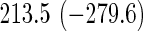
  . While the HD models for both the penalties have noticeably better discriminative power (log-likelihood, c-statistic) than the corresponding LD models, the LD models are better calibrated.
Table 2.
Comparison of LD and HD models for pediatric trauma data with L2 (top) and L1 (bottom) penalties
| Predictors |
|||||
|---|---|---|---|---|---|
| Model type | Overall | Selected | Log-likelihood | c-Statistic |  |
| Cox | |||||
| LD | 41 | 41 | −6952.07 | 0.90 | 148.32 |
| HD | 125 952 | 90 373 | −6709.96 | 0.94 | 190.82 |
| Exponential | |||||
| LD | 41 | 41 | −4270.01 | 0.88 | 124.39 |
| HD | 125 952 | 101 733 | −4372.41 | 0.94 | 543.28 |
| Weibull | |||||
| LD | 41 | 41 | −4242.38 | 0.88 | 131.60 |
| HD | 125 952 | 101 794 | −4557.10 | 0.94 | 749.22 |
| Log-logistic | |||||
| LD | 41 | 41 | −4120.66 | 0.89 | 95.37 |
| HD | 125 952 | 100 889 | −3765.45 | 0.94 | 95.02 |
| Log-normal | |||||
| LD | 41 | 41 | −3234.00 | 0.89 | 76.95 |
| HD | 125 952 | 88 244 | −3129.02 | 0.93 | 165.68 |
| Cox | |||||
| LD | 41 | 38 | −6952.02 | 0.90 | 143.73 |
| HD | 125 952 | 678 | −6673.58 | 0.94 | 163.74 |
| Exponential | |||||
| LD | 41 | 41 | −4271.23 | 0.88 | 122.58 |
| HD | 125 952 | 153 | −4034.67 | 0.92 | 94.34 |
| Weibull | |||||
| LD | 41 | 41 | −4243.57 | 0.88 | 126.84 |
| HD | 125 952 | 151 | −3997.28 | 0.92 | 107.99 |
| Log-logistic | |||||
| LD | 41 | 41 | −4122.07 | 0.89 | 94.73 |
| HD | 125 952 | 432 | −3777.83 | 0.94 | 83.00 |
| Log-normal | |||||
| LD | 41 | 41 | −3236.79 | 0.89 | 80.71 |
| HD | 125 952 | 168 | −2974.49 | 0.93 | 89.36 |
For L2 penalization, the number of selected predictors refers to the number of significant predictors  . In both cases, bold emphases represent superior performance of one type of Cox model over the other. For a more comprehensive comparison, the results obtained using four parametric models (Mittal and others, 2013) are also presented in the lower parts of the table.
To gain more understanding about the performance of Cox models, Table 2 also compares their respective predictive performance with that of four parametric survival models. These results are taken from our recent work on large-scale regularized parametric survival models (Mittal and others, 2013). Note that, in the interest of the context of this paper, bold emphasis is only used to highlight the superior performance of one kind of Cox model over the other. Also note that since the log-likelihood for Cox and parametric models are formulated differently, they are not directly comparable. The c-statistics and  statistics demonstrate that some parametric models provide similar discriminative performance when compared with the Cox models while being better calibrated. Moreover, in the case of L1 penalization, all parametric models use a fewer number of predictors when compared with the Cox models. Both these observations indicate slight overfitting of Cox models to the data when compared with their parametric counterparts. Readers are also encouraged to refer to supplementary material available at Biostatistics online for an additional experiment on the predictive performance of Cox models.
6.2. Breast cancer gene expression data
Table 3 shows the results of the gene expression example for LD and HD models using L1 and L2 penalties. In this case, we compute the Hosmer–Lameshow  statistic using just
  due to the smaller size of the test data set. While the discriminative performance of both the methods is similar for both types of penalization, the HD model is better calibrated. The case of L1 penalization is particularly interesting since, in this case, the HD model is four times better calibrated than the LD model using only 20 predictors. Also, significantly better calibration of this model compared with the HD L2 penalized one (that uses almost all predictors) suggests model overfitting in the latter case. Like the previous example, the corresponding results of four types of regularized parametric models are also presented for comparison.
Table 3.
Comparison of LD and HD models for gene expression data with L2 (top) and L1 (bottom) penalties
| Predictors |
|||||
|---|---|---|---|---|---|
| Model type | Overall | Selected | Log-likelihood | c-Statistic |  |
| Cox | |||||
| LD | 5 | 5 | −71.13 | 0.71 | 26.35 |
| HD | 24 496 | 24 026 | −72.10 | 0.76 | 12.75 |
| Exponential | |||||
| LD | 5 | 5 | −86.26 | 0.71 | 16.83 |
| HD | 24 496 | 24 344 | −98.72 | 0.75 | 112.69 |
| Weibull | |||||
| LD | 5 | 5 | −85.64 | 0.71 | 12.79 |
| HD | 24 496 | 22 299 | −85.56 | 0.70 | 9.34 |
| Log-logistic | |||||
| LD | 5 | 5 | −85.65 | 0.70 | 14.74 |
| HD | 24 496 | 22 090 | −86.14 | 0.70 | 5.37 |
| Log-normal | |||||
| LD | 5 | 5 | −52.10 | 0.70 | 16.02 |
| HD | 24 496 | 24 154 | −65.14 | 0.66 | 23.61 |
| Cox | |||||
| LD | 5 | 4 | −71.10 | 0.71 | 30.19 |
| HD | 24 496 | 20 | −72.64 | 0.71 | 7.49 |
| Exponential | |||||
| LD | 5 | 5 | −86.27 | 0.71 | 17.14 |
| HD | 24 496 | 13 | −87.51 | 0.67 | 2.74 |
| Weibull | |||||
| LD | 5 | 5 | −85.63 | 0.71 | 12.79 |
| HD | 24 496 | 13 | −86.80 | 0.66 | 3.75 |
| Log-logistic | |||||
| LD | 5 | 5 | −85.65 | 0.70 | 14.71 |
| HD | 24 496 | 9 | −86.20 | 0.68 | 3.66 |
| Log-normal | |||||
| LD | 5 | 5 | −52.10 | 0.70 | 15.98 |
| HD | 24 496 | 9 | −53.46 | 0.66 | 8.57 |
For L2 penalization, the number of selected predictors refers to the number of significant predictors  . In both cases, bold emphases represent superior performance of one type of Cox model over the other. For a more comprehensive comparison, the results obtained using four parametric models (Mittal and others, 2013) are also presented in the lower parts of the table.
7. Computation time
Table 4 reports the time taken for fitting Cox models for the optimum value of the regularization parameter (found using 4-fold cross-validation as described in Section 5.3) to the two sets of LD and HD data sets. We perform all of these experiments on a system with an Intel 2.4 GHz processor and 8 GB of memory. Even though the time taken to fit HD models to the pediatric trauma data set is much greater than that taken to fit LD models, given the scale of the problem (153 402 patients with 125 952 predictors), the performance of the method may be acceptable in many applications. For the sake of completion, we also present the corresponding computation times of the four parametric models (Mittal and others, 2013).
Table 4.
Computation time (in seconds) taken for training LD and HD models using L2 and L1 penalties for pediatric trauma (top) and gene expression (bottom) data sets
| L2 |
L1 |
|||
|---|---|---|---|---|
| Model type | LD | HD | LD | HD |
| Cox | 0.28 | 525.12 | 0.27 | 498.37 |
| Exponential | 1.00 | 4453.00 | 1.00 | 2588.00 |
| Weibull | 3.00 | 3406.00 | 2.00 | 2600.00 |
| Log-logistic | 2.00 | 2794.00 | 2.00 | 3278.00 |
| Log-normal | 6.00 | 3250.00 | 6.00 | 3101.00 |
| Cox | 0.01 | 0.80 | 0.01 | 0.59 |
| Exponential | 1.00 | 4.00 | 1.00 | 8.00 |
| Weibull | 1.00 | 12.00 | 1.00 | 30.00 |
| Log-logistic | 1.00 | 13.00 | 1.00 | 38.00 |
| Log-normal | 1.00 | 51.00 | 1.00 | 52.00 |
For a more comprehensive comparison, the run-times of four parametric models (Mittal and others, 2013) are also presented.
We also provide detailed comparisons between the performance of our method with that of the coxnet method (Simon and others, 2011). For the first set of comparisons, like our method, coxnet was also subjected to a 4-fold cross-validation over the training sets using a fixed set of regularization values (i.e.  varied between 10−3 and 109 by multiples of 10). For a fair comparison, we adjusted the convergence threshold of our method such that both the methods always returned similar log-partial likelihood values at convergence. Table 5 shows the run-times in seconds for both methods on an LD pediatric trauma data set (large n and small p) and HD gene expression data set (small n and large p). The corresponding log-partial likelihood values obtained at convergence are in parentheses.
Table 5.
Comparison of computation times (in seconds) taken for training coxnet and our method
| LD pediatric trauma |
HD gene expression |
|||
|---|---|---|---|---|
| Model type | L2 | L1 | L2 | L1 |
| coxnet |  |
 |
 |
 |
| Our method |  |
 |
 |
 |
| coxnet |  |
 |
 |
 |
| Our method |  |
 |
 |
 |
Top: the cross-validation for both the methods was performed by varying the hyperparameter value between 10−3 and 109 by multiples of 10. Bottom: the cross-validation for both the methods was performed over the regularization path chosen by coxnet. The corresponding penalized log-likelihood achieved at convergence are in parentheses. Bold emphases represent superior performance of one method over the other.
It is known that coxnet's performance is most optimized for fitting the entire regularization path automatically chosen by the algorithm. To this end, we also subjected our method to cross-validation over the regularization path chosen by coxnet. For an LD pediatric trauma data set with L1 penalty, the regularization path selected by coxnet consisted of 65 different values. For all other settings, the path length was 100. Table 5 shows the corresponding results.
Similar run-time comparisons for an LD gene expression data set were intentionally skipped due to the very small size of the training data ( ). More importantly, we were not able to load the HD pediatric trauma data set (
 ) into coxnet since it does not support sparse matrix formats for the input data.
8. Conclusions
We present a tool to perform regularized Cox survival analysis on HDMSS data. Through our experiments, we demonstrate that, with the advantage of fitting directly on HDMSS data, we can obtain models that have better predictive accuracy and calibration. We provide a freely available software tool that implements our proposed algorithm. This tool is a part of our HD, regularized, generalized linear models library that can also utilize inexpensive, massively parallel devices known as graphics processing units (Suchard and others, 2013). These devices can provide more than an order-of-magnitude speed-up and in principle could be easily applied for the work presented in this paper. Bayesian extensions to our current work could explore the hierarchical framework to simultaneously model multiple time-to-event endpoints and also model multi-level structure such as patients nested within hospitals. Owing to their competitive performance, we also plan to extend our current work to more efficient implementation of parametric models than the one that currently exists (Mittal and others, 2013).
9. Software
We have publicly released the C++ implementation of our algorithm. This code is a part of our software for HD, regularized, generalized linear models (Suchard and others, 2013). The code can be downloaded from http://bsccs.googlecode.com. Computation of various evaluation measures discussed in Section 5 is also integrated into the code.
Supplementary material
Supplementary material is available at http://biostatistics.oxfordjournals.org.
Funding
The research reported in this publication was supported by the National Institute for General Medical Sciences of the National Institutes of Health under award number R01GM087600 and by the National Science Foundation under award number IIS-1251151.
Supplementary Material
Acknowledgements
Conflict of Interest: None declared.
References
- Box-Steffensmeier J. M., Jones B. S. Event History Modeling: A Guide for Social Scientists. Cambridge, UK: Cambridge University Press; 2004. [Google Scholar]
- Breslow N. Discussion on Regression models and life tables by D. R. Cox. Journal of the Royal Statistical Society Series B. 1972;34:216–217. [Google Scholar]
- Chambless L. E., Cummiskey C. P., Cui G. Several methods to assess improvement in risk prediction models: extension to survival analysis. Statistics in Medicine. 2011;30(1):22–38. doi: 10.1002/sim.4026. [DOI] [PubMed] [Google Scholar]
- Collett D. Modelling Survival Data for Medical Research. 2nd edition. London, UK: Chapman-Hall; 2003. [Google Scholar]
- Cox D. R. Regression models and life-tables. Journal of the Royal Statistical Society. Series B (Methodological) 1972;34(2):187–220. [Google Scholar]
- Engler D., Li Y. Survival analysis with high-dimensional covariates: an application in microarray studies. Statistical Applications in Genetics and Molecular Biology. 2009;8(1):1–22. doi: 10.2202/1544-6115.1423. [DOI] [PMC free article] [PubMed] [Google Scholar]
- Evers L., Messow C.-M. Sparse kernel methods for high-dimensional survival data. Bioinformatics. 2008;24(14):1632–1638. doi: 10.1093/bioinformatics/btn253. [DOI] [PubMed] [Google Scholar]
- Friedman J., Hastie T., Tibshirani R. Regularization paths for generalized linear models via coordinate descent. Journal of Statistical Software. 2010;33(1):1–22. [PMC free article] [PubMed] [Google Scholar]
- Genkin A., Lewis D. D., Madigan D. Large-scale Bayesian logistic regression for text categorization. Technometrics. 2007;49(3):291–304. [Google Scholar]
- Goeman J. J. L1 penalized estimation in the Cox proportional hazards model. Biometrical Journal. 2010;52(1):70–84. doi: 10.1002/bimj.200900028. [DOI] [PubMed] [Google Scholar]
- Gorst-Rasmussen A., Scheike T. H. Coordinate descent methods for the penalized semiparametric additive hazards model. Journal of Statistical Software. 2012;47:9. [Google Scholar]
- Grønnesby J. K., Borgan Ø. A method for checking regression models in survival analysis based on the risk score. Lifetime Data Analysis. 1996;2(4):315–328. doi: 10.1007/BF00127305. [DOI] [PubMed] [Google Scholar]
- Harrell F. E., Califf R. M., Pryor D. B., Lee K. L., Rosati R. A. Evaluating the yield of medical tests. Journal of the American Medical Association. 1982;247(18):2543–2546. [PubMed] [Google Scholar]
- Harrell F. E, Lee K. L., Mark D. B. Multivariable prognostic models: issues in developing models, evaluating assumptions and adequacy, and measuring and reducing errors. Statistics in Medicine. 1996;15(4):361–387. doi: 10.1002/(SICI)1097-0258(19960229)15:4<361::AID-SIM168>3.0.CO;2-4. [DOI] [PubMed] [Google Scholar]
- Heckman J. J., Singer B. Longitudinal Analysis of Labor Market Data. Cambridge, UK: Cambridge University Press; 1985. [Google Scholar]
- Hoerl A. E., Kennard R. W. Ridge regression: biased estimation for nonorthogonal problems. Technometrics. 1970;12:55–67. [Google Scholar]
- Hosmer D. W., Lemeshow S. Goodness of fit tests for the multiple logistic regression model. Communications in Statistics - Theory and Methods. 1980;9(10):1043–1069. [Google Scholar]
- Hosmer D. W., Lemeshow S., May S. Applied Survival Analysis: Regression Modeling of Time to Event Data (Wiley Series in Probability and Statistics) 2nd edition. Wiley-Interscience; 2008. [Google Scholar]
- Ishwaran H., Kogalur U. B., Chen X., Minn A. J. Random survival forests for high-dimensional data. Statistical Analysis and Data Mining. 2011;4(1):115–132. [Google Scholar]
- Ishwaran H., Kogalur U. B., Gorodeski E. Z., Minn A. J., Lauer M. S. High-dimensional variable selection for survival data. Journal of the American Statistical Association. 2010;105(489):205–217. [Google Scholar]
- Kalbfleisch J. D., Prentice R. L. The Statistical Analysis of Failure Time Data. New York: John Wiley and Sons; 1980. [Google Scholar]
- Kivinen J., Warmuth M. K. Relative loss bounds for multidimensional regression problems. Machine Learning. 2001:301–329. . Norwell, MA:Kluwer Academic Publishers. [Google Scholar]
- Klein J. P., Moeschberger M. L. Survival Analysis: Techniques For Censored and Truncated Data. 2nd edition. New York: John Willey and Sons; 2003. [Google Scholar]
- Koh K., Kim S.-J., Boyd S. An interior-point method for large-scale L1-regularized logistic regression. Journal of Machine Learning Research. 2007;8:1519–1555. [Google Scholar]
- Mackersie R. C. History of trauma field triage development and the American College of Surgeons criteria. Prehospital Emergency Care. 2006;10(3):287–294. doi: 10.1080/10903120600721636. [DOI] [PubMed] [Google Scholar]
- Mittal S., Madigan D., Cheng J. Q., Burd R. S. Large-scale Bayesian parametric survival analysis. Statistics in Medicine. 2013 doi: 10.1002/sim.5817. ( doi:10.1002/sim.5817.) [DOI] [PMC free article] [PubMed] [Google Scholar]
- National Center for Injury Prevention and Control. CDC Injury Fact Book. Atlanta, GA: Centers for Disease Control and Prevention; 2006. [Google Scholar]
- Oakes D. Biometrika centenary: survival analysis. Biometrika. 2001;88(1):99–142. [Google Scholar]
- Park M. Y., Hastie T. L1-regularization path algorithm for generalized linear models. Journal of the Royal Statistical Society. 2007;69(4):659–677. [Google Scholar]
- Resources for Optimal Care of the Injured Patient. Committee on Trauma. Chicago, IL: American College of Surgeons; 2006. [Google Scholar]
- Shivaswamy P. K., Chu W., Jansche M. IEEE International Conference on Data Mining. Omaha: NE; 2007. A support vector approach to censored targets; pp. 655–660. [Google Scholar]
- Simon N., Friedman J., Hastie T., Tibshirani R. Regularization paths for Cox's proportional hazards model via coordinate descent. Journal of Statistical Software. 2011;39(5):1–13. doi: 10.18637/jss.v039.i05. [DOI] [PMC free article] [PubMed] [Google Scholar]
- Sohn I., Kim J., Jung S.-H., Park C. Gradient lasso for Cox proportional hazards model. Bioinformatics. 2009;25(14):1775–1781. doi: 10.1093/bioinformatics/btp322. [DOI] [PubMed] [Google Scholar]
- Suchard M. A., Simpson S. E., Zorych I., Ryan P., Madigan D. Massive parallelization of serial inference algorithms for generalized linear models. ACM Transactions on Modeling and Computer Simulation. 2013;23:10. doi: 10.1145/2414416.2414791. [DOI] [PMC free article] [PubMed] [Google Scholar]
- Tibshirani R. Regression shrinkage and selection via the lasso. Journal of the Royal Statistical Society (Series B) 1996;58:267–288. [Google Scholar]
- Tibshirani R., Hastie T., Friedman J. H. Regularization paths for generalized linear models via coordinate descent. Journal of Statistical Software. 2010;33:1. [PMC free article] [PubMed] [Google Scholar]
- Tseng P. Convergence of a block coordinate descent method for nondifferentiable minimization. Journal of Optimization Theory and Applications. 2001;109(3):475–494. [Google Scholar]
- Van Belle V., Pelckmans K., Van Huffel S., Suykens J. A. K. Improved performance on high-dimensional survival data by application of survival-SVM. Bioinformatics. 2011;27(1):87–94. doi: 10.1093/bioinformatics/btq617. [DOI] [PubMed] [Google Scholar]
- van't Veer L. J., Dai H., van de Vijver M. J., He Y. D., Hart A. A., Mao M., Peterse H. L., van der Kooy K., Marton M. J., Witteveen A. T. Gene expression profiling predicts clinical outcome of breast cancer. Nature. 2002;415(6871):530–536. doi: 10.1038/415530a. and others. [DOI] [PubMed] [Google Scholar]
- Witten D. M., Tibshirani R. Survival analysis with high-dimensional covariates. Statistical Methods in Medical Research. 2010;19(1):29–51. doi: 10.1177/0962280209105024. [DOI] [PMC free article] [PubMed] [Google Scholar]
- Wu T. T., Lange K. Coordinate descent algorithms for lasso penalized regression. The Annals of Applied Statistics. 2008;2(1):224–244. doi: 10.1214/10-AOAS388. [DOI] [PMC free article] [PubMed] [Google Scholar]
- Yang Y., Zou H. A cocktail algorithm for solving the elastic net penalized Cox's regression in high dimensions. Statistics and its Interface. 2012;6(2):167–173. [Google Scholar]
- Zhang T., Oles F. J. Text categorization based on regularized linear classification methods. Information Retrieval. 2000;4:5–31. [Google Scholar]
Associated Data
This section collects any data citations, data availability statements, or supplementary materials included in this article.