

Abstract
For designing, monitoring, and analyzing a longitudinal study with an event time as the outcome variable, the restricted mean event time (RMET) is an easily interpretable, clinically meaningful summary of the survival function in the presence of censoring. The RMET is the average of all potential event times measured up to a time point τ and can be estimated consistently by the area under the Kaplan–Meier curve over  . In this paper, we study a class of regression models, which directly relates the RMET to its “baseline” covariates for predicting the future subjects’ RMETs. Since the standard Cox and the accelerated failure time models can also be used for estimating such RMETs, we utilize a cross-validation procedure to select the “best” among all the working models considered in the model building and evaluation process. Lastly, we draw inferences for the predicted RMETs to assess the performance of the final selected model using an independent data set or a “hold-out” sample from the original data set. All the proposals are illustrated with the data from the an HIV clinical trial conducted by the AIDS Clinical Trials Group and the primary biliary cirrhosis study conducted by the Mayo Clinic.
Keywords: Accelerated failure time model, Cox model, Cross-validation, Hold-out sample, Personalized medicine, Perturbation-resampling method
1. Introduction
For a longitudinal study with time T to a specific event as the primary outcome variable, commonly used summary measures for the distribution of T are the mean, median, or t-year event rate. Due to potential censoring for T, the mean may not be estimable. If the censoring is heavy, the median cannot be empirically identified either. The t-year survival rate can be estimated at a specific time t, but this estimate may not be suitable for summarizing the global profile of T over the duration of the study. On the other hand, based on the design of the study and clinical considerations, one may pre-specify a time point τ and utilize the expected value μ of  , the so-called restricted mean event time (RMET), as a summary parameter. This parameter is the mean of T for all potential study patients followed up to time τ, which has heuristic and clinically meaningful interpretation (Chen and Tsiatis, 2001; Andersen and others, 2004; Royston and Parmar, 2011; Zhao and others, 2012). Moreover, this model-free parameter can be estimated consistently via the standard Kaplan–Meier (KM) curve, that is, the area under the curve up to τ. Inference procedures for the RMET with censored event-time observations were extensively studied by Zhao and Tsiatis (1997; 1999) under a more general setting.
In order to compare two groups, say, A and B, with censored event-time observations, practitioners routinely use the hazard ratio to quantify the group difference. Note that for this between-group contrast measure, there is no “background” rate one can utilize to evaluate whether such a hazard ratio estimate represents a clinically meaningful difference, information which is necessary for the purposes of risk–benefit decision making. Furthermore, when the proportional hazards assumption is not valid, the standard maximum partial likelihood estimator of the hazard ratio approximates a parameter which is difficult, if not impossible, to interpret as the treatment contrast (Lin and Wei, 1989; Rudser and others, 2012). Moreover, this parameter depends, oddly, on the nuisance, study-specific censoring distributions (Lin and Wei, 1989). It follows that the hazard ratio estimators at the interim and final analyses from the same study or estimators from independent studies with an identical study populations would estimate different, uninterpretable parameters due to differential follow-up patterns. Therefore, it is highly desirable to consider an estimable, model-free, and censoring-independent parameter to quantify the treatment difference for coherent and consistent assessments between interim and final analyses within a study, as well as across independent studies.
Model-free parameters for the treatment difference can be constructed via two RMETs, say,  and
and  . As an example, to evaluate the added value of a potent protease inhibitor, indinavir, for HIV patients, a pivotal study ACTG 320 was conducted by the AIDS Clinical Trials Group (ACTG). This randomized, double-blind study (Hammer and others, 1997) compared a three-drug combination, indinavir, zidovudine, and lamivudine, with the standard two-drug combination, zidovudine and lamivudine. There were 1156 enrolled for the study. One of the endpoints was the time to AIDS or death with a follow-up time of about 1 year for each patient. Figure 1 presents the KM curves for these two treatment groups. The hazard ratio estimate is 0.50 and the corresponding 0.95 confidence interval is (0.33, 0.76) with a p-value of 0.001. With
  days, the estimated RMET was 277 days for the control and was 288 days for the three-drug combination. The estimated difference with respect to the RMET is 11 days with the corresponding 0.95 confidence interval of
  and a p-value of 0.005. Although the treatment efficacy for the three-drug combination is highly statistically significant, its clinical benefit is debatable using this metric of the absolute difference with respect to the RMET. If we mimic the concept of the hazard ratio or relative risk as a summary measure for the treatment contrast, one may consider a model-free ratio R of
  and
and  , where
  and
and  are the RMETs for arms A and B, respectively. With the above HIV data, if B is the treatment group receiving the three-drug combination, the estimated R is 0.55 with a p-value of
  also an impressive statistically significant result. For a single arm,
  is the average of the years lost from the healthy state up to
  a meaningful alternative to μ as a summary parameter for the distribution of T. Note that either using the absolute difference or the ratio to quantify the group-contrast via the RMET, there is a background value from the control arm for assessing the added value of indinavir for treating HIV patients from clinical benefit–risk–cost perspectives.
Fig. 1.
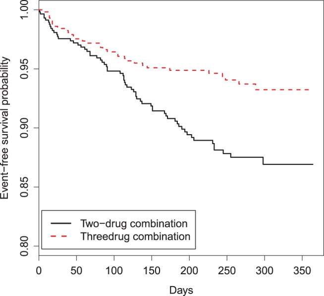
KM estimates of the survival functions of the two randomized groups based on the ACTG 320 data.
In this paper, we are interested in building prediction models for the RMET with the subject's “baseline” covariates and make inferences of such predictions. Existing regression models, such as the Cox model, can be candidates to create such a “personalized” prediction scheme. However, it seems more natural to model the RMET with the covariates directly, not via the hazard function (Andersen and others, 2004). In this article, we consider a class of models which takes this approach and study the properties of the corresponding inference procedures. Since it is unlikely that any model will be precisely correct, our ultimate goal is to choose the best “fitted” model among a set of candidate working models to stratify the future patients. To avoid overly optimistic results, we randomly split the data set into two pieces. Using the first piece, called the training-evaluation set, we utilize a cross-validation (CV) procedure to build and select the final model. We then use the second data set, called the hold-out set, to make inferences about the RMETs over a range of scores created from the final selected model. This final step is crucial to have a valid assessment of the performance of the proposed prediction procedure. We use a data set from a well-known clinical study conducted at Mayo Clinic (Therneau and Grambsch, 2000) for treating a liver disease to illustrate the proposals.
2. Regression models for RMET
For a typical subject with event time T, let Z be the corresponding q-dimensional baseline covariate vector. Suppose that T is subject to right censoring by a random variable C, which is assumed to be independent of T and Z. The observable quantities are  , where
  ,
,  , and
, and  is the indicator function. The data,
  , consist of
  independent copies of
  . Suppose that for a time point
 . The restricted survival time
  may also be censored, but its expected value μ is estimable. Let
  be the corresponding Y for the
  th subject,
  . A natural estimator for μ is
  where
where  is the KM estimator for the survival function of T based on
  . The inference procedures for μ have been extensively studies, for example, by Zhao and Tsiatis (1997; 1999) and Zhao and others (2012).
Now, let  . It follows from Andersen and others (2004), one may model this directly with Z:
 |
(2.1) |
where  is a given smooth and strictly increasing link function,
  is a
is a  -dimension unknown vector and
  . The link function can be the identity function. On the other hand, since the support of the restricted event time Y is finite, it may be appropriate to consider
  being an increasing function mapping
  to the real line. A special link function is
  which mimics the logistic regression. Note that with this specific link, for the two-sample problem, the regression coefficient of the treatment indicator is
 |
an odds-ratio like summary for the group contrast.
For the general link function  following the least squares principle, an inverse probability censoring weighted estimating function of
  is
is
 |
where  and
and  is the KM estimator of the censoring time C based on
  . Let
. Let  be the unique root of
  . In Appendix A of supplementary material available at Biostatistics online, we show that under mild regularity conditions,
  converges to a constant
  in probability, even when Model (1) is misspecified, an important property for building a prediction model. In addition, we show that as
 converges weakly to a mean zero Gaussian distribution. We also provide inference procedures for
  in Appendix A of supplementary material available at Biostatistics online. Note that Andersen and others (2004) studied Model (1) via a specific log-link
  using a pseudo-observation technique to make inferences about the regression coefficient. However, there is no systematic procedure in the literature for evaluating the adequacy of such a working model from the prediction point of view.
Using the above model, one may estimate  by
by  , for any fixed
  where
where  . The distribution of
  can be approximated by the delta method. Note that
  can also be estimated via, for example, a Cox model (Cox, 1972). Specifically, let the hazard function for given z be
  where
where  is a q-dimensional unknown vector and
  is the nuisance baseline hazard function. It follows that
  can be estimated by
 |
where  and
and  are the maximum partial likelihood estimator for
  and the Breslow estimator for
  respectively.
Alternatively, one may use the accelerated failure time (AFT) model (Kalbfleisch and Prentice, 2002),  to make inference about
  , where
  is a q-dimensional unknown vector and
  is the error term whose distribution is entirely unspecified. Here,
  can be estimated via a rank-based estimating function (Tsiatis, 1990; Jin and others, 2003). Let
  be the corresponding estimator for
  . One may estimate the survival function of
  by KM estimator based on the data
  . Let the resulting estimator be denoted by
  . Then one can estimate
  by
by  . Note that when
 is estimable for any given covariate z. In practice, we can always set the censoring indicator at one for the observation with the largest
  in estimating the survival function of
  . Although these estimators for
  may be biased, and under general model misspecification, will depend on the censoring distribution, they may still produce reasonable predictions for the RMET. Note that the parameters in either Cox or AFT working model may be estimated with the entire observed data, not restricted by the follow-up information up to time point τ.
3. Model selection and evaluation
All the models for estimating  discussed in the previous section are approximations to the true model. To compare these models, one may compare the restricted event time Y with the covariate vector z and its predicted
  . A reasonable predicted error measure is
  where the expected value is with respect to the data and the future subject's
  . If there is no censoring, the empirical apparent prediction error is
  which is obtained by first using the entire data to compute
  and then using the same data to estimate the predicted error. To avoid bias, we utilize a CV procedure to estimate such a predicted error (Tian and others, 2007). Specifically, consider a class of models for
  . For each model, we randomly split the data set into K disjoint subsets of approximately equal sizes, denoted by
  . For each k, we use all observations which are not in
  to obtain a model-based prediction rule
  for Y, and then estimate the total absolute prediction error for observations in
  by
by
 |
Then we use the average  as a K-fold CV estimate for the absolute prediction error. We may repeat the aforementioned procedure a large number of, say
  times with different random partitions. Then the average of the resulting J cross-validated estimates is the final random K-fold CV estimate for the absolute prediction error of the fitted regression model. Generally, the model which yields the smallest cross-validated absolute prediction error estimate among all candidate models is chosen as the final model. On the other hand, a parsimonious model may be preferable if its empirical predicted error is comparable with a more complex “optimal” model. We then refit the entire training-evaluation data set with this selected model for making predictions based on
  .
.
Note that in the training stage of this CV process, a candidate model may be obtained via a complex variable selection process. For example, a Cox model may be built with a stepwise regression or lasso procedure. In this case, the final choice for creating the score would be refitting the entire training-evaluation data set with the selected model building algorithm.
4. Inference about subject-specific RMET
Ideally, one would use a model-free estimate of  for subject-specific prediction of RMET. However, a fully non-parametric estimate of
  is not feasible due to the curse of dimensionality. A practical way to create a prediction scheme using the baseline covariates is to utilize the “best” candidate among all the working models considered in the previous section to create a scoring system for the future subject's RMET. Then we use this univariate score to stratify subjects and make inferences about the stratum-specific RMET with a data set from an independent study or the hold-out sample from the same study.
To this end, let the estimated  from the final selected model be denoted by
  and for a future subject with
  let its prediction score be denoted by
  . That is, for each future subject, the covariate vector Z is reduced to a univariate V which is a function of Z. If the selected model is close to the true one, we expect that
  . In general, however, the group mean
  by clustering all subjects with Z, whose
  may be different from v. Therefore, the conventional parametric inferences about predicting
  via the selected model may not be valid. On the other hand, since we reduce the covariate information to a univariate score V, one may utilize a non-parametric estimation procedure to draw valid inferences about
  .
.
To make non-parametric inference about  simultaneously across a range of the score
  we use a fresh independent data set or “hold-out” set from the original data set. With slight abuse of notation, let such a fresh data set be denoted by
  . We propose to use local linear smoothing method to estimate
  non-parametrically. To this end, for a score v inside the support of V, let
  and
and  be the solution of the estimating equation
 |
where  is a smooth symmetric kernel function with a finite support,
 is the smoothing bandwidth,
 |
is the local non-parametric estimator for the survival function of C (Dabrowska, 1987; 1989) and  . Here,
  is a strictly increasing function from
  to the entire real line given a priori. The resulting local linear estimator for
  is
is  . As
. As  and
and  ,
,  converges weakly to a mean zero Gaussian. The details are given in Appendix B of supplementary material available at Biostatistics online. Since the censoring time C is assumed to be independent of
  generally the non-parametric KM estimator based on the entire sample is used in the inverse probability weighting method for
  . Here, we use the local estimator
  in above estimating equation. In Appendix B of supplementary material available at Biostatistics online, we show that this estimation procedure results in a more accurate estimator for
  than that using
  . Note that when the empirical distribution of
  is quite non-uniform, transforming the score via an appropriate function before smoothing could potentially improve the performance of the kernel estimation (Park and others, 1997; Cai and others, 2010).
The perturbation-resampling method proposed by Gilbert and others (2002) and Tian and others (2005) can be used to construct pointwise and simultaneous confidence intervals for  over v. To this end, let
  and
and  be the solution of the perturbed estimating equation
 |
where  are positive random variables with unit mean and variance and independent of the observed data, and
 |
Then a perturbed estimator for  is
is  . Conditional on the observed data, the limiting distribution of
  approximates the unconditional counterpart of
  . It follows that one can estimate the variance of
  by
by  the empirical variance of
  realized
  s using
  independent sets of
  . Based on generated
  one may construct
  confidence interval of
  as
as  where
where  is the upper 100
 percentage point of the standard normal. For an interval
  , a subset of the support of
  the
the  simultaneous confidence band of
  can be constructed similarly as
  where
where
 |
As with any non-parametric function estimation problem, it is crucial to choose an appropriate bandwidth h in order to make proper inference about  . In Appendix C of supplementary material available at Biostatistics online, we propose a CV procedure to choose an optimal h value which minimizes a weighted cross-validated absolute prediction error.
5. Example for subject-specific prediction
In this section, we use a well-known data set from a liver study to illustrate how to build and select a model, and make inferences simultaneously about the RMETs over a range of scores created by the final model. This liver disease study in primary biliary cirrhosis (PBC) was conducted between 1974 and 1984 to evaluate the drug D-penicillamine, which was found to be futile with respect to the patient's mortality. The investigators for the study then used this rich data set to build a prediction model with respect to mortality (Fleming and Harrington, 1991). There were a total of 418 patients involved in the study, including 112 patients who did not participate in the clinical trials, but had available baseline and mortality information. For illustration, any missing baseline value was imputed by the corresponding sample mean calculated from its observed counterparts in the study. We randomly split the data set with equal sizes as the training and hold-out sets.
For our analysis, we consider 16 baseline covariates: gender, histological stage of the disease (1, 2, 3, and 4), presence of ascites, edema, hepatomegaly or enlarged liver, blood vessel malformations in the skin, log-transformed age, serum albumin, alkaline phosphatase, aspartate aminotransferase, serum bilirubin, serum cholesterol, urine copper, platelet count, standardized blood clotting time, and triglycerides. Three models discussed in Section 2 with these covariates included additively were considered in the model selection. They are the Cox model, the AFT model, and the new RMET model. Moreover, since a more parsimonious Cox model using five of these covariates (edema, log-transformed age, bilirubin, albumin, and standardized blood clotting time) has been established as a prediction model in the literature (Fleming and Harrington, 1991), we also considered the aforementioned three types of models with these five covariates additively in our analysis. There are, therefore, six different models were considered. Note that there was no variable selection procedure involved in the model building stage for this illustration.
Figure 2 shows the KM curve for the patients’ survival, estimated using the entire data set. None of the patients’ follow-up times exceed 13 years. Since the tail part of the KM estimate is not stable. We let  years for illustration. The overall 10-year survival rate is about 44%. Table 1 presents the
  prediction error estimates for the RMET up to 10 years for the three model building procedures based on 100 random 5-fold CVs. With CV, the
  prediction error is minimized at 1.94 in years when the proposed regression Model (1) with the logistic link function
  based on five baseline covariates is utilized.
Fig. 2.
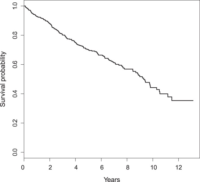
KM estimate of the overall patient survival function based on the PBC data.
Table 1.
 prediction error estimates for the RMET up to 10 years of the three model building procedures based on 100 random 5-fold CVs
 prediction error with CV prediction error with CV |
|||
|---|---|---|---|
| Cox model | AFT model | New model | |
| 5 covariates | 2.34 | 2.00 | 1.94 |
| 16 covariates | 2.34 | 2.11 | 2.10 |
The final model is obtained by fitting the RMET model with five covariates:
 |
We then use the score created by this model to make prediction and stratification for subjects in the hold-out set.
For predicting future restricted event time, we use the procedures proposed in Section 4 to estimate the subject-specific RMET  over a range of score v's, and the perturbation-resampling method with
  independent sets of
  from the unit exponential to construct its 0.95 pointwise and simultaneous confidence intervals over the interval
  in years, where 0.07 and 9.52 are the 2nd and 98th percentiles of observed scores in the hold-out set. Here, we let
  be the Epanechnikov kernel and the bandwidth be 2.1, as selected via CV discussed in Appendix C of supplementary material available at Biostatistics online. The results are presented in Figure 3(a). For comparison, we also present the corresponding results in Figure 3(b) with the survival function of the censoring time C being estimated based on the entire sample rather than locally as proposed in Section 4. As expected, the resulting estimator for
  is less accurate, e.g. the 95% confidence interval for
  is 24.8% wider when the survival function of C is estimated based on the entire sample.
Fig. 3.
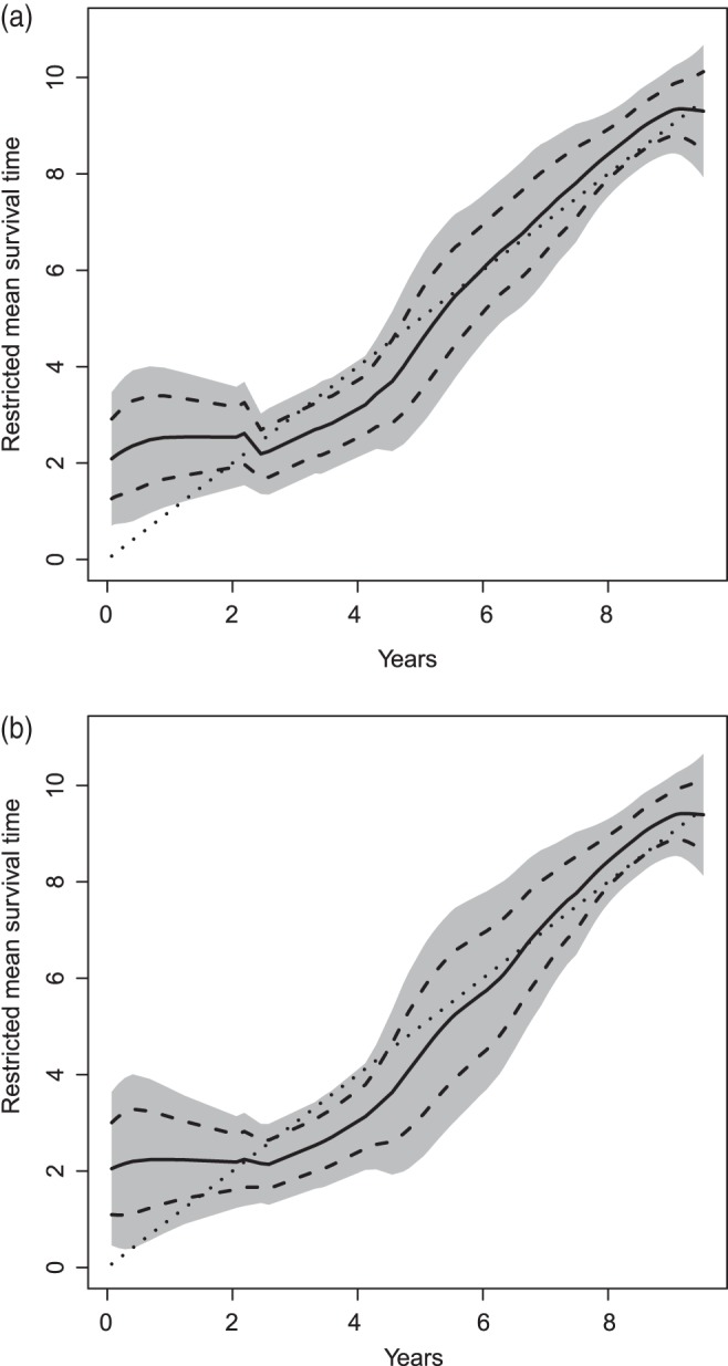
Estimated subject-specific restricted mean survival time (solid curve) over the score, and its 95% pointwise (dashed curve) and simultaneous confidence intervals (shaded region). The dotted line is the 45 reference line. The survival function of the censoring time C is estimated locally (a) and based on the entire sample (b).
As a conventional practice, we may stratify the subjects in the hold-out set into groups such as low, intermediate, and high risk groups by discretizing the continuous score. For example, we may create four classes based on the quartiles of the scores. Figure 4 presents the KM curves for these four strata. Visually these curves appear quite different. Moreover, their estimated RMETs and the standard error estimates (in parentheses) are 3.59 (0.46), 6.26 (0.53), 8.50 (0.40), and 9.14 (0.31) in years, respectively. These indicate that the scoring system does have reasonable discriminating capability with respect to the patients’ RMET. How to construct an “efficient” categorization of the existing scoring system warrants future research.
Fig. 4.
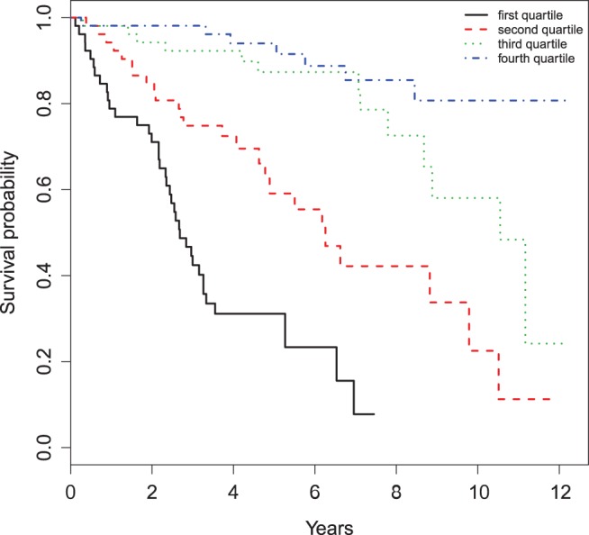
KM estimates of the survival functions of the four strata divided by quartiles of the scores based on the PBC data.
6. Remarks
In comparing two groups with censored event-time data, the point and interval estimates of the two RMETs and their counterparts for the group contrast provide much more clinically relevant information than, for example, the hazard ratio estimates. The results from the HIV data set from ACTG 320 discussed in Section 1 is a good example, in that the three-drug combination is statistically significantly better than the conventional therapy, but the gain from the new treatment with respect to RMET was not as impressive from a clinical standpoint, likely due to the relatively short follow-up time. Note that for this case, the median event time cannot be estimated empirically due to heavy censoring. Moreover, we cannot evaluate models using the individual predicted error, such as the  distance function, with the median event time. It follows that the RMET is probably among the most meaningful, model-free, global measures for the distribution of the event time to evaluate the treatment efficacy. The choice of τ to define the RMET is crucial, which may be determined at the study design stage with respect to clinical relevance and feasibility of conducting the study.
Note that one of the attractive features of the model which directly relates the RMET to its covariates proposed here is that the score created is free of the censoring distribution even when the model is not correctly specified. On the other hand, those scores built from the Cox or AFT models depend on the study-specific censoring distribution when the model is misspecified.
Supplementary material
Supplementary material is available at http://biostatistics.oxfordjournals.org.
Funding
The work is partially supported by the National Institutes of Health grants (R01 AI052817, RC4 CA155940, U01 AI068616, UM1 AI068634, R01 AI024643, U54 LM008748, R01 HL089778) and contracts.
Supplementary Material
Acknowledgements
We are grateful to the Editor, Associate Editor, two referees, and Dr Brian Claggett for constructive comments on the paper. Conflict of Interest: None declared.
References
- Andersen P. K., Hansen M. G., Klein J. P. Regression analysis of restricted mean survival time based on pseudo-observations. Lifetime Data Analysis. 2004;10(4):335–350. doi: 10.1007/s10985-004-4771-0. [DOI] [PubMed] [Google Scholar]
- Cai T., Tian L., Uno H., Solomon S. D., Wei L. J. Calibrating parametric subject-specific risk estimation. Biometrika. 2010;97(2):389–404. doi: 10.1093/biomet/asq012. [DOI] [PMC free article] [PubMed] [Google Scholar]
- Chen P. Y., Tsiatis A. A. Causal inference on the difference of the restricted mean lifetime between two groups. Biometrics. 2001;57(4):1030–1038. doi: 10.1111/j.0006-341x.2001.01030.x. [DOI] [PubMed] [Google Scholar]
- Cox D. R. Regression models and life-tables (with discussion) Journal of the Royal Statistical Society, Series B. 1972;34:187–220. [Google Scholar]
- Dabrowska D. M. Non-parametric regression with censored survival time data. Scandinavian Journal of Statistics. 1987;14(3):181–197. [Google Scholar]
- Dabrowska D. M. Uniform consistency of the kernel conditional Kaplan–Meier estimate. The Annals of Statistics. 1989;17(3):1157–1167. [Google Scholar]
- Fleming T. R., Harrington D. P. Counting Processes and Survival Analysis. Vol. 8. New York: Wiley Online Library; 1991. [Google Scholar]
- Gilbert P. B., Wei L. J., Kosorok M. R., Clemens J. D. Simultaneous inferences on the contrast of two hazard functions with censored observations. Biometrics. 2002;58:773–780. doi: 10.1111/j.0006-341x.2002.00773.x. [DOI] [PubMed] [Google Scholar]
- Hammer S. M., Squires K. E., Hughes M. D., Grimes J. M., Demeter L. M., Currier J. S., Eron J. J., Feinberg J. E., Balfour H. H., Deyton L. R. A controlled trial of two nucleoside analogues plus indinavir in persons with human immunodeficiency virus infection and cd4 cell counts of 200 per cubic millimeter or less. New England Journal of Medicine-Unbound Volume. 1997;337(11):725–733. doi: 10.1056/NEJM199709113371101. and others. [DOI] [PubMed] [Google Scholar]
- Jin Z., Lin D. Y., Wei L. J., Ying Z. Rank-based inference for the accelerated failure time model. Biometrika. 2003;90(2):341–353. [Google Scholar]
- Kalbfleisch J. D., Prentice R. L. The Statistical Analysis of Failure Time Data. New York: John Wiley & Sons; 2002. [Google Scholar]
- Lin D. Y., Wei L. J. The robust inference for the Cox proportional hazards model. Journal of American Statistical Association. 1989;84:1074–1078. [Google Scholar]
- Park B. U., Kim W. C., Ruppert D., Jones M. C., Signorini D. F., Kohn R. Simple transformation techniques for improved non-parametric regression. Scandinavian Journal of Statistics. 1997;24(2):145–163. [Google Scholar]
- Royston P., Parmar M. K. B. The use of restricted mean survival time to estimate the treatment effect in randomized clinical trials when the proportional hazards assumption is in doubt. Statistics in Medicine. 2011;30(19):2409–2421. doi: 10.1002/sim.4274. [DOI] [PubMed] [Google Scholar]
- Rudser K. D., LeBlanc M. L., Emerson S. S. Distribution-free inference on contrasts of arbitrary summary measures of survival. Statistics in Medicine. 2012;31(16):1722–1737. doi: 10.1002/sim.4505. [DOI] [PubMed] [Google Scholar]
- Therneau T. M., Grambsch P. M. Modeling Survival Data: Extending the Cox Model. Berlin: Springer; 2000. [Google Scholar]
- Tian L., Cai T., Goetghebeur E., Wei L. J. Model evaluation based on the sampling distribution of estimated absolute prediction error. Biometrika. 2007;94(2):297–311. [Google Scholar]
- Tian L., Zucker D., Wei L. J. On the Cox model with time-varying regression coefficients. Journal of the American Statistical Association. 2005;100(469):172–183. [Google Scholar]
- Tsiatis A. A. Estimating regression parameters using linear rank tests for censored data. The Annals of Statistics. 1990;18(1):354–372. [Google Scholar]
- Zhao H., Tsiatis A. A. A consistent estimator for the distribution of quality adjusted survival time. Biometrika. 1997;84(2):339–348. [Google Scholar]
- Zhao H., Tsiatis A. A. Efficient estimation of the distribution of quality-adjusted survival time. Biometrics. 1999;55(4):1101–1107. doi: 10.1111/j.0006-341x.1999.01101.x. [DOI] [PubMed] [Google Scholar]
- Zhao L., Tian L., Uno H., Solomon S. D., Pfeffer M. A., Schindler J. S., Wei L. J. Utilizing the integrated difference of two survival functions to quantify the treatment contrast for designing, monitoring, and analyzing a comparative clinical study. Clinical Trials. 2012;9(5):570–577. doi: 10.1177/1740774512455464. [DOI] [PMC free article] [PubMed] [Google Scholar]
Associated Data
This section collects any data citations, data availability statements, or supplementary materials included in this article.