

Abstract
FMRI data are acquired as complex-valued spatiotemporal images. Despite the fact that several studies have identified the presence of novel information in the phase images, they are usually discarded due to their noisy nature. Several approaches have been devised to incorporate magnitude and phase data, but none of them has performed between-group inference or classification. Multiple kernel learning (MKL) is a powerful field of machine learning that finds an automatic combination of kernel functions that can be applied to multiple data sources. By analyzing this combination of kernels, the most informative data sources can be found, hence providing a better understanding of the analyzed learning task. This paper presents a methodology based on a new MKL algorithm (ν-MKL) capable of achieving a tunable sparse selection of features’ sets (brain regions’ patterns) that improves the classification accuracy rate of healthy controls and schizophrenia patients by 5% when phase data is included. In addition, the proposed method achieves accuracy rates that are equivalent to those obtained by the state of the art lp-norm MKL algorithm on the schizophrenia dataset and we argue that it better identifies the brain regions that show discriminative activation between groups. This claim is supported by the more accurate detection achieved by ν-MKL of the degree of information present on regions of spatial maps extracted from a simulated fMRI dataset. In summary, we present an MKL-based methodology that improves schizophrenia characterization by using both magnitude and phase fMRI data and is also capable of detecting the brain regions that convey most of the discriminative information between patients and controls.
Keywords: complex-valued fMRI data, multiple kernel learning, feature selection, independent component analysis, support vector machines, schizophrenia
1. Introduction
Functional magnetic resonance imaging (fMRI) data are acquired at each scan as a bivariate complex image pair for single-channel coil acquisition, containing both the magnitude and the phase of the signal. This complex-valued spatiotemporal data have been shown to contain physiologic information (Hoogenraad et al., 2001). In fact, it has been shown that there are activation-dependent differences in the phase images as a function of blood flow, especially for voxels with larger venous blood fractions (Hoogenraad et al., 1998). Based on these findings and on results of some models that showed that phase changes arise only from large non-randomly oriented blood vessels, previous work has focused on filtering voxels with large phase changes (Nencka and Rowe, 2007; Menon, 2002; Zhao et al., 2007). Nonetheless, more recent studies provide evidence that the randomly oriented microvasculature can also produce non-zero blood-oxygen-level-dependent (BOLD)-related phase changes (Feng et al., 2009; Zhao et al., 2007), suggesting that the phase information contains useful physiologic information. Furthermore, previous studies have reported task-related fMRI phase changes (Hoogenraad et al., 2001; Menon, 2002). The previously discussed findings on the literature provide evidence that phase incorporates information that may help us better understand brain function. For this reason, the present study explores whether phase could improve the detection of functional changes in the brain when combined with magnitude data.
While both magnitude and phase effects are generated by the blood-oxygen-level-dependent mechanism and they both depend on the underlying vascular geometry and the susceptibility change, they primarily depend on different magnetic field characteristics (Calhoun and Adali, 2012). To first order, the magnitude attenuation depends on the intra-voxel magnetic field inhomogeneity and the phase depends on the mean magnetic field at the voxel. For this reason, it makes sense to think that the inclusion of the phase along with the magnitude could increment the sensitivity to detect informative regions and better discriminate control and patient subjects. Although phase could potentially provide complementary information to magnitude data, most studies discard the phase data. The phase images are usually discarded since their noisy nature poses a challenge for a successful study of fMRI when the processing is performed in the complex domain (Calhoun et al., 2002).
Nonetheless, some studies, such as Rowe (2005); Calhoun et al. (2002), have tried to incorporate phase data on fMRI analyses, but neither of these papers evaluated phase changes at group level. The work in Arja et al. (2010) presents a group analysis to evaluate task-related phase changes compared to the task-related magnitude changes in both block-design and event-related tasks. The detection of phase activation in the regions expected to be activated by the task provides further motivation to implement methods that focus on combining magnitude and phase data to achieve better group inferences.
Methods that are capable of combining different data sources can be applied to fMRI in order to efficiently use the information present in the magnitude and phase of the data. Such methods should also consider that fMRI data, though high dimensional, show sparsely distributed activation in the brain. In other words, a significant number of voxels will not convey information of brain activity. Moreover, informative voxels are likely to be distributed in clusters or brain regions. For these reasons, an adequate method to combine magnitude and phase fMRI data should also be able to automatically select the regions that characterize the condition under study.
Among the various approaches that are well-suited to solve this problem, group least angle shrinkage and selection operator (Group LASSO) (Yuan and Lin, 2006) or nonlinear approaches such as multiple kernel learning (MKL) methods (Gönen and Alpaydin, 2011) are the most commonly used methods to carry out group or kernel selection. In particular, MKL algorithms can be used to do group selection if a kernel is defined on each group. There are two advantages of applying kernels to different groups on fMRI data. On the one hand, one can exploit linear or nonlinear relationships among the voxels of the same group just by using linear (Euclidean dot product) or nonlinear kernels. On the other hand, MKL admits a dual formulation, in such a way that the computational complexity of the problem is defined by the number of samples rather than the number of voxels per sample. For fMRI data, this translates into a dramatic complexity reduction with respect to the primal formulation.
Several MKL algorithms have been devised in the last decade. The optimization of a weighted linear combination of kernels for the support vector machine (SVM) was proposed in Lanckriet et al. (2004). Their formulation reduces to a convex optimization problem, namely a quadratically-constrained quadratic program (QCQP). Later, Bach et al. (2004) proposed a dual formulation of this QCQP as a second-order cone programming problem, which improved the running time of the algorithm. Afterwards, Sonnenburg et al. (2006) reformulated the algorithm proposed by Bach et al. as a semi-infinite linear program, which amounts to repeatedly training an SVM on a mixture kernel while iteratively refining the kernel coefficients. The above mentioned algorithms attempt to achieve sparsity by promoting sparse solutions in terms of the kernel coefficients. Specifically, both Bach et al. (2004) and Sonnenburg et al. (2006) enforced sparsity by using l1-norm regularization terms on these coefficients, an approach that has exhibited certain limitations for linear SVM (Zhu and Zou, 2007; Wang et al., 2009). Alternative solutions can be found in Kloft et al. (2011), where a non-sparse MKL formulation based on an lp-norm regularization term on the kernel coefficients (with p ≥ 1) is introduced, or in Orabona and Jie (2011), which mixes elements of lp-norm and elastic net regularization.
Keeping in mind the aforementioned reasoning, the aim of the present work is to differentiate groups of healthy controls and schizophrenia patients from an auditory oddball discrimination (AOD) task by efficiently combining magnitude and phase information. To do so, we propose a novel MKL formulation that automatically selects the regions that are relevant for the classification task. First, we apply group independent component analysis (ICA) (Calhoun et al., 2001) separately to both magnitude and phase data to extract activation patterns from both sources. Next, given the local-oriented nature of the proposed MKL methodology, local (per-region) recursive feature elimination SVM (RFE-SVM) (Guyon et al., 2002) is applied to magnitude and phase data to extract only their relevant information. Then, following the recursive composite kernels scheme presented in Castro et al. (2011), each one of the defined brain regions is used to construct a kernel, after which our proposed MKL formulation is applied to select the most informative ones. The novelty of this formulation, which is based on the work presented in Gómez-Verdejo et al. (2011), relies on the addition of a parameter (ν) that allows the user to preset an upper bound of the number of kernels to be included in the final classifier. We call this algorithm ν-MKL.
Based on this procedure, we present three possible variants of the algorithm. In the first one, the assumption of magnitude and phase data belonging to a joint distribution is adopted. Therefore, they are concatenated, RFE-SVM is applied to each region, and the selected voxels of each of them are used to construct the kernels. In the second one, RFE-SVM is applied independently to magnitude and phase for each region, after which the selected voxels are concatenated to construct kernels. In the third approach, we assume that magnitude and phase come from independent distributions, so RFE-SVM is applied independently to both of them and kernels are constructed from magnitude and phase data without concatenation. The second and third approaches are significantly different for nonlinear kernels. Concatenating the data prior to kernel computation assumes nonlinear dependencies between magnitude and phase, whereas computing separate kernels assumes linear dependence. For the case of linear kernels, the difference relies on the fact that separate kernels allow the algorithm to assign different weights (and thus different importance) to the magnitude and phase data representations of the regions.
The proposed approach is tested using linear and Gaussian kernels. In addition, the performance of ν-MKL is further evaluated by comparing its results in terms of classification accuracy with those obtained by applying lp-norm MKL (Kloft et al., 2011) and SVM. Furthermore, the estimates of the sparsity of the problem of both MKL algorithms are also used for comparison purposes. However, both the actual degree of sparsity of the real dataset and the degree of differential activity present on each region are unknown. For this reason, a simulated dataset where this information can be estimated a priori is generated to verify the capacity of ν-MKL to detect both the sparsity of the problem and the amount of information present in the analyzed brain regions, which is then compared to the one attained by lp-norm MKL.
2. Materials and Methods
2.1. FMRI data
2.1.1. Simulated dataset
This dataset, which is generated using the simulation toolbox for fMRI data (SimTB)1 (Allen et al., 2011), mimics the BOLD response of two groups of subjects with different brain activation patterns.
SimTB generates data under the assumption of spatiotemporal separability, i.e., that data can be expressed as the product of time courses and spatial maps. Default spatial maps are modeled after components commonly seen in axial slices of real fMRI data and most are created by combinations of simple Gaussian distributions, while time courses are constructed under the assumption that component activations result from underlying neural events as well as noise. Neural events can follow block or event-related experimental designs, or can represent unexplained deviations from baseline; these are referred to as unique events. The time course of each component is created by adding together amplitude-scaled task blocks, task events and unique events by means of modulation coefficients, as shown in Fig. 1.
Figure 1.
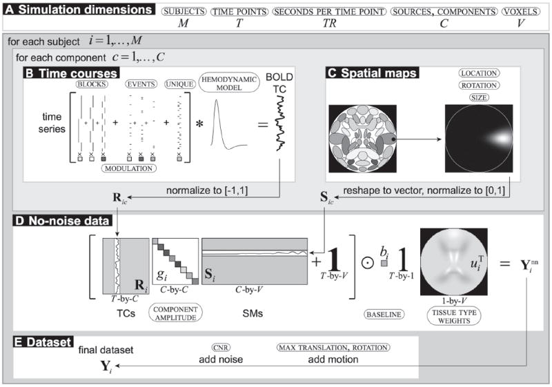
Block diagram of the data generation process followed by SimTB. (A) Simulation dimension is determined by the number of subjects, time points, components and voxels. (B) Time courses are the sum of amplitude-scaled task block, task event, and unique event time series modeled into a BOLD time course. (C) Spatial maps are selected, translated, rotated, resized, and normalized. (D) The noise-free data combines time courses and spatial maps by component amplitudes, and scaled to a tissue type weighted baseline. (E) The final dataset includes motion and noise. (Modified from Allen et al. (2011))
The generated experimental design is characterized by the absence of task events, the BOLD response being characterized by unique events only, thus being similar to a resting-state experiment. The spatial maps generated for all components did not exhibit any consistent changes among groups, the exception being the default mode network. For this specific component, changes in the activation coefficients between groups were induced by slightly shifting them in the vertical axis. By doing so, it is expected that differential activation is generated in the voxels within the Gaussian blobs representing the anterior and posterior cingulate cortex as well as the left and right angular gyri.
The experimental design is simulated for two groups of M = 200 subjects, each subject with C = 20 components in a data set with V = 100 × 100 voxels and T = 150 time points collected at TR = 2 seconds. Among the 30 components available by default on SimTB, we did not include in the simulation those associated with the visual cortex, the precentral and postcentral gyri, the subcortical nuclei and the hippocampus. To mimic between-subject spatial variability, the components for each subject are given a small amount of translation, rotation, and spread via normal deviates.
Translation in the horizontal and vertical directions of each source have a standard deviation of 0.1 voxels, except for the default mode network. This component has different vertical translation between groups. Both of them have a standard deviation of 0.5 voxels, but different means (0.7 and -0.7 for groups 1 and 2, respectively). In addition, rotation has a standard deviation of 1 degree, and spread has a mean of 1 and standard deviation of 0.03.
All components have unique events that occur with a probability of 0.5 at each TR and unique event modulation coefficients equal to 1. At the last stage of the data generation pipeline, Rician noise is added to the data of each subject to reach the appropriate CNR level, which is equal to 0.3 for all subjects.
2.1.2. Complex-valued real dataset
Participants
Data were collected at the Mind Research Network (Albuquerque, NM) from healthy controls and patients with schizophrenia. Schizophrenia was diagnosed according to DSM-IV-TR criteria (American Psychiatric Association, 2000) on the basis of both a structured clinical interview (SCID) (First et al., 1995) administered by a research nurse and the review of the medical file. All patients were on stable medication prior to the scan session. Healthy participants were screened to ensure they were free from DSM-IV Axis I or Axis II psychopathology using the SCID for non-patients (Spitzer et al., 1996) and were also interviewed to determine that there was no history of psychosis in any first-degree relatives. All participants had normal hearing, and were able to perform the AOD task successfully during practice prior to the scanning session.
The set of subjects is composed of 21 controls and 31 patients. Controls aged 19 to 40 years (mean=26.6, SD=7.4) and patients aged 18 to 49 years (mean=27.7, SD=8.2). A two-sample t-test on age yielded t = 0.52 (p-value = 0.60). There were 8 male controls and 21 male patients.
Experimental Design
The subjects followed a three-stimulus AOD task; two runs of 244 auditory stimuli consisting of standard, target, and novel stimuli were presented to the subject. The standard stimulus was a 1000-Hz tone, the target stimulus was a 1500-Hz tone, and the novel stimuli consisted of non-repeating random digital noises. The target and novel stimuli each was presented with a probability of 0.10, and the standard stimuli with a probability of 0.80. The stimulus duration was 200 ms with a 2000-ms stimulus onset asynchrony. Both the target and novel stimuli were always followed by at least 3 standard stimuli. Steps were taken to make sure that all participants could hear the stimuli and discriminate them from the background scanner noise. Subjects were instructed to respond to the target tone with their right index finger and not to respond to the standard tones or the novel stimuli.
Image Acquisition
FMRI imaging was performed on a 1.5 T Siemens Avanto TIM system with a 12-channel radio frequency coil. Conventional spin-echo T1-weighted sagittal localizers were acquired for use in prescribing the functional image volumes. Echo planar images were collected with a gradient-echo sequence, modified so that it stored real and imaginary data separately, with the following parameters: FOV = 24 cm, voxel size = 3.75 × 3.75 × 4.0 mm3, slice gap = 1 mm, number of slices = 27, matrix size = 64 × 64, TE = 39 ms, TR = 2 s, flip angle = 75°. The participant’s head was firmly secured using a custom head holder. The two stimulus runs consisted of 189 time points each, the first 6 images of each run being discarded to allow for T1 effects to stabilize.
2.2. Data processing
The analysis pipelines of both the simulated and the complex-valued fMRI datasets are shown in Fig. 2. The processing stages that are applied to these datasets are explained in what follows.
Figure 2.
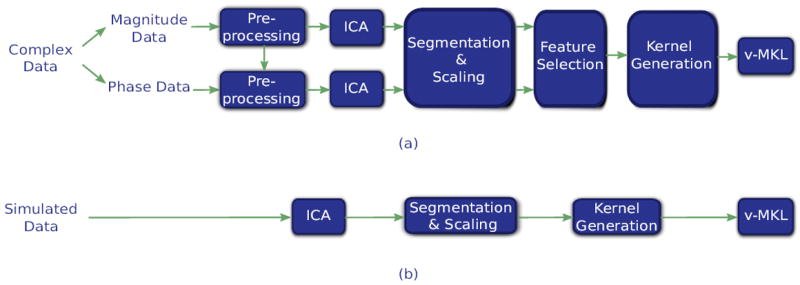
Data processing stages of (a) the complex-valued fMRI dataset and (b) the simulated dataset. On the preprocessing stage of the complex-valued fMRI data, motion correction and spatial normalization parameters were computed from the magnitude data and then applied to the phase data. Next, ICA was applied to magnitude and phase data separately, a single component being selected for each data source. Individual subject components were then back-reconstructed from the group ICA maps of each run (2 ICA maps per subject for each data source).
2.2.1. Preprocessing
The magnitude and phase images were written out as 4D NIfTI (Neuroimaging Informatics Technology Initiative) files using a custom reconstruction program on the scanner. Preprocessing of the data was done using the SPM5 software package2. The phase images were unwrapped by creating a time series of complex images (real and imaginary) and dividing each time point by the first time point, and then recalculating the phase images. Further phase unwrapping was not required. Magnitude data were co-registered using INRIAlign (Freire and Mangin, 2001; Freire et al., 2002) to compensate for movement in the fMRI time series images. Images were then spatially normalized into the standard Montreal Neurological Institute (MNI) space (Friston et al., 1995). Following spatial normalization, the data (originally acquired at 3.75 × 3.75 × 4 mm3) were slightly upsampled to 3 × 3 × 3 mm3, resulting in 53 × 63 × 46 voxels. Motion correction and spatial normalization parameters were computed from the magnitude data and then applied to the phase data. The magnitude and phase data were both spatially smoothed with a 10 × 10 × 10 − mm3 full-width at half-maximum Gaussian filter. Phase and magnitude data were masked to exclude non-brain voxels.
2.2.2. Group spatial ICA
As shown in Fig. 2, group spatial ICA (Calhoun et al., 2001) is applied to both the simulated and the complex-valued fMRI datasets to decompose the data into independent components using the GIFT software3. Group ICA is used due to its extensive application to fMRI data for schizophrenia characterization (Kim et al., 2008; Demirci et al., 2009; Calhoun et al., 2006). We also attempted to train the proposed method with activation maps retrieved by the general linear model, but it performed better when provided with ICA data.
ICA was applied to magnitude and phase data separately for the complex-valued fMRI dataset. Dimension estimation, which was used to determine the number of components, was performed using the minimum description length criteria, modified to account for spatial correlation (Li et al., 2007). For both data sources, the estimated number of components was 20. Data from all subjects were then concatenated and this aggregate data set reduced to 20 temporal dimensions using principal component analysis (PCA), followed by an independent component estimation using the infomax algorithm (Bell and Sejnowski, 1995). Individual subject components were then back-reconstructed from the group ICA analyses to retrieve the spatial maps (ICA maps) of each run (2 AOD task runs) for each data source.
To reduce the complexity of the analysis of magnitude and phase data, a single component was selected for each data source. These components were selected as follows. For magnitude data, we found three task-related components: the temporal lobe component (t-value=13.8, p-value=5.88 × 10⁻¹⁹), the default mode network (t-value=−11.0, p-value=4.57 × 10⁻¹⁵) and the motor lobe component (t-value=8.0, p-value=1.47 × 10⁻¹⁰). Among these three candidates, the most-discriminative task-related component was selected within a nested cross-validation (CV) procedure; this is explained on detail on section 2.3.5. For phase data, we only found one task-related component: the posterior temporal lobe component (t-value=-2.29, p-value=0.02). While phase data does not show as strong a task response as magnitude data, it appears to be useful for discriminative purposes.
On the other hand, the simulated dataset was decomposed into 20 components as follows. First, data from all subjects were temporally concatenated into a group matrix, being reduced to 20 temporal dimensions by using PCA. Then, an independent component estimation was applied to these reduced aggregate dataset using the infomax algorithm. Finally, individual subject components were back-reconstructed from the group ICA analysis.
To make the analysis of the simulated data resemble that of the complex-valued data as much as possible, the subjects’ ICA maps associated to a single component were analyzed for this dataset. This component was the default mode network, which was modeled to present differential activity between groups, as explained in section 2.1.1.
2.2.3. Data segmentation and scaling
As shown in Fig. 2, data segmentation is applied to both datasets. For the complex-valued one, this is applied to the individual ICA maps associated to the magnitude component and the posterior temporal lobe component for phase data. One of the objectives of the proposed approach is to locate the regions that better characterize schizophrenia through a multivariate analysis. To do so, an appropriate brain segmentation needs to be used. An adequate segmentation would properly capture functional regions in the brain and cover it entirely, as spatial smoothing may spread brain activation across neighboring regions. Unfortunately, anatomical templates such as the automated anatomical labeling (AAL) brain parcellation (Tzourio-Mazoyer et al., 2002) may not capture functional regions given their large spatial extent. In fact, these regions are defined by brain structure. Furthermore, they do not cover the entire brain.
One way of solving the problem of properly representing functional regions is to use a more granular segmentation of the brain. This could be attained by using a relatively simple cubical parcellation approach. We divided the brain into 9×9×9-voxel cubical regions; the first cube is located at the center of the 3-D array were brain data is stored and the rest of them are generated outwards, increasingly further from the center. A total number of 158 cubical regions containing brain voxels were generated by using a whole-brain mask together with the cubical parcellation. It should be highlighted that by applying this approach the data has not been downsampled, as the original voxels are preserved for posterior analysis. Another advantage of using the cubical regions instead of an anatomical atlas is that we do not incorporate prior knowledge of the segmentation of functional regions in the brain, letting the algorithm figure out automatically which regions are informative.
Our MKL-based methodology evaluates the information within regions under the assumption that active voxels are clustered, an inactive voxel being one with coefficients equal to zero across ICA maps for all subjects. This assumption would not hold for regions composed of few scattered voxels. To avoid such cases, those regions containing less than 10 active voxels were not considered valid and were not included in our analysis. Nonetheless, a post-hoc analysis of this threshold value showed that it does not significantly change the results of the proposed approach.
A similar segmentation procedure was used for the simulated dataset, where the analyzed spatial maps where divided into 9×9-voxel square regions. These data parcellation generated a total number of 109 square regions. Furthermore, each voxel activation level was normalized for both datasets. This was done by subtracting its mean value across subjects and dividing it by its standard deviation.
2.2.4. Region representation
For the complex-valued fMRI dataset, the ICA maps associated to magnitude and phase sources are segmented in cubical regions, while the ICA maps extracted from the simulated dataset are segmented in square regions, as stated in the previous section. The term region will be used hereafter to refer to either of these to be able to explain the following processing stages regardless of the analyzed dataset. Nonetheless, the procedure described on this section is applicable to the complex-valued dataset only.
Per-region feature selection is applied to magnitude and phase data either for single-source analysis or for data source combination. For the former case, local (per-region) RFE-SVM is directly applied to the analyzed data source, while for the combination of both sources local RFE-SVM (hereafter referred to simply as RFE-SVM) is applied to the data using two strategies:
The data from both magnitude and phase are concatenated prior to the application of RFE-SVM, under the assumption that both magnitude and phase data come from a joint distribution. We refer to this approach as joint feature selection.
RFE-SVM is applied independently to each data source. In this case, we assume that magnitude and phase come from independent distributions. We refer to this approach as independent feature selection.
2.2.5. Region characterization
The information within each region is characterized by means of a dot product matrix (Gram matrix in Euclidean space), which provides a pairwise measure of similarity between subjects for that region. This representation enables the selection of informative regions via an MKL formulation, which is explained in section 2.3.4.
As mentioned in the previous section, magnitude and phase are analyzed either separately or together. For single-source analysis, the generation of a Gram matrix for each region is straightforward. Conversely, three combination approaches are proposed to combine magnitude and phase data based on the used region representation. The first one computes the Gram matrix of each region right after joint feature selection is applied. The second one concatenates the outputs of independent feature selection for the computation of the Gram matrix, while the third one generates a Gram matrix from each output of the independent feature selection. This is graphically summarized on Fig. 3 and their rationale has already been discussed on the introduction.
Figure 3.
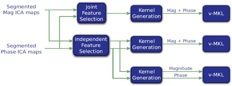
Strategies for complex-valued fMRI data feature selection and data sources combination. (Top row) First approach: Generation of a single kernel per brain region after the application of feature selection to the concatenation of the magnitude and phase brain region’s feature sets. (Middle row) Second approach: Feature selection is applied separately to the magnitude and phase brain region’s feature sets, after which they are concatenated and a single kernel per brain region is generated. (Bottom row) Third approach: Generation of one kernel per brain region for each data source after the independent application of feature selection to the magnitude and phase brain region’s feature sets.
We now provide a brief explanation of the application of dot products on regions’ data in the context of our proposed methodology. Let us assume that we are given N labeled training data (xi, yi), where the examples xi are represented as vectors of d features and yi ∈ {−1, 1}. In this case, the examples lie on χ = ℝd, which is called input space. Let us further assume that features are divided in L blocks such that ℝd = ℝd1 × … × ℝdL, so that each example xi can be decomposed into these L blocks, i.e., . In the case of our study, these blocks represent brain regions. Given two examples xi, xj, their data representations for region l are and , respectively. The dot product of these two examples for region l is defined by
which outputs a scalar value that equals 0 if both vectors are orthogonal.
Our proposed MKL approach is initially cast as a linear formulation to be optimized in dual space, although it is possible to solve its primal problem too. The reasons why we solve the dual problem are twofold. First, by working with the dual formulation the computational complexity of the problem is defined by the number of available data points instead of the number of features per data point. For fMRI data this amounts to a significant reduction in computational complexity with respect to the primal formulation. Second, the dual formulation can be easily extended to account for nonlinear relationships among voxels of a given region, as it is explained in section 2.3.4. However, increasing the model complexity is not guaranteed to be advantageous, due to the limited amount of data and their high dimensionality.
Normalization of kernels is very important for MKL as feature sets can be scaled differently for diverse data sources. In our framework, the evaluation of dot products on areas composed of different numbers of active voxels yields values in different scales. To compensate for that, unit variance normalization is applied to the computed Gram matrices.
More formally, let l be a region index and Kl be the Gram matrix associated to region l, i.e., . This matrix is normalized using the following transformation (Kloft et al., 2011):
| (1) |
2.3. Region selection based on a sparse MKL formulation
2.3.1. SVM formulation
Classical SVMs minimize a function that is composed of two terms. The first one is the squared norm of the the weight vector w, which is inversely proportional to the margin of the classification (Schölkopf and Smola, 2001). Hence, this term is related to the generalization capabilities of the classifier. The second term in the objective function is the empirical risk term, which accounts for the errors on the training data. Therefore, the SVM optimization problem can be expressed by
| (2) |
where slack variables ξi are introduced to allow some of the training observations to be misclassified or to lie inside the classifier margin and C is a constant that controls the tradeoff between the structural and empirical risk terms. This formulation can also be represented in dual space as
| (3) |
where . Here the kernel K is particularly defined as a Gram matrix because the proposed approach analyzes linear relationships within each region, as explained in section 2.2.5. Nonetheless, the presented MKL algorithm enables the usage of other kernels to analyze nonlinear relationships, as shown in section 2.3.4.
2.3.2. MKL problem
As shown in the previous section, SVMs represent the data using a single kernel. Alternatively, MKL represents the data as a linear combination of kernels, the parameters of this combination being learned by solving an optimization problem. In this paper, the idea is to optimize a linear combination of Gram matrices applied to different regions in dual space. The decision function of this problem is defined in the primal by
| (4) |
where x* is a given test pattern and wl are the parameters to be optimized.
2.3.3. Non-sparse MKL formulation
Several MKL approaches explicitly incorporate the coefficients of the linear combination of kernels in their primal formulations. In general, they include coefficients ηl such that K = Σl ηl Kl and add an l1-norm regularization constraint on η. The work presented in Kloft et al. (2011) proposes a non-sparse combination of kernels by using an lp-norm constraint with p > 1. For the specific case of the classification task introduced in section 2.2.5 this is their primal formulation:
| (5) |
and its dual formulation is given by
| (6) |
where and the notation is used as an alternative representation of s = [s1, …, sL]T for s ∈ ℝL.
2.3.4. An MKL formulation with block-sparsity constraints
The proposed MKL algorithm generates a block-sparse selection of features based on the idea of introducing primal variable sparsity constraints in the SVM formulation presented by Gómez-Verdejo et al. (2011).
Following that approach, block sparsity can be achieved by including additional constraints that upper bound the l2-norm of wl by a constant ε and slack variables γl. By adding these constraints we get this formulation:
| (7) |
A new cost term that is composed of the summation of slack variables γl weighted by a tradeoff parameter C′ is included in the formulation, a larger C′ corresponding to assigning a higher penalty to relevant blocks. Note that constraints ∥wl∥2 ≤ ε + γl, ∀l, allow group sparsity by loosely forcing the norm of each parameter block to be lower than ε. If ∥wl∥2 were assigned a value greater than ε in our scheme, γl would be strictly positive, increasing the value of the functional. Thus, on the one hand irrelevant regions that do not significantly decrease the empirical error term will simply be assigned a norm smaller than ε. On the other hand, terms ∥wl∥2 which are necessary to define the SVM solution will have values larger than ε. Blocks l such that ∥wl∥ ≤ ε are deemed irrelevant and they can be discarded, thereby providing block sparsity. As a consequence, null slack variables γl indicate the blocks to be removed.
To avoid CV of parameter ε, (7) has been reformulated to follow the ν-SVM introduced in Schölkopf et al. (2000),
| (8) |
This way, ε is optimized at the expense of introducing a new parameter ν ∈ (0, 1]. The advantage of including this new parameter relies on the fact that it is defined on a subset of ℝ, being much easier to be cross-validated than ε. Moreover, it can be demonstrated that ν fixes an upper bound for the fraction of slack variables γl allowed to be nonzero, so the user can even pre-adjust it if the number of regions to be selected is known a priori.
Let tl ∈ ℝ and ∥wl∥ ≤ tl ≤ ε + γl. By definition, (tl, wl) belongs to a second order cone in Vl = ℝdl+1. Therefore, as it is proven in Appendix B, for the optimization problem (8) the following second-order cone program dual problem holds:
| (9) |
where αi, 1 ≤ i ≤ N, and βl, 1 ≤ l ≤ L, are the dual variables applied to the empirical risk and block sparsity constraints in problem (8), respectively. While Appendix B analyzes the more general case in which Vl = ℝ × Hl, with Hl being a Hilbert space, the analysis presented on that appendix also holds for the linear case, where Vl = ℝdl+1. Furthermore, problem (9) is reduced to a canonical conic linear program formulation (see Appendix D) that can be solved using the MOSEK optimization toolbox4 (MOSEK ApS, 2007).
By analyzing the values of βl resulting from this optimization problem, the irrelevant regions can be found. Namely, ∥wl∥2 > ε if and only if (see Appendix C), so regions with βl values different from can be removed or their associated primal vector, wl, can be dropped to zero. The expression of the primal parameters of relevant regions is
| (10) |
where (see Appendix C for further details).
The estimated class of an unknown example x* can be computed by replacing (10) on (4)
| (11) |
where Iβ is the subset of the relevant regions (those ones with βl = C′/L) and the bias term b is computed as
| (12) |
where Iα = {i : 0 < αi < C}. While b can be estimated by using (12) for any i ∈ Iα, it is numerically safer to take the mean value of b across all such values of i (Burges, 1998).
Since the algorithm is described using a dual formulation that only uses dot products between data points, a nonlinear version of this algorithm can be directly constructed as follows. By applying a nonlinear transformation function φl(·) to the data points xi,l on region l, they can be mapped into a higher (possibly infinite) dimensional reproducing kernel Hilbert space (Aronszajn, 1950) provided with an inner product of the form . By virtue of the reproducing property, the dot product is a (scalar) expression depending only on the input data xi,l, xj,l, and it fits the Mercer’s theorem (see Appendix A). Such a function is called Mercer’s kernel. Thus, the formulation remains exactly the same, the only difference being the substitution of the scalar dot product by a Mercer’s kernel. One of the most popular Mercer’s kernels is the Gaussian kernel, with the expression .
Note that the use of Mercer’s kernels in the ν-MKL formulation exploits the nonlinear properties inside each region, while keeping linear combinations between them. ν-MKL is tested with both linear and Gaussian kernels for the complex-valued fMRI dataset, whereas linear kernels are used for the simulated dataset.
2.3.5. Parameter validation, feature selection and prediction accuracy estimation
Accuracy rate calculation, feature selection and parameter validation were performed by means of a nested K-fold CV, the latter two procedures being performed sequentially in the external CV. For the complex-valued dataset, K was set to 52 (leave-one-subject-out CV), while for the simulated dataset K = 10.
The external CV is used to estimate the accuracy rate of the classifier and the γ values associated to the informative regions as follows. At each round of the external CV, a subset of the data composed of a single fold is reserved as a test set (TestAll), the remaining data being used to train and validate the algorithm (labeled TrainValAll in Algorithm 1). Next, the most discriminative magnitude component of the three task-related ones is selected based on the error rate attained by each of them on an internal CV using a linear SVM, as shown in Algorithm 3. The component that achieves the minimum validation error is the one used to represent the magnitude source. It should be noted that lines 7 through 9 of Algorithm 1 are applied exclusively when magnitude-only or magnitude and phase data are analyzed. After doing so, feature selection is applied to the data using RFE-SVM. While this procedure is applied to the complex-valued dataset only as stated in section 2.2.4, we have incorporated it in Algorithm 1 as this is the only step that differs between both datasets in the nested K-fold CV.
It can be seen that RFE-SVM is applied at each round of the external CV to TrainValSel, i.e., the test set is never incorporated in this procedure, as it is a supervised algorithm. RFE-SVM then performs an internal CV to validate the selection of informative features. Within this validation procedure, a linear SVM is initially trained with all of the features of a given region. At each iteration of RFE-SVM, 20% of the lowest ranked features are removed, the last iteration being the one where the analyzed voxel set is reduced to 10% of its initial size.
After applying feature selection to the data, which yields the reduced sets TrainValRed and TestRed, TrainValRed is further divided into training and validation sets (see Algorithm 2), the latter one being composed of data from a single fold of TrainValRed. The classifier is then trained with a pool of parameter values for C, C′ and, ν, the validation error being estimated for each parameter combination as shown in Algorithm 2. The above process was repeated for all folds in TrainValRed, being the optimal tuple the one that achieved the minimum mean validation error. Then, the optimal tuple (C, C′, ν) was used to retrain ν-MKL (see Algorithm 1) and retrieve the γ values associated to each region for the current CV round.
Next, the test error rate is estimated in the reserved test set. After doing so, another fold is selected as the new test set and the entire procedure is repeated for each of them. The test accuracy rate is then estimated by averaging the accuracy rates achieved by each test set and the γ values associated to each region across CV rounds are retrieved. Please refer to Appendix C for details on the estimation of γ.
The criteria used to define the pool of values used for ν-MKL parameter selection was the following. The error penalty parameter C was selected from the set of values {0.01, 0.1, 1, 10, 100}, while the the sparsity tradeoff parameter C′ was selected from a set of 4 values in the range [0.1C, 10C], thus being at least one order of magnitude smaller than C but at most one order of magnitude higher. On the other hand, the set of values of the sparsity parameter ν were defined differently according to the analyzed dataset.
Since we had no prior knowledge of the degree of sparsity of the complex-valued dataset, ν was selected from the set of values {0.3, 0.5, 0.7, 0.9}. We also evaluated nonlinear relationships in each region by using Gaussian kernels, which additionally required the validation of σ. For each iteration of Algorithm 1, the median of the distances between examples of TrainValSet (σmed) was estimated. This value was then multiplied by different scaling factors to select the optimal value of σ on Algorithm 2, the scaling factor being validated from a set of three logarithmically spaced values between 1 and 10.
To get a better idea of the sparsity of the simulated data classification task, the mean of the spatial maps across subjects was generated and thresholded, as shown in Fig. 4(a). As stated in section 2.1.1, differential activation should be generated in the voxels within the Gaussian blobs of the default mode component, thus generating a sparse problem. However, the actual sparsity of this problem cannot be fully characterized mainly due to the high variance (compared to the mean) of the within-group vertical translation and the spread introduced on this component, which changes the location and the extent of these blobs. Nonetheless, by analyzing the regions that overlap with the map in Fig. 4(a), we can get a coarse estimate of its sparsity. It can be seen from Fig. 4(b) that the sparsity is higher than 10%. Based on this observation, we selected ν from the set of values {0.2, 0.4, 0.6, 0.8, 1}.
Figure 4.
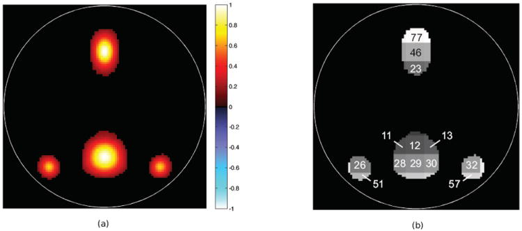
Mean spatial map of the default mode component and indexes of overlapping square regions. This figure shows (a) the default mode component’s thresholded mean spatial map across subjects and (b) the square regions that overlap with this mean map and the indexes of the overlapping regions.
Algorithm 1 Test ν-MKL
Inputs: DataSet, νυals, , Cυals
Outputs: TestAcc, γ
Define N: number of folds in DataSet
for i = 1 to N do
Extract TrainValAll (i) from DataSet
Extract TestAll (i) from DataSet
*Select Magnitude Component(TrainValAll (i)) ⇒ CompInd
*TrainValAll (i)(CompInd) ⇒ TrainValSel (i)
*TestAll(i)(CompInd) ⇒ TestSel (i)
*RFE-SVM(TrainValSel(i)) ⇒ SelectFeat
*TrainValSel(i)(SelectFeat) ⇒ TrainValRed(i)
*TestSel(i)(SelectFeat) ⇒ TestRed(i)
Validate parameters ν − MKL (TrainValRed(i), νυals, , Cυals) ⇒ C, C′, ν
Train with TrainValRed(i), C′, ν and C ⇒ Trained ν − MKL, γ(i)
Test with TestRed(i) and Trained ν − MKL
Store accuracy rate ⇒ acc(i)
end for
Average acc(i) over i ⇒ TestAcc
Algorithm 2 Validate parameters ν-MKL
Inputs: TrainValRed, νυals, , Cυals
Outputs: C, C′, ν
for i = 1 to N − 1 do
Extract Train(i) from TrainValRed
Extract Val(i) from TrainValRed
for j = 1 to # do
for k = 1 to #νυals do
νsel = νυals(k)
for l = 1 to #Cυals do
Csel = Cυals(l)
Train with Train(i), , νsel and Csel ⇒ Trained ν − MKL
Test with Val(i) and Trained ν − MKL
Store error ⇒ e(i, j, k, l)
end for
end for
end for
end for
Average e(i, j, k, l) over i ⇒ e(j, k, l)
Find (j, k, l) that minimizes e(j, k, l) ⇒ (J, K, L)
νυals (K) ⇒ ν
Cυals (L) ⇒ C
Algorithm 3 Select Magnitude Component
Inputs: TrainValAll
Outputs: CompInd
for i = 1 to N − 1 do
Extract Train(i) from TrainValAll
Extract Val(i) from TrainValAll
for j = 1 to 3 do
Train with Train(i)(j) ⇒ TrainedSVM
Test with Val (i)(j) and TrainedSVM
Store error ⇒ e(i, j)
end for
end for
Average e(i, j) over i ⇒ e(j)
Find j that minimizes e(j) ⇒ CompInd
2.3.6. Estimation of informative regions
The value of γ associated to a given region indicates its degree of differential activity between groups. However, γ does not take values on a fixed numeric scale. Specifically, γ values of informative regions across rounds of CV could be scaled differently, preventing us from directly comparing them. To correct for this, γ values at each CV round were normalized by the maximum value attained at that round. By doing so, the most relevant region for a given CV round would achieve a normalized score of 1 and the mean of the normalized γ values across CV rounds could be estimated.
The degree of differential activity of a region can also be assessed by estimating the number of times this region is deemed relevant across CV rounds (selection frequency). One way of taking into account both the selection frequency and the mean of the normalized γ to estimate the degree of information carried by a region is to generate a ranking coefficient that is the product of both estimates. These three estimates are used to evaluate the relevance of the analyzed regions for both the complex-valued and the simulated datasets.
For the specific case of the simulated dataset, the incorporation of a small vertical translation between groups allows us to identify the location of certain regions that are differentially activated. However, numeric a priori estimates of the degree of differential activation of all the regions were needed to test how well ν-MKL detected the most informative ones. These estimates were generated by calculating their classification accuracy by means of a 10-fold CV using a linear SVM.
As it has been previously mentioned, brain data was segmented in cubical regions for the complex-valued dataset in order to be capable of performing a multivariate analysis that included all of the regions in the brain. However, it is difficult to interpret our results based on the relevance of cubical regions. One way of solving this problem was to map cubical regions and their associated γ values to anatomical regions defined by the AAL brain parcellation using the Wake Forest University pick atlas (WFU-PickAtlas)5 (Lancaster et al., 1997, 2000; Maldjian et al., 2003, 2004).
The mapping criterion is explained as follows. A cubical region was assumed to have an effective contribution to an anatomical one if the number of overlapping voxels between them was greater than or equal to 10% of the number of voxels of that cubical region. If this condition was satisfied, then the cube was mapped to this anatomical region. After generating the correspondence between cubical and anatomical regions, a weighted average of the γ values of the cubes associated to an anatomical region was computed and assigned to this region for each CV round.
2.3.7. Proposed data processing with lp-norm MKL and SVM
As it has been previously discussed, one of the goals of this work is to compare the performance of ν-MKL with other classifiers and MKL algorithms, such as SVMs and lp-norm MKL. To do so, the same data processing applied in the proposed approach was used for these two cases, thus simply replacing ν-MKL by either an SVM or lp-norm MKL. The only difference in the processing pipeline for SVM was that the generated kernels were concatenated prior to being input to the classifier. As it will be seen in the results section, ν-MKL with Gaussian kernels does not provide better results than those obtained using linear kernels. These results were predictable based on the limited number of available subjects on our dataset. For this reason, we considered it appropriate to evaluate lp-norm MKL and SVM using linear kernels only.
The SVM was trained using the LIBSVM software package6 (Chang and Lin, 2011), and the error penalty parameter C was selected from a pool of 10 logarithmically spaced points between 1 and 100. Additionally, the lp-norm MKL implementation code was retrieved from the supplementary material of Kloft et al. (2011), which is available at http://doc.ml.tu-berlin.de/nonsparse_mkl/, and was run under the SHOGUN machine learning toolbox7 (Sonnenburg et al., 2010). For both the simulated and complex-valued dataset we considered norms p ∈ {1, 4/3, 2, 4, ∞} and C ∈ [1, 100] (5 values, logarithmically spaced).
For the simulated dataset, the mean of the kernel weights of lp-norm MKL across CV rounds for each region were also retrieved to evaluate how well this algorithm detected the amount of information provided by them, as well as to compare it against ν-MKL based on this criterion.
2.3.8. Data analysis with global approaches
We also wanted to evaluate the performance of our local-oriented MKL methodology on the complex-valued dataset by comparing it against global approaches, which analyze activation patterns on the brain as a whole. Linear kernels were applied to the data for these approaches.
One straightforward global approach is the direct application of an SVM to the data without the application of per-region feature selection. Its performance was used as a benchmark for other approaches and was applied to either magnitude data, phase data or the concatenation of both. We refer to the concatenation of of whole-brain data from both sources as whole data. Another used approach was the application of global (whole-brain) RFE-SVM to the data. This algorithm was implemented such that 10% of the lowest ranked voxels were removed at each iteration of RFE-SVM.
In addition, global RFE-SVM was used to combine magnitude and phase data using two strategies. The first one concatenated data from magnitude and phase sources prior to the application of global RFE-SVM. On the other hand, the second one applied global RFE-SVM to each source independently for feature selection purposes, after which an SVM was trained with the output of feature selection. The concatenation of the data from both sources after the application of this feature selection procedure is referred to as filtered data.
2.3.9. Statistical assessment of the contribution of phase data
If an improvement in the classification accuracy rate were obtained by combining both magnitude and phase data, further analysis would be required to confirm that this increment was indeed statistically significant. The statistic to be analyzed would be the accuracy rate obtained by using both data sources.
Since the underlying probability distribution of this statistic is unknown, a nonparametric statistical test such as a permutation test (Good, 1994) would enable us to test the validity of the null hypothesis. In this case, the null hypothesis would state that the accuracy rate obtained by using magnitude and phase data should be the same as the one attained by working with these two data sources regardless of the permutation (over the subjects) of the phase signal.
Let Dm and Df be the labeled magnitude and phase data samples, respectively, and let CR(Dm, Df) be the classification accuracy rate obtained with these two data sources using one of the combination approaches described on section 2.2.5 and the prediction accuracy estimation presented on section 2.3.5. The permutation test generates all possible permutation sets of the phase data sample , 1 ≤ k ≤ N!, doing no permutation of the magnitude data sample Dm. Next, it computes the accuracy rates CR(Dm, ). The p-value associated to CR(Dm, Df) under the null hypothesis is defined as
| (13) |
where I(·) is the indicator function.
Due to the high computational burden of computing all possible permutations in the elements of , in practice only tens or hundreds of them are used in a random fashion. The observed p-value is defined as
| (14) |
where M is the number of used permutations. In this case, the exact p-value cannot be known but a 95% confidence interval (CI) around p̂ can be estimated (Opdyke, 2003)
| (15) |
3. Results
3.1. Simulated dataset
The prior estimates of the degree of differential activation present on a subset of regions are shown on the first column of Table 1, these regions being sorted from most to least discriminative. It can be seen that 11 out of the 15 reported regions are consistent with the assumption that most of the differential activity would be focused on those squares overlapping with the default mode network activation blobs, as shown in Fig. 4.
Table 1.
Estimation of the information of a subset of regions using linear kernels along with ν-MKL and lp-norm MKL for the simulated dataset. The metrics used to determine the amount of information of the regions by means of ν-MKL (mean of the normalized γ values) and lp-norm MKL (kernel weights’ mean) as well as their selection frequencies for each algorithm are reported. Both the normalized γ values and the kernel weights have been scaled so that their maximum values equal 1 to make the comparison easier. These coefficients are contrasted against the accuracy rates achieved by these regions using a linear SVM.
| Region | Linear SVM | ν-MKL | lp-norm MKL | ||
|---|---|---|---|---|---|
|
| |||||
| Acc. Rate | Sel. Freq. | Normalized γ | Sel. Freq. | Kernel Weights | |
| Square 26 | 0.81 | 1 | 1.00 | 1 | 0.91 |
| Square 46 | 0.78 | 1 | 0.95 | 1 | 0.91 |
| Square 32 | 0.77 | 1 | 0.99 | 1 | 1.00 |
| Square 77 | 0.76 | 1 | 0.91 | 1 | 0.72 |
| Square 29 | 0.76 | 1 | 0.76 | 1 | 0.67 |
| Square 23 | 0.76 | 1 | 0.71 | 1 | 0.81 |
| Square 12 | 0.75 | 1 | 0.75 | 1 | 0.53 |
| Square 57 | 0.69 | 1 | 0.54 | 0.50 | 0.58 |
| Square 51 | 0.68 | 1 | 0.52 | 1 | 0.34 |
| Square 30 | 0.67 | 1 | 0.24 | 0.50 | 0.34 |
| Square 107 | 0.63 | 0.60 | 0.08 | 0.60 | 0.30 |
| Square 13 | 0.60 | 0.60 | 0.09 | 0.50 | 0.38 |
| Square 44 | 0.57 | 0.30 | 0.13 | 0.90 | 0.29 |
| Square 37 | 0.56 | 0.10 | 0.09 | 0.90 | 0.24 |
| Square 20 | 0.54 | 0.10 | 0.07 | 0.80 | 0.22 |
This table also shows the selection frequency and the relevance estimates of these regions using ν-MKL (normalized γ) and lp-norm MKL (kernel weights). A classification accuracy rate of 0.90 and 0.85 is attained by ν-MKL and lp-norm MKL, respectively. In addition, the fraction of selected regions was 0.14 for ν-MKL and 0.50 for lp-norm MKL.
3.2. Complex-valued dataset
We present the results of both local-oriented and global approaches on Table 2. Accuracy rates of the proposed methodology using ν-MKL, lp-norm MKL and SVM for single-source analysis and different source combination approaches are listed along with the results obtained by the global approaches introduced in section 2.3.8.
Table 2.
Performance of the proposed methodology and global approaches on the complex-valued fMRI dataset. This table presents the classification accuracy (first row) and the sensitivity/specificity rates (second row) of our local-oriented methodology using ν-MKL lp-norm MKL and SVM for single-source data (magnitude or phase) and different source combination approaches. It also shows the results obtained by global approaches. Notice that SVM is applied to both the proposed approach and global approaches. The reported values are attained by these algorithms using linear kernels, except where noted.
| Classifier | Single Sources | Combined Sources | |||||||
|---|---|---|---|---|---|---|---|---|---|
|
| |||||||||
| Prop. Approach | Global Approach | Proposed Approach | Global Approaches | ||||||
|
| |||||||||
| Magn. | Phase | Magn. | Phase | Comb. 1 | Comb. 2 | Comb. 3 | Whole Data | Filt. Data | |
| SVM | 0.77 | 0.64 | 0.62 | 0.58 | 0.80 | 0.79 | 0.79 | 0.63 | 0.80 |
| 0.84/0.67 | 0.65/0.64 | 0.71/0.48 | 0.55/0.62 | 0.85/0.71 | 0.82/0.74 | 0.82/0.74 | 0.71/0.50 | 0.82/0.76 | |
|
| |||||||||
| Global | – | – | 0.76 | 0.61 | – | – | – | 0.80 | – |
| RFE-SVM | – | – | 0.81/0.69 | 0.63/0.57 | – | – | – | 0.92/0.62 | – |
|
| |||||||||
| ν-MKL | 0.80 | 0.70 | – | – | 0.76 | 0.76 | 0.85 | – | – |
| (linear) | 0.85/0.71 | 0.69/0.71 | – | – | 0.82/0.67 | 0.84/0.64 | 0.90/0.76 | – | – |
|
| |||||||||
| ν-MKL | 0.78 | 0.68 | – | – | 0.68 | 0.77 | 0.85 | – | – |
| (Gaussian) | 0.84/0.69 | 0.71/0.64 | – | – | 0.77/0.55 | 0.87/0.62 | 0.92/0.74 | – | – |
|
| |||||||||
| lp-norm | 0.78 | 0.64 | – | – | 0.76 | 0.72 | 0.84 | – | – |
| MKL | 0.84/0.69 | 0.66/0.62 | – | – | 0.82/0.67 | 0.73/0.71 | 0.90/0.74 | – | – |
It can be seen that by applying linear ν-MKL to magnitude and phase data using the third combination approach, an increment of 5% with respect to the magnitude-only data analysis is obtained. In this case, CR(Dm, Df) = 0.85. After generating 100 permutations we get p̂ = 0.01 and a 95% CI [0, 0.03] according to (14) and (15), respectively. Since p < α = 0.05, we can reject the null hypothesis at a significance level of 0.05. Consequently, the improvement in classification accuracy rate obtained by including phase data is statistically significant with 95% confidence level.
Table 3 shows the cubical regions’ selection sparsity achieved by ν-MKL and lp-norm MKL. It can be seen that a higher selection sparsity is attained by classifying the data with ν-MKL for single-source analysis and the third source combination approach.
Table 3.
Selection sparsity achieved by ν-MKL and lp-norm MKL on the complex-valued dataset. This table shows the fraction of valid selected regions (according to the criterion discussed in section 2.2.3) for both ν-MKL and lp-norm MKL for single-source analysis (magnitude or phase) and the third combination approach of both sources. The presented values are achieved by both algorithms using linear kernels, except where noted.
| Source | Fraction of valid selected regions
|
# of valid regions | ||
|---|---|---|---|---|
|
ν-MKL
|
lp-norm MKL | |||
| Linear | Gaussian | |||
| Magnitude | 0.69 | 0.71 | 0.90 | 135 (of 158) |
| Phase | 0.70 | 0.69 | 0.85 | 108 (of 158) |
| Mag + Phase | 0.74 | 0.75 | 0.95 | 243 (of 316) |
The most informative regions and their associated relevance estimates detected by ν-MKL using linear kernels are reported as follows. The ranking coefficients of a subset of the top 40% ranked regions for magnitude-only and magnitude and phase data analyses (combination approach 3) are color-coded and displayed on top of a structural brain map in Fig. 5. This figure provides a graphical representation of the spatial distribution of these regions. In addition, Table 4 provides the differential activity estimates of some of these regions, such as selection frequency and normalized γ. This table also reports ranking indexes, which enables the analysis of changes on the relative contribution of these regions across single-source and combined-source analyses.
Figure 5.
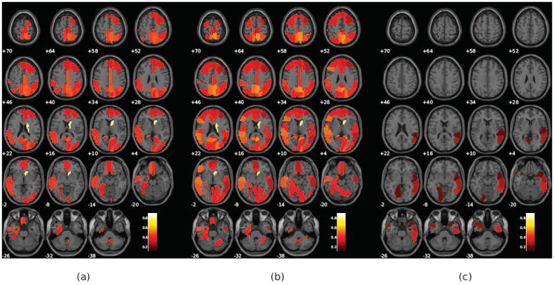
Ranking coefficients of a subset of the of the top 40% ranked regions for magnitude-only and magnitude and phase analyses. This figure shows (a) informative regions for the magnitude-only analysis, (b) informative regions of the magnitude source for the magnitude and phase analysis, and (c) informative regions of the phase source for the magnitude and phase analysis. Each of the displayed blobs are color-coded according to their associated ranking coefficients. As expected, magnitude is the most informative source, but several regions in phase, including the temporal lobe, are also informative.
Table 4.
Reduced set of the top 40% ranked regions for magnitude-only and magnitude and phase analyses and their differential activity estimates. This table lists a set of informative regions and their associated relevance estimates, such as selection frequency and normalized γ values. In addition, ranking indexes are reported to analyze changes on the relative contribution of these areas across single-source and combined-source analyses.
| Region | Single Source | Combined Sources | |||||||
|---|---|---|---|---|---|---|---|---|---|
|
| |||||||||
| Magnitude | Magnitude | Phase | |||||||
|
| |||||||||
| Rank | Sel. Freq. | Norm. γ | Rank | Sel. Freq. | Norm. γ | Rank | Sel. Freq. | Norm. γ | |
| Right Caudate Nucleus | 1 | 1.00 | 0.82 | 1 | 1.00 | 0.80 | – | – | – |
| Right Precuneus | 2 | 1.00 | 0.51 | 2 | 1.00 | 0.57 | – | – | – |
| Right Superior Occipital Gyrus | 3 | 1.00 | 0.49 | 3 | 1.00 | 0.53 | – | – | – |
| Right Middle Cingulate Gyrus | 4 | 0.98 | 0.49 | 15 | 1.00 | 0.43 | – | – | – |
| Right Superior Parietal Lobe | 5 | 1.00 | 0.48 | 8 | 1.00 | 0.48 | – | – | – |
| Left Gyrus Rectus | 6 | 0.96 | 0.49 | 12 | 0.98 | 0.44 | – | – | – |
| Right Angular Gyrus | 7 | 1.00 | 0.46 | 11 | 1.00 | 0.43 | – | – | – |
| Left Precuneus | 8 | 1.00 | 0.46 | 6 | 1.00 | 0.52 | – | – | – |
| Left Middle Temporal Gyrus | 9 | 1.00 | 0.45 | 7 | 1.00 | 0.50 | – | – | – |
| Left Superior Temporal Gyrus | 10 | 1.00 | 0.45 | 4 | 1.00 | 0.53 | – | – | – |
| Left Angular Gyrus | 11 | 1.00 | 0.44 | 20 | 1.00 | 0.40 | – | – | – |
| Left Parahippocampal Gyrus | 12 | 1.00 | 0.44 | 10 | 1.00 | 0.44 | – | – | – |
| Left Paracentral Lobule | 13 | 1.00 | 0.43 | 18 | 0.98 | 0.42 | – | – | – |
| Right Gyrus Rectus | 14 | 0.96 | 0.44 | 39 | 0.98 | 0.37 | – | – | – |
| Right Cuneus | 15 | 1.00 | 0.41 | 13 | 1.00 | 0.43 | – | – | – |
| Right Anterior Cingulate Gyrus | 23 | 0.96 | 0.39 | 35 | 0.98 | 0.38 | – | – | – |
| Left Hippocampus | – | – | – | 16 | 0.98 | 0.43 | – | – | – |
| Right Superior Temporal Gyrus | – | – | – | 23 | 1.00 | 0.39 | 88 | 0.96 | 0.23 |
| Left Superior Frontal Gyrus | – | – | – | 34 | 0.98 | 0.38 | – | – | – |
| Left Anterior Cingulate Gyrus | – | – | – | 36 | 0.98 | 0.38 | – | – | – |
| Left Middle Frontal Gyrus | – | – | – | 42 | 0.98 | 0.37 | – | – | – |
| Right Posterior Cingulate Gyrus | – | – | – | 50 | 0.98 | 0.34 | – | – | – |
| Left Posterior Cingulate Gyrus | – | – | – | 51 | 0.98 | 0.34 | – | – | – |
| Right Middle Temporal Gyrus | – | – | – | 62 | 0.98 | 0.31 | 72 | 0.98 | 0.29 |
| Right Inferior Temporal Gyrus | – | – | – | – | – | – | 56 | 0.98 | 0.33 |
| Left Temporal Pole: Middle Temporal Gyrus | – | – | – | – | – | – | 83 | 0.92 | 0.27 |
| Left Lingual Gyrus | – | – | – | – | – | – | 91 | 0.88 | 0.25 |
| Right Temporal Pole: Superior Temporal Gyrus | – | – | – | – | – | – | 92 | 0.94 | 0.23 |
4. Discussion
This work presents an MKL-based methodology that combines magnitude and phase data to better differentiate groups of healthy controls and schizophrenia patients from an AOD task. In contrast, previous approaches devised methods that incorporated magnitude and phase data, but did not perform between-group inferences. In addition, the presented methodology is capable of detecting the most informative regions for schizophrenia detection.
Table 2 shows the results obtained by our MKL-based methodology using ν-MKL for single-source analysis, as well as the combination of magnitude and phase. It can be seen that, when linear kernels are used, the first and the second combination approaches obtain a smaller classification accuracy rate compared to the magnitude-only analysis. On the contrary, the third approach achieves an increment of 5% with respect to the magnitude data analysis. The probability of this value being obtained by chance is in the range [0, 0.03], being statistically significant at the 95% confidence level. These results support the validity of the rationale behind the third combination approach, which assumed that magnitude and phase are dissimilar data, thus requiring a kernel mapping to be applied independently for each source.
The performance of ν-MKL was also evaluated using Gaussian kernels. These results are comparable to those obtained using linear kernels, except for combination 1. A detailed analysis of the parameter validation procedure revealed that the values of σ were usually 10 times σmed. Such a large value of σ makes the Gaussian kernel similar to a linear one, which is consistent with the reported results. In addition, these results suggest that adding complexity to the classification model is not helpful on this dataset. This finding comes as no surprise since our dataset is composed of data from a small number of subjects. However, it is expected that nonlinear kernels would better characterize schizophrenia if a bigger dataset were analyzed, In fact, the work presented in Castro et al. (2011) supports this postulate.
In addition to the results obtained by ν-MKL, Table 2 displays the results obtained by our local-oriented methodology using lp-norm MKL and SVM. The results obtained by ν-MKL seem to be equivalent or slightly better than those obtained by lp-norm MKL. The differences in classification accuracy for both algorithms do not seem to be statistically significant. However, we must keep in mind that this is not the only criterion used to compare the performance of both algorithms. These algorithms are also evaluated based on their capacity to detect the degree of differential activity of the analyzed regions and their capability to detect the sparsity of the classification task. In short, we analyze the capacity of both algorithms to achieve a better interpretation of the data. This is analyzed on more detail later on this section.
It can also be seen from Table 2 that both ν-MKL and lp-norm MKL appear to show a similar trend. For example, both algorithms obtain a classification accuracy rate below the one achieved by the magnitude-only analysis for the first and the second combination approaches; instead, SVM achieves a better classification result than magnitude data analysis for all combination approaches. This can be explained by the fact that SVM does not analyze the regions’ information locally since the data is concatenated prior to being input to the SVM.
The results obtained by using global approaches are shown on the same table. It can be seen that the two global RFE-SVM-based strategies used to combine magnitude and phase data also improve the classification accuracy rate obtained by processing magnitude data only. Furthermore, both of them reach the same rates (0.80). However, their rates are smaller than the one achieved by combination 3 of our local-oriented approach (0.85).
Another important objective of this work is to show that ν-MKL can better identify the feature sets that show discriminative activation between groups compared to other MKL algorithms, such as lp-norm MKL; the simulated dataset is used for this purpose. It was previously mentioned that the results in Table 1 indicate that 11 of the 15 reported regions do overlap with the default mode network activation blobs (Fig. 4). It should be noted that 10 out of those 11 regions, which show a significant differential activation according to the accuracy rates reported by SVM, are selected on all CV rounds by ν-MKL. In contrast, 2 of these regions (57 and 30) are selected by lp-norm MKL on only half of the CV rounds. On the other hand, the last three regions (44, 37 and 20), which show weak differential activation across groups, are selected by ν-MKL on a few CV rounds, whereas they achieve a high selection frequency with lp-norm MKL. Furthermore, it can be seen that the γ coefficients assigned by ν-MKL to these regions are approximately one order of magnitude smaller than the top ranked region (26), which is not the case for lp-norm MKL.
On section 2.3.7, we mention the validation of parameter p for lp-norm MKL experiments, this parameter being the norm of the kernel coefficients on one of the constraints imposed on (5). When p ≈ 1, these coefficients yield a kernel combination that is close to a sparse one, being actually sparse when p = 1. On the contrary, these coefficients are uniformly assigned the value 1 when p = ∞. We analyzed the validated values of p for each CV round in order to get a better idea of the reason why lp-norm MKL failed to give a better estimate of the contribution of the relevant areas on the simulated dataset. We found out that on 7 out of 10 rounds, p = 1 or 4/3 (close to 1). It is clear that lp-norm attempts to do a sparse selection of the informative regions, but with p ≈ 1 this algorithm seems to pick just some kernels when they are highly correlated, a limitation that would be consistent with the findings on l1-norm SVM (Wang et al., 2009). Even though lp-norm MKL looks for a sparse solution, it still estimates that the fraction of relevant regions is 0.50, deeming half of the regions of the analyzed spatial map informative. Based on the accuracy rate estimates obtained by a linear SVM and the graphical representation provided in Fig. 4, it is unlikely that the sparsity of the simulated data classification task is of that order. On the contrary, ν-MKL estimates that the fraction of relevant regions is 0.14, which seems more consistent with the prior knowledge of the spatial extent of the voxels having differential activation across groups.
Based on the analysis of the performance of both MKL algorithms on the simulated dataset, it can be inferred that the lp-norm MKL formulation based on a non-sparse combination of kernels provides a less precise estimate of the sparsity of the classification task at hand than ν-MKL. In addition, ν-MKL provides a more accurate measurement of the degree of information conveyed by each kernel.
If we analyze the results obtained for the complex-valued fMRI dataset, it can be seen that ν-MKL region selection is sparser than the lp-norm MKL one (Table 3), while still achieving at least equivalent classification results. A similar trend is found on the simulated dataset, with ν-MKL better detecting the sparsity of the classification task. Based on this finding, it can be argued that ν-MKL may achieve a better detection of the most informative brain regions on the complex-valued dataset. However, this cannot be verified as the ground truth for real fMRI data is unknown.
In terms of the selection of the most discriminative magnitude component, it should be highlighted that the default mode component was consistently selected at each iteration of Algorithm 1. This is an important finding that reinforces the notion that this spatial component reliably characterizes schizophrenia (Calhoun et al., 2008; Garrity et al., 2007).
Table 4 shows a reduced set of the most informative regions for magnitude-only and magnitude and phase analyses. Among the regions deemed informative by the former analysis temporal lobe regions can be found, which is consistent with findings on schizophrenia. To better understand which regions could be informative on our study, we need to be aware that the AOD task requires the subjects to make a quick button-press response upon the presentation of target stimuli. Such an action is highly sensitive to attentional selection and evaluation of performance, as the subject needs to avoid making mistakes. For this reason we highlight the presence of the anterior cingulate gyrus among the informative regions for the magnitude-only analysis, for it has been proposed that error-related activity in the anterior cingulate cortex is impaired in patients with schizophrenia (Carter et al., 2001). The presence of the precuneus and the middle frontal gyrus is also important, as it has been suggested that both regions are involved in disturbances in selective attention, which represents a core characteristic of schizophrenia (Ungar et al., 2010).
The regions that are deemed informative for magnitude only remain being the most informative when phase data is included in the analysis. However, their relative importance changes on several of them, as it can be seen by inspecting the rank values of these regions in these two scenarios. In addition, new brain areas show up in the set of informative regions, which is the case for some other temporal lobe regions and, for phase data, for regions of the temporal pole.
The presence of phase activation in regions expected to be differentially activated across groups in the AOD task, such as the temporal lobe regions, suggests that phase indeed provides reliable information to better characterize schizophrenia. In addition, it implies that the inclusion of phase can potentially increase sensitivity within regions also showing magnitude activation.
Similarly, the fact that regions of the temporal pole show up in the set of most informative regions is appealing, as evidence has been found that the temporal pole links auditory stimuli with emotional reactions (Clark et al., 2010). In fact, some studies report the temporal pole as a relevant component of the paralimbic circuit, and associate it with socioemotional processing (Crespo-Facorro et al., 2004). Since social cognition is a key determinant of functional disability of schizophrenia, it makes sense to hypothesize that the temporal pole is activated differently in schizophrenia patients when auditory stimuli is presented.
The aforementioned results reinforce the notion that magnitude and phase may be complementary data sources that can better characterize schizophrenia when combined.
5. Conclusions and Future Work
The presented methodology proposes a method to incorporate phase for fMRI data analysis. Nevertheless, there are other methods for complex-valued fMRI analysis that could be incorporated in our data analysis pipeline. Among those, we found the work presented in Rodriguez et al. (2012) especially appealing, as it could be used to extract complex-valued features to be used on our classification setting.
Another development that could be incorporated in our methodology is to extend it to do between-group inferences on non-categorical variables of interest by expanding ν-MKL to work with other loss functions. In addition, the algorithm could be reformulated so that it achieves better scalability with respect to sample size and number of kernels, as opposed to just implementing it to prove its functionality.
To the best of our knowledge, this is the first study to do classification using complex-valued fMRI data. This paper is an extension of the work presented in Arja et al. (2010), as it not only provides evidence that reinforces the idea that phase provides relevant information for group inferences, but it also extends it by showing that classification is improved for schizophrenia characterization if phase is analyzed together with magnitude. Furthermore, the proposed approach gives some insight of the classification results by providing scores associated to brain regions according to their relevance in the multivariate region analysis.
Highlights.
We propose a multiple kernel learning algorithm to process complex-valued fMRI data
Our method improves schizophrenia detection by including the phase of the fMRI data
This algorithm estimates the degree of differential activation of brain regions
The proposed algorithm outperforms the state of the art lp-norm MKL algorithm
Acknowledgments
We would like to thank the Mind Research Network for providing the data that was used by the approach proposed in this paper. This work has been supported by the following grants: NSF 0715022, NIH 1R01EB006841, and NIH 5P20RR021938.
Appendix A. Definition of Mercer’s Kernel
A theorem provided by Mercer (Aizerman et al., 1964) in the early 1900’s is of extreme relevance because it extends the principle of linear learning machines to the nonlinear case. The basic idea is that vectors x in a finite dimension space χ (called input space) can be mapped to a higher (possibly infinite) dimension Hilbert space H through a nonlinear transformation φ(·). By definition, a Hilbert space is a complete inner product space. A linear machine can be constructed in this higher dimensional space (Vapnik, 1998; Burges, 1998) (often called the feature space) which will be nonlinear from the point of view of the input space.
Mercer’s theorem shows that there exists a function φ : χ → H and an inner product
| (A.1) |
if and only if k(·, ·) satisfies Mercer’s condition.
A real-valued function k : χ × χ → ℝ is said to fulfill Mercer’s condition if for all square integrable functions g(x), i.e.,
| (A.2) |
the inequality
| (A.3) |
holds. Hilbert spaces provided with kernel inner products are often called reproducing kernel Hilbert spaces. In addition, the Gram matrix K generated by the available input vectors using kernel k(·, ·) (the kernel matrix) is positive semidefinite.
Appendix B. Lagrangian dual derivation
Recall that wl ∈ Hl and ∥wl∥2 ≤ tl ≤ ε + γl, where tl ∈ ℝ. Then, (tl, wl) ∈ Kl, where Kl ⊂ Vl = ℝ × Hl is a second-order cone (SOC) in Vl (Faybusovich and Mouktonglang, 2002). Thus, Eq. 8 can be restated as follows:
| (B.1) |
Since Kl is self-dual, the primal Lagrangian corresponding to the problem is
| (B.2) |
where α, μ, θ, σ, β, τ and δ are Lagrange multipliers (dual variables). Next, the partial derivatives with respect to the primal variables are computed and set to zero.
| (B.3) |
By replacing in Eq. B.2 the expressions obtained in Eq. B.3 the following dual Lagrangian function is obtained:
| (B.4) |
where maximizing LD with respect to the dual variables is equivalent to minimizing LP with respect to the primal variables.
Appendix C. Relevant blocks’ parameters values
The Karush-Kuhn-Tucker (KKT) optimality conditions of problem (B.1) were partially analyzed in Appendix B. Here we explore its complementary slackness equations.
The complementarity conditions for slack variables γl are defined by the equation τlγl = 0. The last partial derivative listed in Eq. B.3 yields . By combining these terms we get the following equation:
| (C.1) |
For the SOC Kl the following complementarity condition holds for the primal and dual variables:
| (C.2) |
i.e., the inner product of the primal and dual variables equals 0. By replacing the expressions for θl and σl found in Eq. B.3 and replacing them in the previous equation we get:
| (C.3) |
Another complementary slackness equation of interest is the one associated to the block sparsity constraints, which is defined by the following expression:
| (C.4) |
By simple inspection of these complementary slackness equations we can learn which values of βl indicate that a block l is informative (relevant) for the classification task. But first we need to know under which conditions Eq. C.2 holds. This equation is satisfied if and only if either of these two conditions are met:
One or both factors of the product are zero.
- Both factors are nonzero, belong to the boundary of Kl, and are anti-proportional (Bach et al., 2004); i.e., ∃ηl > 0 such that:
(C.5)
Recall from Appendix B that ∥wl∥2 ≤ tl ≤ ε + γl. Only those blocks l for which ∥wl∥2 > ε (γl > 0) are deemed relevant. We evaluated ∥wl∥2 for different values of βl by examining the complementary slackness equations and found the following 3 cases:
| (C.6) |
Eq. C.6 shows that only the blocks are relevant for the classification task. Furthermore, it can be shown that Eq. C.5 holds ∀l ∈ Iβ = {l : βl = C′/L}. If we replace the expressions for θl and σl found in Eq. B.3 on Eq. C.5 we find the following expressions:
| (C.7a) |
| (C.7b) |
It can also be seen that the actual values of γl can be estimated using Eq. C.6. The value of ε can be evaluated by retrieving tl for any block l such that . However, we compute the mode of the values tl associated to such blocks to prevent numerical errors. Once ε is computed, the values γl of the informative blocks are estimated by γl = tl − ε.
The complementarity conditions associated to the empirical risk constraint are defined by the following equations:
| (C.8) |
where f(x) is defined in Eq. 4.
These equations are the same as the ones in the classical SVM. Based on these, we get the following condition:
| (C.9) |
By using this condition the value of parameter b can be estimated.
Appendix D. Conic linear program formulation
A conic linear program (LP) is an LP with the additional constraint that the solution needs to lie in a convex cone. A conic LP has the form
| (D.1) |
where C is a convex cone. This cone can be expressed as the Cartesian product of p convex cones as C = C1 × … × Cp, in which case x ∈ C could be written as , x1 ∈ C1, …, xp ∈ Cp. It should be highlighted that the d-dimensional Euclidean space ℝd is a cone itself, so linear variables also comply with the added constraint (MOSEK ApS, 2007).
An SOC program (SOCP) is a conic LP where the cone constraints are defined by SOCs. It can be seen that the problem of maximizing Eq. B.4 is not, strictly speaking, an SOCP since there are quadratic terms in both the objective function and the constraints. The problem needs some algebraic manipulation for it to become a rigorous SOCP.
The term , which is quadratic on α, needs to be re-arranged in order to make the proposed problem an SOCP. This term can be expressed as
| (D.2) |
where is the (symmetric) kernel inner product of Hilbert space Hl. Let Kl be an N × N matrix whose component i, j is computed as Kl(i, j) = kl(xi,l, xj,l). Then the quadratic term on α can be expressed in matrix notation as
| (D.3) |
where Hl = YKlY and Y is an N × N diagonal matrix such that Y(i, i) = yi. Since Kl is a Gram matrix, it is positive semidefinite. In addition, it is symmetric. As a consequence, Hl is symmetric positive semidefinite, so there .1 Thus,
| (D.4) |
By replacing the obtained expression on Eq. B.4 and writing the formulation in matrix notation we get
| (D.5) |
It can be seen that the quadratic constraint is now defined by an SOC. However, the unknowns (and not a linear transformation of them) are the ones that must be members of a cone, as defined by Eq. D.1. Let ul = tl + βl and zl = Fl α. Then the problem could be restated as
| (D.6) |
At this point, the problem has been restated so that all the unknowns lie in convex cones. All that remains to be done are algebraic manipulations so that the objective function becomes linear, thus meeting all the requirements of a conic LP.
Let , where s ≥ 0. If we define r = 1, then . By substituting this expression on Eq. D.6 we get
| (D.7) |
where expression defines a rotated SOC (MOSEK ApS, 2007). The problem defined on Eq. D.7 characterizes the problem as an SOCP, having the same form as the canonical conic LP formulation shown in Eq. D.1.
Appendix E. Symmetric positive semidefinite matrix decomposition
Let H be an n × n real symmetric matrix, with rank r < n. This matrix can be factored into H = QΛQT, with orthonormal eigenvectors in Q and real eigenvalues in Λ (Strang, 1988). If this matrix is also positive semidefinite, then its eigenvalues are greater than or equal to zero. While eigenvalue estimates are sensitive to perturbations for some ill-conditioned matrices, the singular value problem is always well-conditioned (Moler, 2004). That is the reason why this section derives a decomposition of the form QΛQT of H based on its singular value decomposition (SVD).
The SVD of H = UΣVT, where U and V are n × n orthogonal matrices and Σ is an n×n diagonal matrix whose diagonal entries are the singular values of H. Let σ1, σ2, …, σn be the elements on the diagonal of Σ and assume they are ordered in descending order. If ui and υi, where i ∈ {1, 2, …, n}, are the columns of matrices U and V respectively, then
| (E.1) |
Since H has rank r, it has r nonzero singular values, which are also eigenvalues of H. In addition, singular vectors ui and υi such that i ∈ {1, 2, …, r} are equal and are in fact eigenvectors of H. Thus,
| (E.2) |
where Σr is an r × r matrix whose diagonal entries are σ1, σ2, …, σr and Ur is an n × r matrix whose columns are r eigenvectors of H. Thus, H can be decomposed as
| (E.3) |
where .
F can be either directly determined by Eq. E.3 as an r × n matrix or it can be zero-padded in order to make it n × n. If we drop the assumption that H is rank deficient, the presented procedure would still hold, yielding an n × n matrix F directly.
Footnotes
Available at http://mialab.mrn.org/software/
Available at http://www.fil.ion.ucl.ac.uk/spm/software/spm5/
Available at http://mialab.mrn.org/software/
Available at http://www.mosek.com
Available at http://www.fmri.wfubmc.edu/cms/software
Available at http://www.csie.ntu.edu.tw/~cjlin/libsvm
Available at http://www.shogun-toolbox.org
The details of the estimation of Fl are provided in Appendix E.
Publisher's Disclaimer: This is a PDF file of an unedited manuscript that has been accepted for publication. As a service to our customers we are providing this early version of the manuscript. The manuscript will undergo copyediting, typesetting, and review of the resulting proof before it is published in its final citable form. Please note that during the production process errors may be discovered which could affect the content, and all legal disclaimers that apply to the journal pertain.
References
- Aizerman MA, Braverman EM, Rozoner L. Theoretical foundations of the potential function method in pattern recognition learning. Automation and remote Control. 1964;25:821–837. [Google Scholar]
- Allen EA, Erhardt EB, Wei Y, Eichele T, Calhoun VD. Medical Image Analysis Laboratory (MIALAB); Jun, 2011. A simulation toolbox for fMRI data: SimTB. The MIND Research Network, available at http://mialab.mrn.org/software/ [Google Scholar]
- American Psychiatric Association. Diagnostic and Statistical Manual of Mental Disorders DSM-IV-TR Fourth Edition. 4. American Psychiatric Publishing, Inc; Jun, 2000. Text Revision. [Google Scholar]
- Arja SK, Feng Z, Chen Z, Caprihan A, Kiehl KA, Adali T, Calhoun VD. Changes in fMRI magnitude data and phase data observed in block-design and event-related tasks. NeuroImage. 2010 Feb;49(4):3149–3160. doi: 10.1016/j.neuroimage.2009.10.087. [DOI] [PMC free article] [PubMed] [Google Scholar]
- Aronszajn N. Theory of reproducing kernels. Transactions of the American Mathematical Society. 1950 May;68(3):337–404. [Google Scholar]
- Bach FR, Lanckriet GRG, Jordan MI. Multiple kernel learning, conic duality, and the SMO algorithm. ICML ’04; Proceedings of the twenty-first international conference on Machine learning; Canada: ACM; 2004. [Google Scholar]
- Bell AJ, Sejnowski TJ. An information-maximization approach to blind separation and blind deconvolution. Neural Computation. 1995 Nov;7(6):1129–1159. doi: 10.1162/neco.1995.7.6.1129. [DOI] [PubMed] [Google Scholar]
- Burges CJ. A tutorial on support vector machines for pattern recognition. Data Min Knowl Discov. 1998 Jun;2(2):121–167. [Google Scholar]
- Calhoun VD, Adali T. Analysis of complex-valued functional magnetic resonance imaging data: Are we just going through a “phase”? Polish Academy of Sciences: Technical Sciences. 2012;60(3):371–667. [Google Scholar]
- Calhoun VD, Adali T, Kiehl KA, Astur R, Pekar JJ, Pearlson GD. A method for multitask fmri data fusion applied to schizophrenia. Human Brain Mapping. 2006 Jul;27(7):598–610. doi: 10.1002/hbm.20204. [DOI] [PMC free article] [PubMed] [Google Scholar]
- Calhoun VD, Adali T, Pearlson GD, Pekar JJ. A method for making group inferences from functional mri data using independent component analysis. Human Brain Mapping. 2001 Nov;14(3):140–151. doi: 10.1002/hbm.1048. [DOI] [PMC free article] [PubMed] [Google Scholar]
- Calhoun VD, Adali T, Pearlson GD, van Zijl PCM, Pekar JJ. Independent component analysis of fMRI data in the complex domain. Magnetic Resonance in Medicine. 2002 Jul;48(1):180–192. doi: 10.1002/mrm.10202. [DOI] [PubMed] [Google Scholar]
- Calhoun VD, Pearlson GD, Maciejewski P, Kiehl KA. Temporal lobe and ‘default’ hemodynamic brain modes discriminate between schizophrenia and bipolar disorder. Hum Brain Map. 2008 Nov;29(11):1265–1275. doi: 10.1002/hbm.20463. [DOI] [PMC free article] [PubMed] [Google Scholar]
- Carter CS, MacDonald Angus WI, Ross LL, Stenger VA. Anterior Cingulate Cortex Activity and Impaired Self-Monitoring of Performance in Patients With Schizophrenia: An Event-Related fMRI Study. Am J Psychiatry. 2001;158(9) doi: 10.1176/appi.ajp.158.9.1423. [DOI] [PubMed] [Google Scholar]
- Castro E, Martínez-Ramón M, Pearlson G, Sui J, Calhoun VD. Characterization of groups using composite kernels and multi-source fMRI analysis data: Application to schizophrenia. NeuroImage. 2011 Jun;58(2):526–536. doi: 10.1016/j.neuroimage.2011.06.044. [DOI] [PMC free article] [PubMed] [Google Scholar]
- Chang C-C, Lin C-J. LIBSVM: A library for support vector machines. ACM Transactions on Intelligent Systems and Technology. 2011;2:27:1–27:27. software available at http://www.csie.ntu.edu.tw/~cjlin/libsvm. [Google Scholar]
- Clark DL, Boutros NN, Mendez MF. The Brain and Behavior: An Introduction to Behavioral Neuroanatomy. 3. Cambridge University Press; Jun, 2010. [Google Scholar]
- Crespo-Facorro B, Nopoulos PC, Chemerinski E, Kim J-J, Andreasen NC, Magnotta V. Temporal pole morphology and psychopathology in males with schizophrenia. Psychiatry Research: Neuroimaging. 2004;132(2):107–115. doi: 10.1016/j.pscychresns.2004.09.002. [DOI] [PubMed] [Google Scholar]
- Demirci O, Stevens MC, Andreasen NC, Michael A, Liu J, White T, Pearlson GD, Clark VP, Calhoun VD. Investigation of relationships between fmri brain networks in the spectral domain using ica and granger causality reveals distinct differences between schizophrenia patients and healthy controls. NeuroImage. 2009 Jun;46(2):419–431. doi: 10.1016/j.neuroimage.2009.02.014. [DOI] [PMC free article] [PubMed] [Google Scholar]
- Faybusovich L, Mouktonglang T. Tech rep. Department of Mathematics; University of Notre Dame: 2002. Multi-target linear-quadratic control problem and second-order cone programming. [Google Scholar]
- Feng Z, Caprihan A, Blagoevc KB, Calhoun VD. Biophysical modeling of phase changes in bold fmri. NeuroImage. 2009 Aug;47(2):540–548. doi: 10.1016/j.neuroimage.2009.04.076. [DOI] [PMC free article] [PubMed] [Google Scholar]
- First MB, Spitzer RL, Gibbon M, Williams JBW. Structured Clinical Interview for DSM-IV Axis I Disorders-Patient Edition (SCID-I/P, Version 2.0) Biometrics Research Department, New York State Psychiatric Institute; New York: 1995. [Google Scholar]
- Freire L, Mangin J. Motion correction algorithms may create spurious brain activations in the absence of subject motion. NeuroImage. 2001 Sep;14(3):709–22. doi: 10.1006/nimg.2001.0869. [DOI] [PubMed] [Google Scholar]
- Freire L, Roche A, Mangin J. What is the best similarity measure for motion correction in fmri time series? Medical Imaging, IEEE Transactions on. 2002 May;21(5):470–484. doi: 10.1109/TMI.2002.1009383. [DOI] [PubMed] [Google Scholar]
- Friston KJ, Ashburner J, Frith C, Poline JB, Heather JD, Frackowiak R. Spatial registration and normalization of images. Human Brain Mapping. 1995;2:165–189. [Google Scholar]
- Gómez-Verdejo V, Martínez-Ramón M, Arenas-García J, Lázaro-Gredilla M, Molina-Bulla H. Support vector machines with constraints for sparsity in the primal parameters. IEEE Transactions on Neural Networks. 2011 Aug;22(8):1269–1283. doi: 10.1109/TNN.2011.2148727. [DOI] [PubMed] [Google Scholar]
- Garrity AG, Pearlson GD, McKiernan K, Lloyd D, Kiehl KA, Calhoun VD. Aberrant ‘Default Mode’ Functional Connectivity in Schizophrenia. Am J Psychiatry. 2007 Mar;164(3):450–457. doi: 10.1176/ajp.2007.164.3.450. [DOI] [PubMed] [Google Scholar]
- Gönen M, Alpaydin E. Multiple kernel learning algorithms. J Mach Learn Res. 2011 Jul;12:2211–2268. [Google Scholar]
- Good P. Permutation Tests. Springer; New York: 1994. [Google Scholar]
- Guyon I, Weston J, Barnhill S, Vapnik V. Gene selection for cancer classification using support vector machines. Mach Learn. 2002;46:389–422. [Google Scholar]
- Hoogenraad FG, Reichenbach JR, Haacke EM, Lai S, K K, Sprenger M. In vivo measurement of changes in venous blood-oxygenation with high resolution functional mri at 0.95 tesla by measuring changes in susceptibility and velocity. Magn Res Med. 1998 Jan;39(1):97–107. doi: 10.1002/mrm.1910390116. [DOI] [PubMed] [Google Scholar]
- Hoogenraad FGC, Pouwels PJW, Hofman MBM, Reichenbach JR, Sprenger M, Haacke EM. Quantitative differentiation between BOLD models in fMRI. Magnetic Resonance in Medicine. 2001 Feb;45(2):233–246. doi: 10.1002/1522-2594(200102)45:2<233::aid-mrm1032>3.0.co;2-w. [DOI] [PubMed] [Google Scholar]
- Kim D, Burge J, Lane T, Pearlson GD, Kiehl KA, Calhoun VD. Hybrid ica-bayesian network approach reveals distinct effective connectivity differences in schizophrenia. NeuroImage. 2008 Oct;42(4):1560–1568. doi: 10.1016/j.neuroimage.2008.05.065. [DOI] [PMC free article] [PubMed] [Google Scholar]
- Kloft M, Brefeld U, Sonnenburg S, Zien A. lp-norm multiple kernel learning. J Mach Learn Res. 2011 Mar;12:953–997. [Google Scholar]
- Lancaster JL, Summerln JL, Rainey L, Freitas CS, Fox PT. The talairach daemon, a database server for talairach atlas labels. NeuroImage. 1997;5:S633. [Google Scholar]
- Lancaster JL, Woldorff MG, Parsons LM, Liotti M, Freitas CS, Rainey L, Kochunov PV, Nickerson D, M SA, Fox P. Automated talairach atlas labels for functional brain mapping. Hum Brain Mapp. 2000;10:120–131. doi: 10.1002/1097-0193(200007)10:3<120::AID-HBM30>3.0.CO;2-8. [DOI] [PMC free article] [PubMed] [Google Scholar]
- Lanckriet GRG, Bie TD, Cristianini N, Jordan MI, Noble WS. A statistical framework for genomic data fusion. Bioinformatics. 2004;20:2626–2635. doi: 10.1093/bioinformatics/bth294. [DOI] [PubMed] [Google Scholar]
- Li Y-OO, Adali T, Calhoun VDD. Estimating the number of independent components for functional magnetic resonance imaging data. Hum Brain Mapp. 2007 Nov;28(11):1251–1266. doi: 10.1002/hbm.20359. [DOI] [PMC free article] [PubMed] [Google Scholar]
- Maldjian JA, Laurienti P, Burdette J. Precentral gyrus discrepancy in electronic versions of the talairach atlas. NeuroImage. 2004 Jan;21(1):450–455. doi: 10.1016/j.neuroimage.2003.09.032. [DOI] [PubMed] [Google Scholar]
- Maldjian JA, Laurienti PJ, Kraft RA, Burdette JH. An automated method for neuroanatomic and cytoarchitectonic atlas-based interrogation of fmri data sets. NeuroImage. 2003 Jul;19(3):1233–1239. doi: 10.1016/s1053-8119(03)00169-1. [DOI] [PubMed] [Google Scholar]
- Menon RS. Postacquisition suppression of large-vessel BOLD signals in high-resolution fMRI. Magnetic Resonance in Medicine. 2002 Jan;47(1):1–9. doi: 10.1002/mrm.10041. [DOI] [PubMed] [Google Scholar]
- Moler C. Numerical Computing with MATLAB. Society for Industrial and Applied Mathematics (SIAM); Philadelphia, PA: 2004. [Google Scholar]
- MOSEK ApS. The MOSEK optimization toolbox for MATLAB manual Version 5.0 (Revision 137) 2007 Available at http://www.mosek.com.
- Nencka AS, Rowe DB. Reducing the unwanted draining vein {BOLD} contribution in fmri with statistical post-processing methods. NeuroImage. 2007;37(1):177–188. doi: 10.1016/j.neuroimage.2007.03.075. [DOI] [PubMed] [Google Scholar]
- Opdyke J. Fast permutation tests that maximize power under conventional monte carlo sampling for pairwise and multiple comparisons. J Mod Appl Stat Methods. 2003;2(1):27–49. [Google Scholar]
- Orabona F, Jie L. Ultra-fast optimization algorithm for sparse multi kernel learning. ICML; Washington, USA: Jun, 2011. [Google Scholar]
- Rodriguez PA, Calhoun VD, Adali T. De-noising, phase ambiguity correction and visualization techniques for complex-valued ica of group fmri data. Pattern Recognition. 2012;45(6):2050–2063. doi: 10.1016/j.patcog.2011.04.033. [DOI] [PMC free article] [PubMed] [Google Scholar]
- Rowe DB. Parameter estimation in the magnitude-only and complex-valued fMRI data models. NeuroImage. 2005 May;25(4):1124–1132. doi: 10.1016/j.neuroimage.2004.12.048. [DOI] [PubMed] [Google Scholar]
- Schölkopf B, Smola AJ. Learning with Kernels: Support Vector Machines, Regularization, Optimization and Beyond. MIT Press Series; Cambridge, MA: 2001. [Google Scholar]
- Schölkopf B, Smola AJ, Williamson RC, Bartlett PL. New support vector algorithms. Neural Computation. 2000 May;12(5):1207–1245. doi: 10.1162/089976600300015565. [DOI] [PubMed] [Google Scholar]
- Sonnenburg S, Rätsch G, Henschel S, Widmer C, Behr J, Zien A, Bona Fd, Binder A, Gehl C, Franc V. The shogun machine learning toolbox. J Mach Learn Res. 2010 Aug;11:1799–1802. available at http://www.shogun-toolbox.org. [Google Scholar]
- Sonnenburg S, Rätsch G, Schölkopf B, Rätsch G. Large scale multiple kernel learning. J Mach Learn Res. 2006 Dec;7:1531–1565. [Google Scholar]
- Spitzer RL, Williams JBW, Gibbon M. Structured Clinical interview for DSM-IV: Non-patient edition (SCID-NP) Biometrics Research Department, New York State Psychiatric Institute; New York: 1996. [Google Scholar]
- Strang G. Linear Algebra and its Applications. Brooks Cole; Pacific Grove, CA: 1988. [Google Scholar]
- Tzourio-Mazoyer N, Landeau B, Papathanassiou D, Crivello F, Etard O, Delcroix N, Mazoyer B, Joliot M. Automated anatomical labeling of activations in spm using a macroscopic anatomical parcellation of the mni mri single-subject brain. NeuroImage. 2002 Jan;15(1):273–289. doi: 10.1006/nimg.2001.0978. [DOI] [PubMed] [Google Scholar]
- Ungar L, Nestor PG, Niznikiewicz MA, Wible CG, Kubicki M. Color stroop and negative priming in schizophrenia: An fmri study. Psychiatry Research: Neuroimaging. 2010;181(1):24–29. doi: 10.1016/j.pscychresns.2009.07.005. [DOI] [PMC free article] [PubMed] [Google Scholar]
- Vapnik V. Statistical Learning Theory, Adaptive and Learning Systems for Signal Processing, Communications, and Control. John Wiley & Sons; 1998. [Google Scholar]
- Wang L, Zhu J, Zou H. The doubly regularized support vector machine. Statistica Sinica. 2009;16:589–615. [Google Scholar]
- Yuan M, Lin Y. Model selection and estimation in regression with grouped variables. Journal of the Royal Statistical Society: Series B (Statistical Methodology) 2006;68(1):49–67. [Google Scholar]
- Zhao F, Jin T, Wang P, Hu X, Kim S-G. Sources of phase changes in bold and cbv-weighted fmri. Magnetic Resonance in Medicine. 2007;57(3):520–527. doi: 10.1002/mrm.21159. [DOI] [PubMed] [Google Scholar]
- Zhu J, Zou H. Variable selection for the linear support vector machine. In: Chen K, Wang L, editors. Trends in Neural Computation, of Studies in Computational Intelligence. Vol. 35. Springer; Berlin / Heidelberg: 2007. pp. 35–59. [Google Scholar]