A Bayesian Sampler for Optimization of Protein Domain Hierarchies

Abstract

The process of identifying and modeling functionally divergent subgroups for a specific protein domain class and arranging these subgroups hierarchically has, thus far, largely been done via manual curation. How to accomplish this automatically and optimally is an unsolved statistical and algorithmic problem that is addressed here via Markov chain Monte Carlo sampling. Taking as input a (typically very large) multiple-sequence alignment, the sampler creates and optimizes a hierarchy by adding and deleting leaf nodes, by moving nodes and subtrees up and down the hierarchy, by inserting or deleting internal nodes, and by redefining the sequences and conserved patterns associated with each node. All such operations are based on a probability distribution that models the conserved and divergent patterns defining each subgroup. When we view these patterns as sequence determinants of protein function, each node or subtree in such a hierarchy corresponds to a subgroup of sequences with similar biological properties. The sampler can be applied either de novo or to an existing hierarchy. When applied to 60 protein domains from multiple starting points in this way, it converged on similar solutions with nearly identical log-likelihood ratio scores, suggesting that it typically finds the optimal peak in the posterior probability distribution. Similarities and differences between independently generated, nearly optimal hierarchies for a given domain help distinguish robust from statistically uncertain features. Thus, a future application of the sampler is to provide confidence measures for various features of a domain hierarchy.

1. Introduction

As proteins evolve, they assume a variety of divergent cellular functions by both acquiring and losing various biochemical and biophysical properties. Because this evolutionary process occurs through mutation and natural selection, the corresponding patterns of sequence conservation and divergence contain implicit information regarding important residues determining protein function. This also reveals that the protein universe is clumpy: proteins have functionally diverged by fits and starts, so that related proteins cluster into hierarchically arranged subgroups. For this reason, the National Center for Biotechnology Information (NCBI), for instance, models protein domains hierarchically in this way for its Conserved Domain Database (CDD) (Marchler-Bauer et al., 2011). These domain hierarchies have been created largely through manual curation, though recently we devised a heuristic method to construct these automatically (Neuwald et al., 2012).

This heuristic method organizes the aligned sequences into hierarchically arranged subsets, each of which conserves “signature residues” that generally distinguish members of that subset from other, closely related subsets. Such a hierarchy is illustrated schematically in Figure 1. After constructing a hierarchy heuristically, a Bayesian Markov chain Monte Carlo (MCMC) sampling strategy (Liu, 2008), termed multiple-category Bayesian Partitioning with Pattern Selection (mcBPPS) (Neuwald, 2011), is applied. This mcBPPS sampler requires as input a tree (as in Fig. 1A), a “seed” consensus sequence for each node in the tree (to help define the sequence characteristics of that node), and a (typically very large) alignment of sequences belonging to the corresponding protein class. The mcBPPS statistical model was based on and generalizes an earlier, single-category (sc)BPPS sampler (Neuwald et al., 2003), as is described in Section 2 below. The mcBPPS procedure iteratively samples sequences within the alignment to specific nodes within the (predefined) hierarchy. At the same time, it iteratively samples amino acid residue patterns proportional to how well they distinguish those sequences within each subtree (termed the foreground) from those sequences associated with the subtree's parent node and that parent's other descendent nodes (collectively termed the background). This is illustrated in Figure 1B,C. The goal is to characterize a predefined number and arrangement of the subgroups within an entire protein class based on these patterns of sequence conservation and divergence. We term such a partitioning of aligned sequences a contrast alignment. Our basic assumption is that such sequence divergence corresponds to the functionally divergent properties of the proteins in that class.

FIG. 1.

(A) Idealized hierarchical model of protein sequence divergence. In this example, potentially thousands of sequences within a large protein class are modeled as 12 subgroups. Intermediate and leaf nodes are shown in brown and green, respectively. (B) Schematic drawing of a partitioned alignment (termed a contrast alignment) corresponding to the BPPS statistical model. Aligned sequences are assigned to either a “foreground” or a “background” partition (blue and maroon horizontal bars, respectively). Partitioning is based on the conservation of foreground residues (blue vertical bars) that diverge from (or contrast with) the background residues at those positions (white vertical bars). Red vertical bar heights quantify the selective pressure imposed on divergent residue positions. Note that the probability distribution in Equation 1 sums over k aligned columns and over n foreground and background sequences, as indicated. (C) Foreground subtree (blue nodes) corresponding to the foreground of the contrast alignment in (B). The rest of the subtree rooted at the parent of the foreground subtree corresponds to the background (maroon nodes). Thus, the collection of such hierarchically arranged contrast alignments (one for each subtree with the tree) identifies the distinguishing patterns associated with functional divergence of the protein class. The sequences associated with node 5, for example, conserve distinguishing patterns corresponding to their membership in the subfamily, family, superfamily, and class represented by the subtrees rooted at nodes 5, 4, 2, and 1, respectively. For the contrast alignment corresponding to the main root (node 1), the background partition is defined by random sequences (not shown). BPPS, Bayesian Partitioning with Pattern Selection.

Here this mcBPPS sampling strategy is further extended by sampling, not only over patterns and sequence assignments but also over possible hierarchies as well. The goal is to obtain an optimal or nearly optimal hierarchy for a protein domain class. This is important inasmuch as typically both manually curated and heuristically generated domain hierarchies are suboptimal, as we previously reported (Neuwald et al., 2012). Thus, this new strategy for optimizing a domain hierarchy—termed optimal multiple-category (omc)BPPS sampling—optimizes over both the number of and the relationships between nodes. When applied here to 60 protein domains, it appears to generate hierarchies that are very nearly optimal. Because these hierarchies precisely correspond to the conserved domain (CD) hierarchies being curated by the NCBI (Marchler-Bauer et al., 2011; Sayers et al., 2011), an important application of the omcBPPS sampler is the automated construction of CD hierarchies.

2. Statistical Model Review

The omcBPPS sampler searches for an optimal protein domain hierarchy by sampling over alternative mcBPPS model architectures. Therefore, this section reviews both the scBPPS statistical model, upon which the mcBPPS model is based, and the mcBPPS model itself. We also describe modifications of the mcBPPS statistical model required for omcBPPS sampling.

2.1. The scBPPS model

The scBPPS sampler (Neuwald et al., 2003) partitions an input multiple-sequence alignment into foreground and background sets while concurrently defining a residue pattern that most distinguishes the foreground from the background sequences. The (logarithmic) probability distribution over which scBPPS sampling occurs is defined as

where X is an n × k matrix representing an alignment of k columns and n sequences (in Fig. 1B this is illustrated schematically for the subtree rooted at node “4” in Fig. 1C); x_i,j specifies the residue observed in the ith sequence and the jth column; R is a vector indicating which sequences belong to either a foreground (R_i = 1) or background (R_i = 0) partition; C is a vector indicating which aligned columns do (C_j = 1) or do not (C_j = 0) correspond to differentiating pattern positions; is an array of vectors, one for each column j representing the position-specific amino acid compositions for each partition with corresponding to the background amino acid frequency vector and with representing the foreground composition at pattern positions, where the parameter α specifies the expected background “contamination” at pattern positions in the foreground, and where the vector specifies the pattern residues at position j. At nonpattern positions, the vector θ_j corresponds to the overall (foreground and background) composition. The inner product of two vectors is denoted by . The third through sixth terms in Equation 1 correspond to the logarithm of the product of independent prior probabilities, which are defined as follows: p() is defined by a product Dirichlet distribution

p (R) and p (C) are defined by independent Bernoulli distributions

and

and p(α) is defined by a beta distribution

A log-likelihood ratio (LLR) is computed by subtracting, from the log-probability for the proposed model, the log-probability for a null model in which all of the sequences are assigned to the background partition. The scBPPS sampler optimally assigns sequences to the foreground and background partitions and defines a pattern that most distinguishes the foreground from the background so as to maximize this LLR.

2.2. The mcBPPS model

The mcBPPS statistical model (Neuwald, 2011) generalizes the scBPPS model to apply to M contrast alignments. Thus, the complete model involves M terms, each derived from Equation 1 (although with additional statistical adjustments), where, as applied here, each of the M subtrees within the protein domain hierarchy corresponds to one contrast alignment (as illustrated in Fig. 1). Note, however, that, as formulated, the mcBPPS model need not correspond to a tree, so that the number of contrast alignments, M, need not correspond to the number of divergent sequence subgroups or nodes, N. More specifically, generalization of the scBPPS model into an mcBPPS model with N nodes and M contrast alignments involves the following modifications: First, the input sequences are split up into N disjoint sets, denoted by the N-dimensional vector S, where each S_z corresponds to the set of sequences assigned to the zth node. Second, inasmuch as some of the contrast alignments (like the one shown in Fig. 1B) exclude certain sequences, we define a third “nonparticipating” partition and, for each of 1 ≤ h ≤ M contrast alignments, a three-tuple to denote a tri-partitioning of the set indices 1 ≤ z ≤ N such that

Thus, the length M vector H defines the foreground, background, and nonparticipating partitions for each of the M contrast alignments, one for each subtree in the corresponding hierarchy (i.e., as applied here). Third, the corresponding probability distribution is defined by adding an extra dimension to the variables R, C, , and α, by redefining R (based on S and H), such that otherwise R_h,i = 0, and by likewise redefining the prior for R based on the priors for S, which are modeled as independent product categorical distributions , where, by default, for all z (uniform distribution).

The mcBPPS statistical model collapses the amino acid alphabet into “functional” versus “nonfunctional” residues at each position in each of the contrast alignments. This modification requires defining 1 ≤ h ≤ M vectors, A_h, each of which corresponds to an array of k functional (and biochemically similar) residue sets: one A_h,j for each position in the hth contrast alignment. Each A_h,j residue set is constrained by the consensus seed sequence (denoted by y_z) for the category h foreground sequences. For example, if a valine residue occurs at the jth position of the consensus for , then y_h,j = V and

This also allows each vector C_h to be defined directly by the A_h such that and , which therefore dispenses with the need for C. Instead, we define independent priors for A as (product categorical distributions), where (when A_h,j ≠ ∅); 0 < q < 1; κ is a normalizing constant; ; and ||A_h,j|| denotes the number of possible “functional” residue sets with cardinality |A_h,j|. For example, if y_h,j = V and A_h,j = {V,L}, then ||A_h,j|| = 3 because, in this case, there are three possible sets with a cardinality of 2. This formulation assigns equal prior probability to all residue sets of the same size and disfavors the inclusion of additional residues to the functional set whenever they are only marginally elevated in the foreground versus the background.

Thus, the logarithm of the mcBPPS probability distribution is defined by

where

and where

As for the scBPPS sampler, we utilize the LLR of the proposed model versus a null model that assumes an absence of divergent subgroups and associated discriminating patterns; this LLR will be less than or equal to zero for models lacking statistical support. The mcBPPS statistical model includes other features, the details of which are not directly relevant to the discussion here; this includes, for example, modifications to avoid overlap between individual contrast alignment submodels. For these aspects of the model, see Neuwald (2011).

2.3. The omcBPPS model

The omcBPPS sampler described here generalizes the mcBPPS model to allow sampling over alternative hierarchies. To do this, we add the following constraints to ensure that the omcBPPS model corresponds to a rooted tree, which the mcBPPS model does not require. First, we set M = N, so that there is exactly one contrast alignment for each node (i.e., subtree) in the tree. Second, we define z = 1 as the root node and h = 1 as the root tri-partition, which utilizes a random sequence set (designated as S₀) as the background and all other sequence sets as the foreground; that is,

Finally, we require that the remaining, nonroot H_h be configured hierarchically starting from the root; that is,

Because sampling occurs over the number of (as well as the relationships between) divergent subgroups (or nodes) in the hierarchy, M is also a random variable. We therefore define a prior for H based on a fixed maximum number of subgroups (M_max) as

where |H| ≡ M, the number of subgroups in H, and ν denotes the prior probability of including a subgroup. Note that this treats the inclusion of each subgroup as equally likely. Note too that increasing the number of nodes in a hierarchy is implicitly penalized by the conservative nature of our Bayesian formulation. [Adding nodes when unjustified by the data will significantly decrease the overall LLR regardless of p(H).] Thus, p(H) primarily serves as a tuning parameter to guide the sampler toward a hierarchy with either more or less nodes. By default, we set ν = 0.5, which corresponds to a uninformed prior where every size tree (up to M_max) is equally likely.

3. Algorithms and Data Structures

This section describes the basic problem addressed by the omcBPPS sampler, its hierarchy sampling strategies, and the underlying data structures and algorithms.

3.1. Algorithmic problem

The aim of the omcBPPS sampler is to optimize over all possible hierarchical representations for a particular protein class. MCMC sampling is required because, a priori, we do not know (i) how many nodes are present in the hierarchy; (ii) the relationships between nodes; (iii) which sequences belong to the foreground and background partitions for each subtree; (iv) which positions in each alignment are pattern positions; and (v) which residues are conserved at each pattern position. Starting from either a single root node or from an arbitrarily selected hierarchy (as input), optimization is accomplished by defining efficient operations for sampling transitions between alternative hierarchies and alternative configurations for a given hierarchy. Another issue is determining how finely to model the hierarchy. We are primarily interested in defining the larger functionally divergent subgroups rather than exhaustively adding as many nodes as possible. We want to avoid nodes consisting of small sets of very closely related sequences. Therefore, to restrict the number of nodes in a hierarchy, we require that a minimum number of sequences be assigned to leaf nodes and that each node make a minimum contribution to the overall LLR.

3.2. Hierarchy sampling strategies

The focus here is on strategies unique to the omcBPPS sampler, namely, on operations that explore alternative hierarchies by adding, deleting, and rearranging nodes and subtrees. These operations are illustrated in Figure 2. For each of these, it is necessary, of course, to define a reverse operation so that the sampler can escape from unfruitful configurations (i.e., suboptimal traps in “hierarchy space”). After each of these hierarchy-altering operations, it is important to first optimize the resultant hierarchy by sampling over patterns and sequences [as previously described (Neuwald, 2011; Neuwald et al., 2003)] before sampling either the previous or the proposed hierarchy. Unlike earlier BPPS samplers, which constrained the pattern associated with each node by requiring it to match a fix consensus seed sequence, the omcBPPS sampler allows the consensus sequence for each node (and thus the associated pattern) to evolve freely. This further aids the sampler's escape from local optima by, in effect, allowing one divergent subgroup within the tree to evolve into a different subgroup. After convergence, the sampler applies simulated annealing (Kirkpatrick et al., 1983) to “drop into” a more nearly optimal configuration.

FIG. 2.

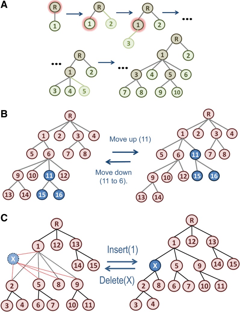
Operations for adding, moving, and deleting nodes. (A) The AddLeaf() operation. This operation is applied to both internal nodes (brown) and existing leaf nodes (green) and can construct a complex hierarchy by repeatedly sampling new leaf nodes. In each step, the resultant hierarchy is subsequently optimized by omcBPPS sampling over sequence assignments and patterns. Nodes selected for spawning off a new leaf node (in the first three steps) are haloed in red. (B) The MoveUp() and MoveDown() operations. The nodes in the subtree being moved are shown in blue. (C) The Insert() and Delete() operations. Insert() adds a new internal node (shown in blue) into an existing hierarchy. Delete() can remove either an internal node (as shown) or a leaf node.

3.2.1. The add leaf operation

The primary operation for creating a hierarchy de novo is AddLeaf(). As illustrated in Figure 2A, AddLeaf() splits off a new leaf node from an existing node. Those sequences that are initially assigned to the existing node are partitioned between the two resultant (parent and child) nodes. This partitioning is performed by sampling, from among the source node sequences, one subset of sequences that are more similar to each other than they are to the remaining sequences associated with the source node. Next, using this starting configuration, BPPS sampling is applied to optimize the sequence partitions and patterns over every contrast alignment for which this new node (designated z′) is assigned to either the foreground or background partition (i.e., ). After sampling a candidate in this way, Metropolis sampling (Hastings, 1970) between the previous versus the new hierarchy is performed. The Delete() sampling operation reverses the AddLeaf() operation by merging a leaf node and its associated sequences into the parent node.

3.2.2. Move up and down operations

The AddLeaf() operation favors the selection of larger subgroups (as new leaf nodes) insofar as these generally correspond to higher LLRs, but it is not guaranteed to do so. Consequently, the hierarchy so obtained may have either misplaced subtrees or missing internal nodes. To optimize the placement of subtrees and nodes, the MoveUp() and MoveDown() operations (which are illustrated in Fig. 2B) move a node from its parent node either up to its grandparent node or down to one of its sibling nodes, respectively. These operations do not change the sequences assigned to the nodes in the repositioned subtree, though it does, of course, change the partition assignments for certain contrast alignments (i.e., the H_h). Thus, after the MoveUp() operation is performed, sequences and patterns are sampled across the new parent (the previous grandparent) subtree before performing a Metropolis step that samples between the initial versus the new hierarchy. For the MoveDown() operation, sequences and patterns are likewise sampled across the new grandparent subtree before the sampling step. Of course, MoveUp() reverses MoveDown() and vice versa.

3.2.3. Insert operation

The Insert() operation (which is illustrated in Fig. 2C) facilitates escape from hierarchies that are suboptimal because of missing internal nodes. It inserts a new node between an existing parent node and two or more (but not all) of its child nodes. The Delete() operation reverses the Insert() operation. For each parent node, the Insert() operation needs to explore every combination of the allowed number of child nodes to attach to the inserted node, such that one out of possible subtrees is sampled, where n is the total number of child nodes. Because this number becomes very large for large n, this procedure can be computationally very intensive. There are, for example, 1,073,741,792 combinations for n = 30 and 1.27 × 10³⁰ for n = 100. Therefore, to sample these possibilities in reasonable time, a branch-and-bound-like (Land and Doig, 1960) recursive procedure is used that prunes regions of the search space that are highly unlikely to yield fruitful configurations. Conceptually, this procedure works by first screening every combination of two child subtrees as the foreground partition and one remaining child subtree as the background partition. Next, using the best of these candidate subcombinations for each child node (and avoiding redundant configurations), it recursively searches deeper. However, at each level of recursion, it only searches deeper for the best combination found at that level and for which every foreground child node has a positive contributions to an approximate contrast alignment LLR computed “on-the-fly.” Finally, it optimizes the best configuration among the (completed) configurations found in this way before Metropolis sampling of the previous versus this proposed hierarchy.

3.3. Data structures

To perform sampling operations efficiently, it is helpful to use a tri-partition table (an H-table) that gives the direct correspondence between the tri-partitions defined by H and the nodes in the hierarchy. The correspondence between a tree and an H-table is shown in Figure 3A,B. An arbitrary tree (having N nodes that have been numbered sequentially via a depth-first search) is converted into an H-table as follows. For each of the 1 ≤ n ≤ N nodes, in the nth column of the table add “+,” “−,” and “o” symbols to those rows corresponding, respectively, to the subtree rooted at the nth node, to the rest of the subtree rooted at the parent of the nth node, and to the remaining (unassigned) nodes. The last row of the table corresponds to a set of random sequences that serves as the parent of the root node. Hence, the nth row of an H-table corresponds to the nth node in the tree and the nth column corresponds to the nth contrast alignment and to the nth tri-partition (i.e., to H_h where h = n).

FIG. 3.

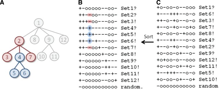
Correspondence between a tree and an H-table. (A) The tree from Figure 1C representing the hierarchical relationships between protein subgroups highlighting the foreground (blue nodes) and background (maroon nodes) nodes for the subtree rooted at node 4. Nonparticipating nodes are shown in gray. (B) The corresponding H-table in standard tree format. Names of leaf and internal nodes are terminated by exclamation and question marks respectively. The node 4 subtree is highlighted in the table to correspond to the tree in (A). (C) A scrambled version of the table shown in (B), which the Sort() operation unscrambles.

This H-table data structure facilitates MoveUp() and MoveDown() operations by simply changing the symbols in the cells of the table. However, this can obscure a table's correspondence to the tree that it represents by permuting the columns and rows. Such scrambled H-tables (like the one shown in Fig. 3C) will still correspond to a tree as long as they satisfy the constraints specified in Equations 8 and 9 above. However, performing other operations efficiently requires that the H-table be in a “standard tree-format,” where each foreground subset (i.e., each ) is to the right of its “ancestral” superset and where each contrast alignment (i.e., subtree) specified by the nth column corresponds to the nth row (i.e., to that subtree's root node) in the table (as in Fig. 3B). The Sort() operation converts tables into the standard format. Note that, for a given hierarchy, typically there are multiple H-table arrangements satisfying this standard format. Likewise, H-table operations are applied to perform the Insert(), Delete(), and AddLeaf() operations described above. For descriptions of other data structures, see Neuwald et al. (2003), Neuwald and Liu (2004), and Neuwald (2011).

3.4. Algorithms

The pseudocode for the AddLeaf() operation follows in Algorithm 1.

Algorithm 1. Algorithm for Adding Leaves
A. Store the current hierarchy's nodes (ordered by decreasing numbers of sequences) on a heap (Tarjan, 1983).
B. While there are nodes associated with at least np sequences on the heap, do
1. Take the largest node off the heap as a potential new parent node.
2. Create a consensus sequence of the associated sequences.
3. Attach a new leaf node to this node.
4. For each of nc randomly sampled sequences associated with the parent node,
a. Partition the parent node sequences based on similarity to the sampled versus the consensus seq.
b. Create a child node consensus sequence based on this initial partition.
c. Repartition parent node sequences based on their similarity to one or the other consensus seq.
d. Compute the optimal pattern distinguishing the child partition from the rest of the parent subtree.
e. Compute the LLR for the corresponding contrast alignment.
5. Sample one of these nc configurations proportional to the associated LLRs, and do the following:
a. Initialize the new leaf node with the sampled pattern and the corresponding partition.
b. Perform BPPS sampling over the parent subtree.
c. Save the optimal configuration found for this modified hierarchy.
6. Sample the resultant hierarchy versus the existing hierarchy (Metropolis et al., 1953).
7. If the new leaf node was sampled, then insert both the new parent and child nodes onto the heap.
C. Return.

The parameter n_c is chosen to be significantly less than the number of sequences associated with the parent node, as this enhances the stochastic nature of the algorithm. I also impose a strict minimum limit of N_L sequences assigned to leaf nodes so that nodes lacking N_L sequence assignments are deleted. Hence, changing these parameters may favor hierarchies with greater or fewer nodes, depending on the level of detail desired for a given protein domain. (By default, n_p = 100, n_c = 40, and N_L = 40.) Alternatively, underlying Bayesian prior probabilities could be adjusted to favor larger or smaller hierarchies, though what sort of node size cutoff this would impose is unclear.

The algorithm for moving a (target) subtree up the hierarchy involves changing the symbols in the H-table, as specified by Algorithm 2. (Moving nodes down in the hierarchy merely reverses this operation and thus is not given here.)

Algorithm 2. Algorithm for Moving Nodes Up the Hierarchy
A. Set the new background partition for the target subtree equal to the grandparent's other descendent nodes.
(Note that the target subtree's foreground does not change.)
B. Set the target subtree foreground sets from the foreground to the background of the old parent node and remove them from the background of the old parent's original descendent nodes.
C. Sample the proposed versus the current hierarchy.
D. If the proposed hierarchy is sampled, sort the H-table data structure to return to standard tree format.

Algorithm 3 inserts (“missing”) internal nodes using a recursive search procedure with pruning (in steps A.2 and A.3.a.ii).

Algorithm 3. Algorithm for Inserting Internal Nodes
A. For each nonroot internal node with at least three child nodes:
1. Create a heap for storing the K best contrast alignments (K = 25 by default).
2. For each child subtree of the selected internal node,
a. Assign the child subtree to the foreground of a contrast alignment.
b. For each combination of two other child subtrees,
i. Assign one of these to the background and the other to the foreground.
ii. Compute the optimal pattern and corresponding likelihood-ratio for this contrast alignment.
iii. Save this configuration and its likelihood-ratio.
c. Sample one of these three-subtree configurations proportional to its likelihood.
d. Put the sampled configuration on the heap using its LLR as the key.
3. For each item on the heap (from the highest to the lowest LLR):
a. Recursive assign the rest of the child subtrees first to the foreground and next the background. At each level of recursion,
i. Compute the optimal pattern and the LLR for the current contrast alignment.
ii. Search deeper only if the LLR contribution of each foreground subtree is positive.
iii. If the configurations are complete at that level, then sample and return one of them.
(“Complete” = all child subtrees have been assigned to either the foreground or background.)
b. Put the sampled configuration so obtained for the current item on a second heap.
4. For each of k (where k < K; by default k = 10) contrast alignments on the second heap (starting with the best),
a. Insert the new internal node into the tree.
b. Assign the child subtrees as specified for the contrast alignment.
b. Sample over the sequences and patterns in the inserted node's subtree.
c. Sample between the best hierarchy found in this way versus the previous hierarchy.
d. If a new hierarchy is sampled, then break out of this (step A.4) subloop.
5. If a new hierarchy was sampled, then break out of this main (step A) loop.
B. If a new hierarchy was sampled, then start over again at step A, otherwise, return.

4. Results

The omcBPPS sampler was implemented in C++ and applied to 60 protein domains to evaluate how well it finds the likely globally optimal peaks in hierarchy space. These domains were selected from the NCBI CDD, and their manually curated hierarchies span a representative range of complexities (Table 1). A multiple-sequence alignment for each domain was obtained as previously described (Neuwald et al., 2012) and used as input to the omcBPPS program. (For biological evaluations of multiple-category BPPS analyses, see Neuwald, 2011.) This output was evaluated with following questions in mind: Does the sampler appear to find the optimal or nearly optimal hierarchy? Does it significantly improve upon the corresponding curated hierarchy? And how similar are independent nearly optimal hierarchies?

Table 1.

Protein-Conserved Domains Used in This Study

Identifier	Description	Length	No. of sequences	LLR (nats)	No. of nodes
cd00004	Sortases	128	2,966	33,467	20
cd00113	PLAT/LH2	116	5,437	68,836	41
cd00121	Meprin and TRAF-C homology	126	3,800	36,081	24
cd00142	PI3Kc_like	219	2,956	52,990	35
cd00159	RhoGAP	169	5,904	96,103	59
cd00173	SH2 domain	79	7,022	60,390	54
cd00203	Zn-dependent metalloprotease	167	8,692	153,246	74
cd00296	SIR2	222	5,347	93,658	55
cd00316	Oxidoreductase_nitrogenase	399	2,923	99,377	45
cd00321	Sulfite oxidase, molybdopterin binding	156	4,109	54,131	35
cd00326	Carbonic anhydrase alpha	227	3,593	56,314	33
cd00413	Glycosyl hydrolase family 16	210	9,324	171,049	74
cd00421	Intradiol dioxygenases	146	2,624	37,774	26
cd00465	URO-D_CIMS_like	306	9,565	272,045	105
cd00516	Phosphoribosyltransferase type II	281	6,514	186,731	75
cd00518	Hydrogen maturation proteases	139	1,386	12,156	13
cd00538	Protease-associated (PA)	126	7,602	105,141	67
cd00596	Peptidase_M14_like	211	7,856	190,121	77
cd00599	Endo-N-acetylmuramidases	186	3,286	60,163	34
cd00688	ISOPREN_C2_like	300	3,919	107,289	41
cd01060	Membrane fatty acid desaturase-like	122	9,624	141,359	73
cd01067	Globin_like	117	11,420	223,561	107
cd01081	Aldose 1-epimerases or mutarotases	284	6,431	169,420	64
cd01363	Myosin and kinesin motors	186	9,992	120,733	76
cd01819	Patatin-like phospholipase	155	8,728	123,798	75
cd01951	Legume-type lectins	223	3,361	57,645	39
cd02257	Peptidase C19	255	6,405	142,178	66
cd02742	GH20_hexosaminidase	303	2,943	73,198	34
cd02749	Macro domain	147	4,200	42,989	28
cd02775	Molybdopterin-binding, C-terminal	101	9,289	142,616	82
cd03523	NTR_like	105	1,421	11,241	14
cd04369	Bromodomain	99	7,016	48,764	42
cd04370	Bromo adjacent homology	123	2,784	34,138	23
cd04371	DEP domain	81	1,777	14,203	20
cd04519	RasGAP	318	1,170	23,607	17
cd04748	COMM domain	87	1,369	7,732	12
cd05119	RIO kinase family, catalytic domain	187	2,784	33,426	27
cd05396	Animal heme peroxidase like	370	1,455	37,156	18
cd05467	Family 20 carbohydrate-binding module	96	1,721	9,937	11
cd05992	PB1 domain	81	4,634	40,615	33
cd06099	CS_ACL-C_CCL domain	213	8,375	73,635	48
cd06157	Ligand-binding domain of nuclear receptor	168	4,043	70,898	52
cd06169	Bacterial micro-compartment (BMC)	62	2,333	12,202	18
cd06589	Glycosyl hydrolase family 31	265	3,273	76,405	35
cd06663	Biotinyl-lipoyl	73	29,455	128,216	68
cd06846	Adenylation_DNA_ligase_like	182	4,943	81,717	44
cd07320	Extradiol_Dioxygenase_3B_like	260	3,882	81,701	36
cd07323	La motif RNA-binding	75	2,548	11,918	11
cd07440	Regulator of G-protein signaling (RGS)	113	2,922	26,904	22
cd07954	AP_MHD_Cterm	239	3,208	66,503	31
cd08150	catalase_like	283	4,311	60,978	39
cd08304	Death domain (DD) superfamily	69	5,204	22,428	36
cd08555	PI-PLCc_GDPD_SF	179	11,186	272,789	105
cd08772	GH43_62_32_68 (β propellers)	286	8,623	283,306	94
cd08773	FpgNei_N domain	117	4,820	36,212	28
cd08961	Glycoside hydrolase family 64 and thaumatin-like	153	9,250	63,068	46
cd09487	Sterile alpha motif	56	8,030	53,463	67
cd09593	Uracil-DNA glycosylase like	125	9,099	113,842	53
cd10148	CsoR-like_DUF156	80	2,180	10,593	14
cd10785	GH38-57_N_LamB_YdjC_SF	203	6,085	143,340	62

The first column gives the National Center for Biotechnology Information's Conserved Domain Database identifiers for each domain. The LLR and the number of nodes correspond to the optimal hierarchy found among the three starting points. LLR, log-likelihood ratio.

4.1. Evidence that the sampler typically finds a nearly optimal hierarchy

The sampler's ability to find an optimal or nearly optimal hierarchy was tested by determining whether it consistently finds the same or nearly the same hierarchy using three independent starting points, namely, (i) a single root node, that is de novo; (ii) a hierarchy that was generated heuristically (Neuwald et al., 2012); and (iii) a manually curated hierarchy obtained from the NCBI's CDD (version 3.09). For each starting point, three processes were run in parallel and the highest scoring hierarchy was retained. This analysis was run several times with very similar results. The results of one such analysis are summarized in Figure 4. The run times varied from about 8 minutes to several days depending on the size and length of the input alignment (given in Table 1) and on the number of subgroups.

FIG. 4.

(A) Plot of hierarchy LLRs for the 60 domains listed in Table 1. Hierarchies were created by the omcBPPS sampler initialized from three different starting points: de novo, □; from a hierarchy created heuristically (Neuwald et al., 2012), ◯; and from a manually curated CDD hierarchy, △. The line corresponds to the average for the three methods. (B) Plot of the numbers of nodes obtained for each hierarchy. A scatter plot (inset) of the RSD for the LLR versus the RSD for the numbers of nodes reveals an outlier (top right corner) corresponding to cd08304. CDD, Conserved Domain Database; LLRs, log-likelihood ratios; omcBPPS, optimal multiple-category BPPS; RSD, relative standard deviation.

The plot in Figure 4A reveals that, when initiated from any of the three starting points, the sampler typically converges on hierarchies with very similar LLRs. The three LLRs exhibited an average relative standard deviation (RSD) of 1.7% (over the 60 domains). This variability is fairly consistent as it is similar for the 30 domains with lowest versus the highest LLRs, namely, 2.3% versus 1.0%—though the latter is somewhat less variable. Greater variability is observed in the number of nodes obtained for the three runs: the plot in Figure 4B indicates an RSD of 5.1% when averaged over the 60 domains. Again, this variability is fairly consistent between the 30 smallest and 30 largest hierarchies, namely, 6.8% and 3.4%, respectively—though again the larger domains show less relative variability. Thus, the variability fails to scale up in line with increased size or LLR of a hierarchy. The slightly greater variability associated with hierarchy size versus LLR suggests that the optimal peak in the posterior probability distribution for the average domain may consist of an ensemble of slightly different hierarchies. Such differences between independently generated hierarchies are examined in detail in the following sections.

The choice of starting hierarchy typically has no significant influence on the outcome. That is, there is no overall advantage in choosing one starting hierarchy over another. This was determined by computing, for each of the three starting hierarchies used in the analysis, the binomial tail probability:

where x is the observed number of “successes” in n = 60 trials and where each of the three starting hierarchies are taken as equally likely to succeed (i.e., q = ⅓). When success is defined as obtaining the highest LLR among the three for one of the starting points, the resulting p-value, in each case, was insignificant:p ≥ 0.34 (unadjusted for multiple hypotheses). Redefining success as the lowest LLR was likewise insignificant: p ≥ 0.65. The type of starting hierarchy similarly failed to significantly increase or decrease the size of the final hierarchy: p ≥ 0.32 and p ≥ 0.78, respectively. Taken together, these results indicate that, regardless of the starting point, the sampler typically converges on a similarly optimal peak in the posterior probability distribution.

The inset in Figure 4B reveals one outlier, however, the Death domain (cd08304), for which the RSDs over the LLR and the numbers of nodes were 12.2% and 26.5%, respectively. This appears because of the curated hierarchy (which was used as one of the starting points) being exceptionally poor; it consists of 81 nodes, 60 nodes of which were rejected by the sampler during optimization. Moreover, this curated hierarchy bears no obvious resemblance to the optimal hierarchy found, which consists of 36 nodes. This suggests that, when starting from a strikingly suboptimal starting point, the sampler may fail to find the global optimum.

4.2. Improving a manually curated hierarchy

Comparing an optimized hierarchy with a manually curated hierarchy is complicated by the variable criteria used by curators. For example, one curator may require each subgroup in a hierarchy to correspond to proteins with a fairly high degree of taxonomic or sequence diversity, whereas another curator may favor splitting up a hierarchy into less diverse subgroups. These two approaches will result in hierarchies with fewer or greater numbers of nodes, respectively. Although the omcBPPS sampler parameter settings can be modified in a similar manner, precisely how to match the (undefined and possibly inconsistent) criteria used by each curator is unclear. Moreover, CDD hierarchies are typically in various stages of manual curation, and thus many of these are incomplete.

As an alternative to direct comparisons, I examined the contributions of individual nodes to the LLR at various levels of either the curated or the sampler-optimized hierarchy. (Sequence and pattern assignments for each curated hierarchy were optimized via sampling although without modifying the hierarchy or the curator-assigned seed sequences for each node.) Figure 5 shows one such comparison for a recent (prerelease) CDD hierarchy for globin-like domains (cd01067). This reveals that individual nodes contributing to the second level of the curated hierarchy provide, on average, 516 nats to this aspect of the hierarchy's LLR (of 126,945 nats). However, nearly half of this is because of a single node (cd12127), with most of the other nodes having either small or negative contributions (Fig. 5A). The corresponding nodes for the sampler optimized hierarchy (Fig. 5B) all contribute positively and, on average, nearly 2½ times more (1,263 nats) to this aspect of the LLR (of 223,561 nats). Notably, all three sampler-optimized hierarchies are very similar (see Supplementary Fig. S1; Supplementary Material is available online at www.liebertpub.com/cmb), supporting the notion that the sampler has found a nearly optimal hierarchy.

FIG. 5.

Contributions of individual nodes to the second level of the curated versus optimal hierarchies for globin-like domains (cd01067). Nodes shown in green and red contribute (positively or negatively, respectively) to the LLR at the second or lower levels of the hierarchy, as plotted below each hierarchy. Other nodes are shown in blue. (A) Manually curated hierarchy (LLR score: 126,945 nats; 43 nodes). Numbers are labeled with their CD identifiers. (B) Optimized hierarchy obtained using the curated CDD hierarchy as a starting point (223,561 nats; 55 nodes).

4.3. Example of a robust hierarchy

Because sampling occurs stochastically, distinct random seeds or starting configurations will lead to distinct sampling pathways, which is useful for assessing the robustness of a hierarchy by determining whether the sampler generally finds very similar hierarchies from different starting points. For some domains, the sampler converges on nearly identical hierarchies, as is seen for oxidoreductase/nitrogenase domains (cd00316) in Figure 6A–C. All of the nodes in each hierarchy correspond to nodes in at least one, and in nearly all cases both, of the other hierarchies. Likewise, all of the nodes in the manually curated hierarchy (Fig. 6D) correspond to nodes in the optimal hierarchy (Fig. 6E). Although the optimal hierarchy contains additional nodes, this mainly appears because of the use of different criteria by this particular curator versus the sampler, which has further subclassified the major subgroups. The sampler converges on similarly robust hierarchies for other domains, including, for example, the globin-like domains (see Supplementary Fig. S1), for which, however, there is less agreement with the curated hierarchy (Supplementary Fig. S2). Three moderately robust hierarchies for the SIR2 domain (cd00296) are shown in Supplementary Figure S3. In such cases, constructing a consensus hierarchy from several of these hierarchies is feasible.

FIG. 6.

Example of a robust hierarchy; the oxidoreductase/nitrogenase domain (cd00316). (A) Hierarchy generated de novo (96,708 nats; 43 nodes). (B) Hierarchy obtained using the curated CDD hierarchy as a starting point (99,377 nats; 45 nodes). The correspondence between nodes of the hierarchies in (A) and in (C) to nodes in the hierarchy in (B) is indicated using the color code defined in the box. (C) Hierarchy obtained using a heuristic hierarchy as the starting point (98,708 nats; 46 nodes). (D) The CDD manually curated hierarchy (71482 nats; 16 nodes). (E) The hierarchy shown in (B) but re-colored for comparison with the NCBI manually curated hierarchy in (D). The light-red nodes are nodes that fail to correspond to a node in (D) and that are less diverse than the least diverse node in (D). Numbers in parentheses correspond to the number of phyla represented by the sequences assigned to those nodes. For comparison, the nodes in the manually curated hierarchy all have sequences from at least four phyla. NCBI, National Center for Biotechnology Information.

4.4. Example of a challenging hierarchy

For other domains, however, the nature of the hierarchy optimized by the sampler varies depending on the starting hierarchy or on the random seed. Figure 7 shows one such example, the catalytic domain of phosphoinositide 3-kinase (PI3Kc)-like proteins (cd00142). Most of the nodes (about 80–85%) in one hierarchy correspond to nodes in another, independently optimized hierarchy (i.e., each share ≥90% of assigned sequences) or else roughly correspond (i.e., each share >50% of assigned sequences). There are, however, significant differences. These differences seem unlikely to reflect a failure to find the optimal or nearly optimal hierarchy for two reasons. First, the LLR for all three hierarchies is nearly the same: on average, the values differ from the mean by less than 1%. Second, the contributions of each node to the LLR at each level of each hierarchy are positive and nearly always at least 100 nats, thereby supporting each of the alternative hierarchies. In part, such discrepancies between hierarchies are caused by some of the leaf nodes barely meeting the minimal criteria used by the sampler for detection; thus, these are modeled inconsistently. However, there are other well-supported nodes that are also inconsistently modeled. Why then do these differences occur?

FIG. 7.

Comparison of the hierarchies obtained for the catalytic domain of phosphoinositide 3-kinase (PI3Kc)-like proteins. (A) Hierarchy obtained using the curated CDD hierarchy (cd00142) as a starting point (51,784 nats; 33 nodes). Node numbering likewise corresponds to the node numbering in (B). (B) A hierarchy generated de novo (52,990 nats; 36 nodes). (C) Optimal hierarchy obtained using a heuristic hierarchy as the starting point (52,650 nats; 36 nodes).

One explanation is that these alternative trees reflect complex patterns of conserved residues and corresponding properties that cannot be modeled by a single hierarchy, as is illustrated hypothetically in Figure 8. This can occur when subsets of proteins from different clades share certain biochemical properties, presumably inherited from an ancestor of both clades, but lost in some but not all members of each clade because of a relaxation of selective constraints upon those other members. This has been confirmed, for example, for divergent eukaryotic Replication Factor C DNA clamp loader AAA+ subunits (Neuwald, 2011). The fact that for other domains (as in Fig. 6) the sampler consistently converges on essentially the same hierarchy further supports the notion that significant differences between nearly optimal hierarchies may be because of complex patterns of conserved residues (and presumably of underlying conserved biochemical properties) that cannot be modeled by a single hierarchy.

FIG. 8.

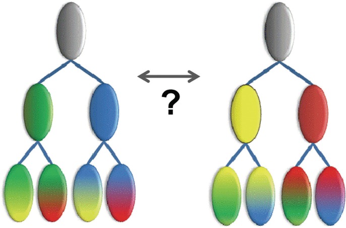
Hypothetical illustration of patterns inconsistent with a single tree. The same four leaf nodes, each of which harbor two out of four properties (green, yellow, blue, and red), may be arranged in two different ways, where, for each tree, intermediate nodes model only one of the conserved properties.

5. Discussion and Conclusion

The omcBPPS sampler differs from existing protein classification methods that cluster sequences either based on pairwise similarity (Remm et al., 2001; Abascal and Valencia, 2002; Li and Godzik, 2006) or by cutting phylogenetic trees (Wicker et al., 2001; Storm and Sonnhammer, 2002; Zmasek and Eddy, 2002; Engelhardt et al., 2011), which are also constructed based on sequence similarity scores. Condensing detailed similarities and differences between sequences into single overall alignment scores in this way discards valuable biological information. The omcBPPS sampler retains this information by classifying sequences through explicit modeling of divergent residue signatures. Unlike other methods, the omcBPPS sampler focuses on constructing a hierarchy of domain subgroups for a specific protein class.

This has obvious application in automated generation and optimization of protein domain hierarchies, as for the NCBI CDD. Moreover, the sampler automatically generates subgroup alignments both for leaf nodes, which correspond to fully differentiated sequence subgroups, and for intermediate nodes, which correspond to undifferentiated sequences that conserve patterns common to that node's subtree but that lack patterns specific to descendant nodes. This provides a mechanism to ensure appropriate coverage of protein domain subgroups, which is an aim of the PFAM protein domain database (Finn et al., 2008). Both databases currently rely on manual curation for these algorithmically challenging tasks, which the omcBPPS sampler now accomplishes automatically.

Because a protein class can consist of tens of thousands of sequences, modeling evolutionary divergence hierarchically in this way is more tractable and interpretable than constructing extremely large phylogenetic trees. It also provides additional evolutionary perspectives. For long domains within a large and functionally diverse protein class, such as the eukaryotic protein kinases, however, the sampler currently requires considerable time for optimization. Thus, further algorithmic and strategic improvements are needed, such as perhaps first optimizing over only the major subgroups followed by modeling each major subtree in more detail one-at-a-time. A faster version of the sampler will facilitate other applications, such as computing the predictive probability of membership for each sequence within each subgroup and estimation of confidence levels for individual nodes within a hierarchy.

The analysis here indicates that the sampler consistently finds statistically optimal or nearly optimal hierarchies for a wide variety of domains. It thus constitutes an algorithmic solution to the problem of finding an optimum protein domain hierarchy consisting of clusters of functionally divergent subgroups. For some domains, however, a single optimal or nearly optimal hierarchy appears to be replaced by an ensemble of slightly different hierarchies. In some cases, these may be because of evolutionary events that defy preconceived notions and thus are inconsistent with a single phylogenetic tree. In a companion article (Neuwald, 2013), I explore this phenomenon and other aspects of domain hierarchies in greater detail.

Acknowledgments

This work was supported by the School of Medicine at the University of Maryland, Baltimore, and by NIH contract HHSN2630000999571.

Author Disclosure Statement

No competing financial interests exist.

References

- Abascal F., and Valencia A.2002. Clustering of proximal sequence space for the identification of protein families. Bioinformatics 18, 908–921 [DOI] [PubMed] [Google Scholar]
- Engelhardt B.E., Jordan M.I., Srouji J.R., et al. 2011. Genome-scale phylogenetic function annotation of large and diverse protein families. Genome Res. 21, 1969–1980 [DOI] [PMC free article] [PubMed] [Google Scholar]
- Finn R.D., Tate J., Mistry J., et al. 2008. The Pfam protein families database. Nucleic Acids Res. 36, D281–D288 [DOI] [PMC free article] [PubMed] [Google Scholar]
- Hastings W.K.1970. Monte Carlo sampling methods using Markov Chains and their applications. Biometrika 57, 97–109 [Google Scholar]
- Kirkpatrick S., Gelatt C.D., and Vecchi M.P.1983. Optimization by simulated annealing. Science 220, 671–680 [DOI] [PubMed] [Google Scholar]
- Land A.H., and Doig A.G.1960. An automatic method of solving discrete programming problems. Econometrica 28, 497–520 [Google Scholar]
- Li W., and Godzik A.2006. Cd-hit: a fast program for clustering and comparing large sets of protein or nucleotide sequences. Bioinformatics 22, 1658–1659 [DOI] [PubMed] [Google Scholar]
- Liu J.S.2008. Monte Carlo Strategies in Scientific Computing. Springer-Verlag, New York [Google Scholar]
- Marchler-Bauer A., Lu S., Anderson J.B., et al. 2011. CDD: a Conserved Domain Database for the functional annotation of proteins. Nucleic Acids Res. 39, D225–D229 [DOI] [PMC free article] [PubMed] [Google Scholar]
- Metropolis N., Rosenbluth A.W., Rosenbluth M.N., et al. 1953. Equations of state calculations by fast computing machines. J. Chem. Phys. 21, 1087–1092 [Google Scholar]
- Neuwald A.F.2011. Surveying the manifold divergence of an entire protein class for statistical clues to underlying biochemical mechanisms. Stat. Appl. Genet. Mol. Biol. 10, 36. [DOI] [PMC free article] [PubMed] [Google Scholar]
- Neuwald A.F.2013. Evaluating, comparing and interpreting protein domain hierarchies. J. Comp. Biol. (in press). [DOI] [PMC free article] [PubMed] [Google Scholar]
- Neuwald A.F., and Liu J.S.2004. Gapped alignment of protein sequence motifs through Monte Carlo optimization of a hidden Markov model. BMC Bioinform. 5, 157. [DOI] [PMC free article] [PubMed] [Google Scholar]
- Neuwald A.F., Kannan N., Poleksic A., et al. 2003. Ran's C-terminal, basic patch and nucleotide exchange mechanisms in light of a canonical structure for Rab, Rho, Ras and Ran GTPases. Genome Res. 13, 673–692 [DOI] [PMC free article] [PubMed] [Google Scholar]
- Neuwald A.F., Lanczycki C.J., and Marchler-Bauer A.2012. Automated hierarchical classification of protein domain subfamilies based on functionally-divergent residue signatures. BMC Bioinform. 13, 144. [DOI] [PMC free article] [PubMed] [Google Scholar]
- Remm M., Storm C.E., and Sonnhammer E.L.2001. Automatic clustering of orthologs and in-paralogs from pairwise species comparisons. J. Mol. Biol. 314, 1041–1052 [DOI] [PubMed] [Google Scholar]
- Sayers E.W., Barrett T., Benson D.A., et al. 2011. Database resources of the National Center for Biotechnology Information. Nucleic Acids Res. 39, D38–D51 [DOI] [PMC free article] [PubMed] [Google Scholar]
- Storm C.E., and Sonnhammer E.L.2002. Automated ortholog inference from phylogenetic trees and calculation of orthology reliability. Bioinformatics 18, 92–99 [DOI] [PubMed] [Google Scholar]
- Tarjan R.E.1983. Data Structures and Network Algorithms, 85–96 Society for Industrial Mathematics, Philadelphia [Google Scholar]
- Wicker N., Perrin G.R., Thierry J.C., et al. 2001. Secator: a program for inferring protein subfamilies from phylogenetic trees. Mol. Biol. Evol. 18, 1435–1441 [DOI] [PubMed] [Google Scholar]
- Zmasek C.M., and Eddy S.R.2002. RIO: analyzing proteomes by automated phylogenomics using resampled inference of orthologs. BMC Bioinform. 3, 14. [DOI] [PMC free article] [PubMed] [Google Scholar]
Associated Data
This section collects any data citations, data availability statements, or supplementary materials included in this article.