

Abstract
At one level of abstraction neural tissue can be regarded as a medium for turning local synaptic activity into output signals that propagate over large distances via axons to generate further synaptic activity that can cause reverberant activity in networks that possess a mixture of excitatory and inhibitory connections. This output is often taken to be a firing rate, and the mathematical form for the evolution equation of activity depends upon a spatial convolution of this rate with a fixed anatomical connectivity pattern. Such formulations often neglect the metabolic processes that would ultimately limit synaptic activity. Here we reinstate such a process, in the spirit of an original prescription by Wilson and Cowan (Biophys J 12:1–24, 1972), using a term that multiplies the usual spatial convolution with a moving time average of local activity over some refractory time-scale. This modulation can substantially affect network behaviour, and in particular give rise to periodic travelling waves in a purely excitatory network (with exponentially decaying anatomical connectivity), which in the absence of refractoriness would only support travelling fronts. We construct these solutions numerically as stationary periodic solutions in a co-moving frame (of both an equivalent delay differential model as well as the original delay integro-differential model). Continuation methods are used to obtain the dispersion curve for periodic travelling waves (speed as a function of period), and found to be reminiscent of those for spatially extended models of excitable tissue. A kinematic analysis (based on the dispersion curve) predicts the onset of wave instabilities, which are confirmed numerically.
Electronic supplementary material
The online version of this article (doi:10.1007/s00285-013-0670-x) contains supplementary material, which is available to authorized users.
Keywords: Neural field models, Travelling waves, Refractoriness, Delay differential equations
Introduction
The continuum approximation of neural activity can be traced back to work of Beurle (1956), who built a model describing the proportion of active neurons per unit time in a given volume of randomly connected nervous tissue. A major limitation of this very early neural field model is its neglect of refractoriness or any process to mimic the metabolic restrictions placed on maintaining repetitive activity. It was Wilson and Cowan (1972, 1973) who first developed neural field models with some notion of refractoriness. At the same time they also emphasised the importance of modelling neural population in terms of an excitatory subpopulation and an inhibitory subpopulation. Indeed over the years many studies of the Wilson-Cowan excitatory-inhibitory model have been made, with applications to problems in neuroscience ranging from the generation of electroencephalogram rhythms through to visual hallucinations, and see (Coombes et al. 2003) for a review. However, many of these subsequent studies drop the refractory term and focus more on the role of excitatory-inhibitory interactions in generating neural dynamics. Perhaps one exception to this is the work of Curtu and Ermentrout (2001), who have shown that the original Wilson-Cowan model with refractoriness can drive oscillations even in the absence of inhibition. Their work was done for a point model which begs the question as to whether refractoriness alone can allow for periodic waves to be generated in a spatially extended excitatory network. This is an especially intriguing issue given that neural field models with some form of inhibition or negative feedback, such as spike frequency adaptation, have traditionally been invoked to explain wave behaviour in cortex, including fronts, pulses, target waves and spirals (Ermentrout and McLeod 1993; Pinto and Ermentrout 2001; Huang et al. 2004).
In this paper we reinstate the original refractory term of Wilson and Cowan in a minimal neural field model describing a single population in one spatial dimension. This model is briefly reviewed in Sect. 2. In Sect. 3 we present a linear stability analysis, as well as a weakly nonlinear analysis, of the homogeneous steady state that predicts the onset of periodic travelling wave patterns in a purely excitatory network. This is confirmed by direct numerical simulations that show periodic travelling waves with profiles that appear as either single or multiple spikes of activity. A novel numerical continuation scheme is developed to track solution properties in a co-moving frame (speed, period, and profile shape) as a function of physiologically important system parameters (such as refractory time-scale, strength of anatomical connectivity, and firing threshold). These are obtained after recognising that the original model can be reformulated as a delay-differential equation for an exponentially decaying choice of anatomical weight distribution. The delay is set by the time-scale of the refractory process. In Sect. 4 we numerically construct the wave speed as a function of the wave period, to obtain the so-called dispersion curve. Here we avoid special case choices of the weight distribution and develop a numerical scheme that can handle the original delayed integro-differential model. The dispersion curve for an excitatory network with an exponentially decaying weight distribution is shown to have a shape reminiscent of that seen in the study of nonlinear reaction-diffusion systems, and in particular those arising in the study of an axon or active dendrite (Miller and Rinzel 1981). Using the dispersion curve we further develop a kinematic model that allows predictions about non-regular spike trains to be made, including period-doubling scenarios subsequently confirmed by direct numerical simulations. In addition, we establish an example of a homoclinic orbit of chaotic saddle-focus type in an infinite-dimensional system. Finally in Sect. 5 we present a brief discussion of the work in this paper.
The Wilson-Cowan model with refractoriness
Wilson and Cowan considered the spatio-temporal evolution of the activity of synaptically interacting excitatory and inhibitory neural sub-populations (Wilson and Cowan 1972). A recent review of their model can be found in (Coombes et al. 2013; Bressloff 2012). A common reduction of their original model, and one often employed as a minimal model of cortex, takes the form of a scalar integro-differential equation:
 |
1 |
Here  is a temporal coarse-grained variable describing the proportion of neural cells firing per unit time at position
  at the instant
  . The symbol
  represents spatial convolution, the function
  describes an effective anatomical connectivity or weight distribution and is a function of the distance between two points, and
  is the relaxation time-scale. The nonlinear function
  describes the expected proportion of neurons receiving at least threshold excitation per unit time, and is often taken to have a sigmoidal form. In major contrast to the original Wilson-Cowan equations refractory terms are not included in this model. To reinstate such terms in (1) we follow (Wilson and Cowan 1972), and more recently (Curtu and Ermentrout 2001), and model the fraction of cells in their absolute refractory period
  by
by
 |
2 |
Since only a fraction  of cells can be activated and actually contribute to any firing activity the model (1) is modified to
 |
3 |
For convenience we rescale time  and define
  to obtain the model that we shall work with for the remainder of this paper:
 |
4 |
As a choice of firing rate we shall take the sigmoid
 |
5 |
with threshold  and steepness parameter
  . For the choice of weight distribution we shall consider symmetric normalised kernels such that
  and
and  .
.
Analysis of waves
Direct numerical simulations of a purely excitatory network, see below, show the possibility of periodic travelling waves. This is particularly interesting because these are not typically found in neural field models with pure excitation, though they are often encountered in the presence of some form of negative feedback, such as may arise with the inclusion of an inhibitory sub-population or a form of spike frequency adaptation, as reviewed in (Ermentrout 1998). If these patterns arise via the instability of the homogeneous steady state, then they can be predicted using a classic Turing instability analysis. Their analysis beyond the point of instability can be pursued with a weakly nonlinear analysis, to develop a set of amplitude equations (typically in the form of coupled complex Ginzburg-Landau equations), as in (Curtu and Ermentrout 2004; Venkov et al. 2007). However, this is only relevant close to the bifurcation point, and it is much more informative to gain an insight into the fully nonlinear properties of waves using numerical analysis. This has been pursued at length for many excitable systems, and especially for single neuron models of the axon or active dendrite with single (Miller and Rinzel 1981; Röder et al. 2007) or multi-pulse (Evans et al. 1982; Feroe 1982; Hastings 1982; Kuznetsov 1994; Lord and Coombes 2002) periodic waves. However, the study of periodic travelling waves has largely been ignored in the neural field community, which is surprising since this can inform a kinematic analysis [elegantly reviewed in (Keener and Sneyd 1998)] to predict instabilities to more exotic classes of travelling wave solution. We build on a Turing analysis and develop precisely this approach below.
Linear stability analysis of homogeneous solutions
A homogeneous fixed point with  is given by the solution of the nonlinear algebraic equation
 |
6 |
The model displays up to three different fixed points depending on  and
and  , see Fig. 1, which we denote by
  with
with  when three fixed points exist.
Fig. 1.
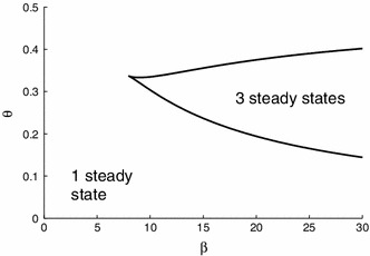
The boundaries in the  -plane with 3 fixed points
Linearising around  and considering perturbations of the form
  gives a dispersion relation for the pair
  in the form
  , where
 |
7 |
 |
8 |
The Turing bifurcation point is defined by the smallest non-zero wave number  that satisfies
  . It is said to be static if
  and dynamic if
  . A static bifurcation may then be identified with the tangential intersection of
  and
and  at
at  . Similarly a dynamic bifurcation is identified with a tangential intersection with
  . Beyond a dynamic instability one would expect the emergence of a periodic travelling wave of the form
  (with speed
  ).
).
For the sigmoidal function (5) we have that  . For an exponential kernel
  , with
  , then
  , which has a maximum of one at the origin. Hence for
  we have that
  where
where
 |
9 |
For large  we see that
  is a decreasing function of
  so that a fixed point will be stable (to a static instability with
  ) if
) if  , or equivalently,
  where
where
 |
10 |
For  it is natural to write
  and equate real and imaginary parts of (7) to obtain two equations for
  and
and  , which we write in the form
 |
11 |
The simultaneous solution of these two equations gives the pair  . For
. For  the above pair of equations reduces to
 |
12 |
Since there are singularities at  , these equations define a series of parametric curves
  defined in the regions
  for
for  . We see that there will be a solution if and only if
 |
13 |
It is clear that (13) defines a quadratic function in  and it turns out that
  does not exist, only
  and
and  . In Fig. 2 we show only the branches with
  as we did not find any with larger
  . Using the observation that
  and
and  we see that a solution for
  is only possible if
  and
and  . Hence a dynamic instability will occur before a static instability when
  and
and  is sufficiently large. To determine whether the static instability gives rise to a travelling or a standing wave it is useful to perform a weakly nonlinear analysis.
Fig. 2.
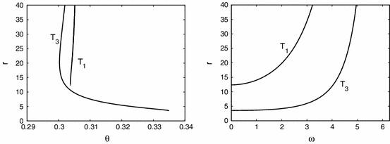
The dependence of the Turing curves  on
on  and
and  with corresponding
  . The
. The  curve corresponds to the lower fixed point,
  corresponds to the higher fixed point. Other parameters are
Weakly nonlinear analysis: amplitude equations
A characteristic feature of the dynamics of systems beyond an instability is the slow growth of the dominant eigenmode, giving rise to the notion of a separation of scales. This observation is key in deriving the so-called amplitude equations. In this approach information about the short-term behaviour of the system is discarded in favour of a description on some appropriately identified slow time-scale. By Taylor-expansion of the dispersion curve near its maximum one expects the scalings  , close to bifurcation, where
  is the bifurcation parameter. Since the eigenvectors at the point of instability are of the type
  , for
, for  emergent patterns are described by an infinite sum of unstable modes (in a continuous band) of the form
  . Let us denote
  where
where  is arbitrary and
  is a measure of the distance from the bifurcation point. Then, for small
  we can separate the dynamics into fast eigen-oscillations
  , and slow modulations of the form
  . If we set as further independent variables
  for the modulation time-scale and
  for the long-wavelength spatial scale (at which the interactions between excited nearby modes become important) we may write the weakly nonlinear solution as
  . It is known from the standard theory (Hoyle 2006) that weakly nonlinear solutions will exist in the form of either travelling waves (TWs),
  or
or  , or standing waves (SWs),
  . In the Appendix we show that (ignoring spatial variation) the amplitude equations take the form
 |
14 |
 |
15 |
where  and
and  are known functions of system parameters. A linear stability analysis of the above amplitude equations generates the conditions for selection between TWs or SWs. If
  and
and  have opposite sign, then a TW exists and for
  and
and  it is stable. If
  and
and  have opposite sign, then a SW exists and for
  and
and  it is stable. Evaluation of the coefficients
  and
and  (see Appendix), yields
  and
and  . Therefore, for typical parameter values the Turing instability is subcritical and travelling and standing waves are unstable. Also, along
  , waves exist for
  if
if  and for
  if
if  . Still, these can be used to start to track waves numerically. Note that a similar weakly nonlinear analysis for waves in a neural field model without refractoriness though with adaptation has been performed in (Curtu and Ermentrout 2004), and for axonal delays in (Venkov et al. 2007).
In the next part we will consider waves and how these can grow beyond a dynamic Turing bifurcation.
Excitability and waves
From the Turing analysis above we expect to see travelling waves for sufficiently large  and suitable
  . A similar observation, based on the numerical simulation of a lattice model with nearest-neighbour coupling has previously been made by Curtu and Ermentrout (2001). These authors further point out that for some range of
  values that the point version of the model (obtained with the choice
  ) can be viewed as an excitable system. The excitability is easily recognised if we consider the spatially homogeneous system
  , with
  and
and  . This can be re-written in delay-differential form as
 |
16 |
We graph the nullcline of the  -equation
  together with the steady states constraint
  and two trajectories in Fig. 3. These show that if an initial displacement from the steady state is sufficiently large, then the trajectory makes a large excursion. In other words, the system is excitable.
Fig. 3.
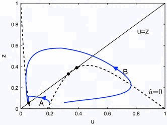
The dashed line indicates the  -nullcline
  with
with  . The steady condition
  (solid black line) intersects the nullcline at 3 points indicated by circles. The trajectories (blue) start from (A)
  and (B)
  and history
  for
for  , i.e. they have been given an initial kick. They approach the lower steady state at
  (colour figure online)
Next we want to show travelling waves for the full spatially extended system defined by (4) using direct numerical simulations. We evolve the state as follows. We use an equidistant spatial discretisation with  mesh points with periodic boundary conditions. We compute the spatial convolution using Fourier transforms. The history integral
  is calculated using a trapezoidal rule with
  points. This gives a system that can be simulated with matlab’s dde23-solver. Supplying the history as
  we obtain a travelling wave, see Fig. 4 (left). Other initial history can also lead to travelling waves as long as the amplitude at one spot is sufficient to cause excitation of neighbouring tissue and the initial spot decays due to refractoriness. The figure suggests that there is enough space to fit in a second moving pulse and this is indeed possible, see Fig. 4 (right). Note that the time from the one pulse to the next is different than from the previous pulse. The travelling waves shown in Fig. 4 have nearly the same velocities namely
  for the travelling one pulse, and
  for the two pulses. The trajectories near the steady state in Fig. 3 also go some way to explaining why the two pulses can move slightly faster. For two pulses in one periodic domain the next pulse arrives when the system is less refractory, i.e.
  is lower, than with only one pulse. We study the dependence of the speed on the wavenumber below.
Fig. 4.
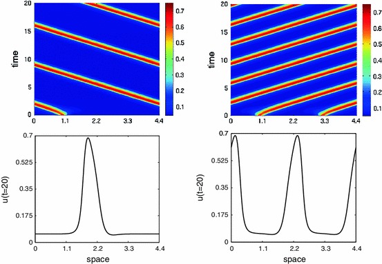
Left a left travelling wave for (4). Right a right travelling 2 pulse wave. The patterns seem to settle after a transient time around  . The lower figures show the profile of the solution
  at
at  . Parameters are
  (colour figure online)
If the domain for the wave becomes infinite, the travelling wave approaches a pulse which is a homoclinic orbit. The linear stability of the steady state in the moving frame  classifies the homoclinic orbit. All travelling waves profiles can be constructed as stationary profiles of (4) in the travelling frame
  , namely as solutions of the dynamical system:
 |
17 |
Focusing now on the homoclinic orbit we consider small perturbations  to obtain
 |
18 |
This has solutions of the form  where
where  is a solution of the transcendental equation
 |
19 |
Here we impose the condition  to ensure convergence of the integral over
  in (18). Fortunately, this includes the imaginary axis allowing stability analysis. If
  we recover the formula derived in (Curtu and Ermentrout 2001) for the Hopf bifurcation of the point model. Solving for the (single) steady state we find
  . We insert the wavespeed
  as observed in the simulations and numerically solve the eigenvalue equation (19) for many random starting values near the origin in the complex plane, see Fig. 5. We find a single positive real eigenvalue
  and the other eigenvalues are complex pairs with negative real part. The leading stable eigenvalues are
  (and satisfy the constraint
  ). We conclude that
  is a saddle-focus with saddle-quantity
  . This implies the existence of N-homoclinic loops for all
  . In particular, we may expect that travelling waves with 3 pulses form an isolated branch and have a saddle-node bifurcation (Gonchenko et al. 1997), even though the system is infinite-dimensional. It is an open challenge to rigorously prove this (and extend the result from the finite dimensional setting). However, it is likely that Lin’s method can be applied in this case, along the lines considered in (Lin 1990) for analysing the bifurcation of a unique periodic orbit from a homoclinic orbit to an equilibrium in a DDE.
Fig. 5.
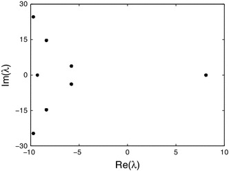
The eigenvalues of the fixed point  for
for  , and
, and  . Thus the homoclinic orbit can be classified as one of saddle-focus type with saddle-quantity
Numerical continuation of waves
Here we start with the derivation of an equivalent DDE in a co-moving frame for the travelling waves. This is a standard approach and normally would allow us to study periodic orbits that relate to waves in the original system. However, we found that for the available numerical tools to work we needed to modify the equations artificially. Therefore we computed the waves in an alternative and novel way. Rather than using a PDE approach we inserted the co-moving frame directly and used the discretisation of that system as described below.
A delay differential equation for waves
We write  and transform (4) to a delayed partial differential equation (DPDE) using Fourier techniques (see (Coombes et al. 2003) for more details) to obtain
 |
20 |
Next we insert the wave ansatz  and obtain the following delay differential equation (DDE)
 |
21 |
One can make the following observations about this equivalent DDE. First, suppose we had inserted the more common ansatz  for right-going waves. We would then have obtained an advanced instead of a delayed term. Also, this time rescaling gives a constant delay which is numerically more stable. Second, for simulations one can also compute the history integral from the DDE for
  in (21). However, the history of
  , must satisfy the constraint
 |
22 |
So, if we know the history of  we actually know
  for
for  . We use system (21) to determine periodic orbits with numerical continuation. The continuation problem automatically specifies enough history so that this does not pose a problem. Solving (21) using knut (Roose and Szalai 2007) we did not achieve convergence. This can be understood from the steady state problem of system (16). This is ill-defined as any constant may be added to
  giving a continuum of solutions as we lose the constant of integration. The integral constraint yields
  and hence maximally three steady states exist. Adding a small additional term
  to
to  in (16) and (21) with
  incorporates the integral constraint. The continuation results for both system (16) and (21) were then numerically stable and in agreement with final profiles obtained from simulations.
Direct continuation of the integral equation
As the DDE-approach only works for the modified system, we develop a novel numerical scheme to track periodic solutions of the integral equation in a co-moving frame. The novelty is that we do not introduce auxilary variables as for the DDE, but compute the (convolution) integrals directly using fast Fourier transforms (FFT). Working with the non-local model (17) directly also allows us to treat a more general class of weight distributions and not only those of exponential form (though we do not pursue this here).
Similarly as for the simulations of (4) we use an equidistant spatial grid  with
with  mesh points for the interval
  . We employ central finite differences for the temporal derivative. We have one convolution with the connectivity
  . For our periodic solutions
  , this convolution can be computed by taking the FFT of
  and
and  , multiplying element-wise and then applying the inverse FFT. It is sufficient to take the FFT of
  and not its periodic summation as the connectivity
  decays sufficiently fast so that
  . Hence the circular convolution theorem can be employed. We observe that the integral over
  can be seen as another convolution of
  with
with  with
with  the Heaviside step function. It is not strictly necessary, but we have the Fourier transforms of
  and
and  analytically and can evaluate them immediately without transforming these with a FFT. For simplicity and convergence, we use
  . Next we use the periodic boundary condition
  to eliminate one equation. Then to break the translational invariance we add the integral phase condition
  where
where  is some reference solution; here we take the previously computed point. This results in
  equations for
  unknowns. Then we use the pseudo-arclength condition
  , where
  is the tangent vector,
  is the step-size and the brackets indicate the standard inner-product (Meijer et al. 2009). We add the spatial period
  as an additional parameter.
Initial data for the continuation
The numerical continuation of travelling waves needs an initial point sufficiently close to an actual solution branch. There are two ways to obtain such data. The first is to take parameters corresponding to a Turing instability. The initial profile is then  . The second way is to use a simulation where
  approaches a travelling wave. Then the final profile
  of
of  can be used as initial point for the continuation. This is sufficient for our novel method. For the DDE, we need the auxilary variables
  along the periodic orbit. For
  we integrated
  with the trapezoidal rule over
  . Convoluting
  with the connectivity
  yields
  and
and  is obtained from numerical differentation of
  . The initial parameters are the same as in the simulation.
Parameter dependence of the travelling waves
From Fig. 2 we find Turing instabilities for  at
at  and
and  with
with  and
and  , respectively. Starting the numerical continuation from
  and varying
  we find travelling waves, see Fig. 6. First they are unstable, but the branch turns at
  where the travelling waves are stable until
  . In between, near
  , there is bistability of two different waves where the branch turns twice. The difference in the profile is an additional local minimum, present for lower values of
  . Finally, the branch ends at
  . For
. For  there is only one Turing instability for
  with
with  . Following this branch we encounter similar scenarios, but the branch ends by approaching a non-uniform stationary profile near
  when the speed
  vanishes. Also the amplitude shows that the wave emanates from these Turing points (at
  ). The amplitude of travelling waves near Turing points is also illustrated in Fig. 7. This shows for fixed
  that the prediction of the amplitude equations and results of the numerical continuation match well. We were unable to observe these small amplitude waves in simulations close to the Turing points corroborating that these bifurcations are subcritical. We have also investigated the effect of other system parameters, see Fig. 8. For decreasing
  the wave speed increases as waves more easily excite neighbouring tissue. Increasing
  leads to faster stable waves.
Fig. 6.
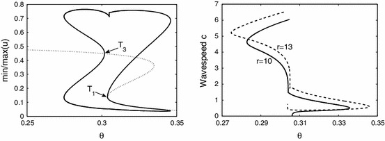
Left The minima and maxima of the wave profile for varying  for
for  (solid line). The wave emanates from the Turing points at
  from the homogeneous fixed point (dotted line). Right The dependence of the wavespeed when varying the threshold
  for
for  (solid) and
  (dashed). The waves with maximal amplitude are stable, the others are unstable. Spatial domain always fixed to
  and
and 
Fig. 7.
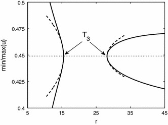
The minima and maxima of the wave profile varying  for
for  (solid line). The travelling wave emanates from Turing points at
  for
for  from the steady state (dotted line). The amplitude predicted by the weakly nonlinear analysis is indicated by dashed lines. Spatial domain always fixed to
  and
and 
Fig. 8.
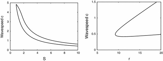
The dependence of the wavespeed for the 1 pulse solution when varying connectivity scale  (left) and refractory time
  (right). The upper (lower) branch corresponds to stable (unstable) solutions. Spatial domain always fixed to
Dispersion curves and kinematic theory
Figure 9 shows the dependence of the wave speed on the spatial period  . The direct continuation of the integral equation and those obtained using (21) agreed very well, i.e. to the first four digits.
Fig. 9.
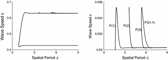
Dispersion curves of travelling waves with N=1–3 pulses. Left enlargement near the upper branch. The symbols
 indicate the number of pulses within a period
  and
and  differs from
  in that the interpulse distance is different, see Fig. 11. The
  solution is expected to be stable (using a kinematic analysis) when
A kinematic theory of wave propagation is one attempt to follow the progress of localised pulse shapes, within a periodic wave, at the expense of a detailed description of their shape (Rinzel and Maginu 1984). Suppose that a pulse has a well defined arrival time at some position  then we denote the arrival of the
  th pulse at position
  by
by  . A periodic wave, of period
  , is then completely specified by the set of ordinary differential equations
 |
23 |
with solution  , where
  is the dispersion curve, such as that obtained numerically in Fig. 9. The kinematic formalism asserts that there is a description of irregular spike trains in the above form such that
 |
24 |
where  is recognised as the instantaneous period of the wave train at position
  . A steadily propagating wave train is stable if under the perturbation
  the system converges to the unperturbed solution during propagation, or
  as
as  . For the case of uniformly propagating periodic traveling waves of period
  we insert the perturbed solution in (23), so that to first order in the
 |
25 |
Thus, a uniformly spaced, infinite wave train with period  is stable (within the kinematic approximation) if and only if
  . Hence, for the dispersion curves of shown in Fig. 9 it would seem to a first approximation that it is always the faster of the two periodic branches that is stable. Note that where there are bumps in the dispersion curve defining so-called supernormal wave speeds (wave speeds are faster than the corresponding speed of the large period wave) then it is only the supernormal wave of smaller period that is stable. Corresponding conclusions can also be made about subnormal waves (waves of slower speed compared to the wave of large period) on the slower branch. Also shown in Fig. 9 are waves with multiple pulses per period
  and we indicate the number
  of pulses on a branch by
  .
.
According to the kinematic prediction there is a change of stability at the stationary points of the dispersion curve, i.e. the extrema in Fig. 9. As the branch persists another solution branch must bifurcate from a stationary point. Therefore we expect these points to act as organising centers of the waves. Indeed with (21) we have verified that the 2-pulse solution starts from a period-doubling bifurcation very close to the highest stationary point. In addition we plotted the dispersion curve with  , i.e. period per pulse, see Fig. 10. This may be demonstrated on an infinite domain, but here we show the following simulations. Consider a periodic domain
  , where the
  dispersion curve has positive slope. If we consider two pulses at equal distance then this is equivalent to the
  branch at
  . Indeed, this is the result found in Fig. 4 (right), where we determined the wavespeed
  . Now we take a slightly displaced double one-pulse solution, i.e. one pulse starts at
  and the other at
  . Initially these pulses travel as two separate pulses but then adjust their speeds, and inter-pulse time, to travel together at a slightly lower speed
  , see Fig. 10.
Fig. 10.
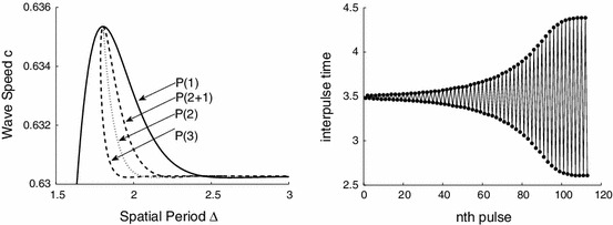
Left Scaled dispersion curves on the upper branch. Right The inter-pulse time for successive pulses for  and two pulses in the domain. Initially equal as along the P(1) dispersion curve and then as along the P(2) branch. See the animation (Online Resource 1) for the simulation
The travelling wave solution with three pulses corroborated the chaotic saddle-focus scenario even further as it formed an isolated branch in a two parameter diagram as expected, Fig. 11 (left). Interestingly we found that the  and
and  branch were different in the inter-peak distance, see Fig. 11 (right). On the
  branch the three pulses travel together where the distance between the first and second and that of the second and third is nearly equal around
  , while on the
  branch the third pulse follows at a distance of
  from the second.
Fig. 11.
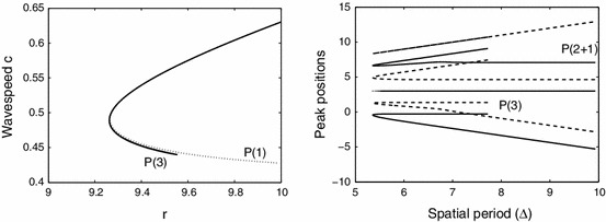
Left The 3 pulse solution forms an isolated branch in a two parameter diagram. Right The spatial positions of the peaks of the pulses on the three pulse branch. We have plotted two fundamental domains and centred the six pulses around the third pulse
Discussion
We have considered periodic travelling waves in a one dimensional neural field model describing a single spatially extended population with purely excitatory interactions. Importantly we have included an absolute refractory process as in the original work of Wilson and Cowan (1972) and shown how to analyse this using a mixture of linear (Turing) analysis and novel numerical techniques. Despite the long history and extensive study of this type of model, to the best of our knowledge this is the first analysis of moving  -pulses in a neural field model with refractoriness. Moreover, we have shown that the types of travelling pulse patterns in this class of neural field model can be captured with a reduced kinematic description. This highlights the importance of the shape of the dispersion curve and its usefulness in predicting the behaviour of more exotic travelling wave packets. Given that other variants of neural field models, such as those that include axonal delays (Venkov et al. 2007), synaptic depression (Kilpatrick and Bressloff 2010), and slow inhibitory feedback (Taylor and Baier 2011) are also known to support periodic travelling waves it is of interest to construct dispersion curves for these models and contrast their shapes (and in effect the types of wave that they would be able to support). This is a topic of ongoing research and will be reported upon elsewhere.
Electronic supplementary material
Below is the link to the electronic supplementary material.
Acknowledgments
Open Access
This article is distributed under the terms of the Creative Commons Attribution License which permits any use, distribution, and reproduction in any medium, provided the original author(s) and the source are credited.
Appendix
Let us consider the value of  at the bifurcation point to be given by
  with corresponding values of
  and
and  as
as  and
and  respectively. We consider an asymptotic expansion for
  in the form
  , where
  . After setting
  and
and  we then substitute into (4), making use of the fact that
  and
and  . Equating powers of
  leads to a hierarchy of equations:
 |
26 |
 |
27 |
 |
28 |
 |
29 |
where
 |
30 |
and
 |
31 |
Here  and
and  . The first equation (26) fixes the steady state
  . The second equation (27) is linear with solutions
  , which is equivalent to saying that the kernel of
  is spanned by the functions
  . A dynamical equation for the complex amplitudes
  (and we do not treat here any slow spatial variation) can be obtained by deriving solvability conditions for the higher-order equations, a method known as the Fredholm alternative. These equations have the general form
  (with
(with  ). We define the inner product of two periodic functions (with spatial periodicity
  and temporal periodicity
  ) as
) as
 |
32 |
where  denotes complex conjugation. The adjoint of
  with respect to this inner product can be found as
 |
33 |
where
 |
34 |
We observe that the kernel of  is spanned by the same set of functions as the kernel of
  . Hence the solvability condition takes the form
 |
35 |
The solvability condition with  is automatically satisfied. A comparison of the terms in (28) suggests writing
  in the form
 |
36 |
For  the calculation of the solvability condition, projecting onto
  , is facilitated with the following results
 |
37 |
Here  (after using the bifurcation condition
  ). Substitution of (36) into (28) and equating powers of exponentials gives
  and
and  where
where
 |
38 |
 |
39 |
 |
40 |
 |
41 |
Finally using  and the above results gives Eq. (14) with
 |
42 |
 |
43 |
 |
44 |
A similar analysis, projecting onto  , yields (15).
References
- Beurle RL (1956) Properties of a mass of cells capable of regenerating pulses. Philos Trans R Soc Lond B 240:55–94
- Bressloff PC. Spatiotemporal dynamics of continuum neural fields. J Phys A. 2012;45:033001. doi: 10.1088/1751-8113/45/3/033001. [DOI] [Google Scholar]
- Coombes S, et al. Neural field theory, chap. Tutorial on neural field theory. Verlag: Springer; 2013. [Google Scholar]
- Coombes S, et al. Waves and bumps in neuronal networks with axo-dendritic synaptic interactions. Phys D. 2003;178:219–241. doi: 10.1016/S0167-2789(03)00002-2. [DOI] [Google Scholar]
- Curtu R, Ermentrout B. Oscillations in a refractory neural net. J Math Biol. 2001;43:81–100. doi: 10.1007/s002850100089. [DOI] [PubMed] [Google Scholar]
- Curtu R, Ermentrout B. Pattern formation in a network of excitatory and inhibitory cells with adaptation. SIAM J Appl Dyn Syst. 2004;3:191–231. doi: 10.1137/030600503. [DOI] [Google Scholar]
- Ermentrout GB. Neural nets as spatio-temporal pattern forming systems. Rep Prog Phys. 1998;61:353–430. doi: 10.1088/0034-4885/61/4/002. [DOI] [Google Scholar]
- Ermentrout GB, McLeod JB. Existence and uniqueness of travelling waves for a neural network. Proc R Soc Edinb A. 1993;123:461–478. doi: 10.1017/S030821050002583X. [DOI] [Google Scholar]
- Evans JW, et al. Double impulse solutions in nerve axon equations. SIAM J Appl Math. 1982;42:219–234. doi: 10.1137/0142016. [DOI] [Google Scholar]
- Feroe JA. Existence and stability of multiple impulse solutions of a nerve equation. SIAM J Appl Math. 1982;42:235–246. doi: 10.1137/0142017. [DOI] [Google Scholar]
- Gonchenko SV, et al. Complexity in the bifurcation structure of homoclinic loops to a saddle-focus. Nonlinearity. 1997;10(2):409–423. doi: 10.1088/0951-7715/10/2/006. [DOI] [Google Scholar]
- Hastings SP. Single and multiple pulse waves for the FitzHugh-Nagumo equations. SIAM J Appl Math. 1982;42:247–260. doi: 10.1137/0142018. [DOI] [Google Scholar]
- Hoyle R. Pattern formation: an introduction to methods. London: Cambridge University Press; 2006. [Google Scholar]
- Huang X, et al. Spiral waves in disinhibited mammalian neocortex. J Neurosci. 2004;24:9897–9902. doi: 10.1523/JNEUROSCI.2705-04.2004. [DOI] [PMC free article] [PubMed] [Google Scholar]
- Keener J, Sneyd J. Mathematical physiology. Verlag: Springer; 1998. [Google Scholar]
- Kilpatrick ZP, Bressloff PC. Spatially structured oscillations in a two-dimensional neuronal network with synaptic depression. J Comput Neurosci. 2010;28:193–209. doi: 10.1007/s10827-009-0199-6. [DOI] [PubMed] [Google Scholar]
- Kuznetsov YA. Impulses of a complicated form in models of nerve conduction. Selecta Mathematica (formerly Sovietica) 1994;13:127–142. [Google Scholar]
- Lin XB. Using Melnikov’s method to solve Silnikov’s problems. Proc R Soc Edinb A. 1990;116:295–325. doi: 10.1017/S0308210500031528. [DOI] [Google Scholar]
- Lord GJ, Coombes S. Traveling waves in the Baer and Rinzel model of spine studded dendritic tissue. Phys D. 2002;161:1–20. doi: 10.1016/S0167-2789(01)00339-6. [DOI] [Google Scholar]
- Meijer HGE, et al. Numerical bifurcation analysis. In: Meyers RA, et al., editors. Encyclopedia of complexity and systems science. New York: Springer; 2009. pp. 6329–6352. [Google Scholar]
- Miller RN, Rinzel J. The dependence of impulse propagation speed on firing frequency, dispersion, for the Hodgkin-Huxley model. Biophys J. 1981;34:227–259. doi: 10.1016/S0006-3495(81)84847-3. [DOI] [PMC free article] [PubMed] [Google Scholar]
- Pinto DJ, Ermentrout GB (2001) Spatially structured activity in synaptically coupled neuronal networks: I. Travelling fronts and pulses. SIAM J Appl Math 62:206–225
- Rinzel J, Maginu K. Kinematic analysis of wave pattern formation in excitable media. In: Vidal C, Pacault A, editors. Non-equilibrium dynamics in chemical systems. Verlag: Springer; 1984. pp. 107–113. [Google Scholar]
- Röder G, et al. Wave trains in an excitable FitzHugh-Nagumo model: bistable dispersion relation and formation of isolas. Phys Rev E. 2007;75:036202. doi: 10.1103/PhysRevE.75.036202. [DOI] [PubMed] [Google Scholar]
- Roose D, Szalai R (2007) Continuation methods for dynamical systems: path following and boundary value problems. Continuation and bifurcation analysis of delay differential equations, Springer-Canopus, Verlag, pp 359–399
- Taylor PN, Baier G. A spatially extended model for macroscopic spike-wave discharges. J Comput Neurosci. 2011;31:679–684. doi: 10.1007/s10827-011-0332-1. [DOI] [PubMed] [Google Scholar]
- Venkov NA, et al. Dynamic instabilities in scalar neural field equations with space-dependent delays. Phys D. 2007;232:1–15. doi: 10.1016/j.physd.2007.04.011. [DOI] [Google Scholar]
- Wilson HR, Cowan JD. Excitatory and inhibitory interactions in localized populations of model neurons. Biophys J. 1972;12:1–24. doi: 10.1016/S0006-3495(72)86068-5. [DOI] [PMC free article] [PubMed] [Google Scholar]
- Wilson HR, Cowan JD (1973) A mathematical theory of the functional dynamics of cortical and thalamic nervous tissue. Kybernetik 13:55–80 [DOI] [PubMed]
Associated Data
This section collects any data citations, data availability statements, or supplementary materials included in this article.