Level Set Segmentation of Breast Masses in Contrast-Enhanced Dedicated Breast CT and Evaluation of Stopping Criteria

Abstract

Dedicated breast CT (bCT) produces high-resolution 3D tomographic images of the breast, fully resolving fibroglandular tissue structures within the breast and allowing for breast lesion detection and assessment in 3D. In order to enable quantitative analysis, such as volumetrics, automated lesion segmentation on bCT is highly desirable. In addition, accurate output from CAD (computer-aided detection/diagnosis) methods depends on sufficient segmentation of lesions. Thus, in this study, we present a 3D lesion segmentation method for breast masses in contrast-enhanced bCT images. The segmentation algorithm follows a two-step approach. First, 3D radial-gradient index segmentation is used to obtain a crude initial contour, which is then refined by a 3D level set-based active contour algorithm. The data set included contrast-enhanced bCT images from 33 patients containing 38 masses (25 malignant, 13 benign). The mass centers served as input to the algorithm. In this study, three criteria for stopping the contour evolution were compared, based on (1) the change of region volume, (2) the average intensity in the segmented region increase at each iteration, and (3) the rate of change of the average intensity inside and outside the segmented region. Lesion segmentation was evaluated by computing the overlap ratio between computer segmentations and manually drawn lesion outlines. For each lesion, the overlap ratio was averaged across coronal, sagittal, and axial planes. The average overlap ratios for the three stopping criteria ranged from 0.66 to 0.68 (dice coefficient of 0.80 to 0.81), indicating that the proposed segmentation procedure is promising for use in quantitative dedicated bCT analyses.

Introduction

Over the past three decades, mammography has been the most widely used screening tool for breast cancer. Although the mortality rate has been shown to be significantly reduced by 30 to 40 % in screened populations [1], the poor positive predictive value (4 to 9 % for mammography screening, 39.5 % for biopsy performed based on diagnostic mammography) [2] indicates potential for improvement. The high rate of misdiagnosis is in part due to tissue superimposition, which occurs when complex 3D tissue structures are projected onto a plane [1]. The resulting anatomic noise makes lesion visualization difficult, potentially causing a false negative, or it can mimic the appearance of a cancer, potentially causing a false positive. As a result, misdiagnosis on mammography ultimately increases healthcare costs, as well as unnecessary patient anxiety and biopsies.

Recently, researchers have been developing dedicated breast CT (bCT) systems, which produce 3D images of the breast and mitigate superimposition effects in mammography [1, 3–5]. This emerging technology not only produces excellent morphologic details but also provides higher tumor contrast. Initial clinical reports revealed that breast CT has better conspicuity in mass visualization over mammography and concluded that bCT is promising and is likely to play a significant role in future breast cancer screening and diagnosis [6, 7]. However, bCT substantially increases the amount of data that radiologists need to review. In our dataset, a typical image volume of one breast includes 512 slices for transverse and sagittal planes and over 300 slices for coronal planes. Thus, to provide a decision support to the radiologists, we are developing a CAD scheme for dedicated bCT, which requires accurate segmentation of the lesion from surrounding tissues.

In an initial study, masses in bCT images were segmented using the radial gradient index (RGI) algorithm [8, 9]. For 93 % of the masses, the automated segmentation yielded an overlap ratio of 0.4 or greater. However, lesion segmentations tended to be undergrown and too spherical. Ray et al. developed a semi-automated segmentation for masses in dedicated bCT based on the watershed algorithm [10, 11]. Their method requires the user to input several markers to initialize the segmentation. The algorithm presented here requires only the lesion center as input, which is provided by a radiologist but could alternatively result from the output of a lesion detection (CADe) algorithm. Other than our initial study [8], to the best of our knowledge, this is the first algorithm for automated seeded lesion segmentation on bCT.

Active contour (or “snake”) segmentation was originally proposed by Kass et al. [12]. This model seeks an object margin that minimizes an energy functional consisting of internal energy and external energy along the deformable contour. Active contour segmentation has been used in medical imaging [13–16]. In breast imaging, Brake et al. used a discrete active contour method to segment mammographic mass lesions [17]. Sahiner et al. incorporated edge and region analysis to help minimize the contour energy [18]. Both works express the contour as an N-points polygon, making the handling of topology changes difficult, as seen in split and merge segmentation methods. To solve this problem, Yuan et al. [19] proposed a level set-based approach [20–22] that can handle splitting and merging in a natural way for segmenting masses on mammogram. In this work, we extend this level set approach to 3D, and use the previously developed RGI segmentation to generate the initial contour.

Contour leaking is a problem in lesion segmentation on medical images due to the presence of ambiguous margins. Therefore, a stopping criterion is required to terminate the iterative contour evolution process at the lesion margin. In this study, we developed and compared three stopping criteria based on (1) the change of segmented region volume at each iteration, (2) the average intensity in the segmented region increase at every iteration, and (3) the rate of change of the average intensity inside and outside the segmented region [19].

This paper is organized as follows: Section “Materials and Methods” introduces the database for this study and the proposed segmentation procedure. Section “Results” displays the results. Section “Discussion” and “Conclusion” give a discussion and conclusion, respectively.

Materials and Methods

Image Dataset

The dataset included 33 contrast-enhanced breast CT images, containing 38 masses [25 malignant masses, 13 benign masses] acquired at the University of California at Davis under an IRB-approved protocol. The voxel dimensions in the coronal plane were equal and varied between 200 and 400 μm, and were different from coronal slice spacing. Lesions were manually outlined in the coronal, sagittal, and axial planes by a research specialist with over 15 years of experience in mammography research.

Segmentation Algorithm

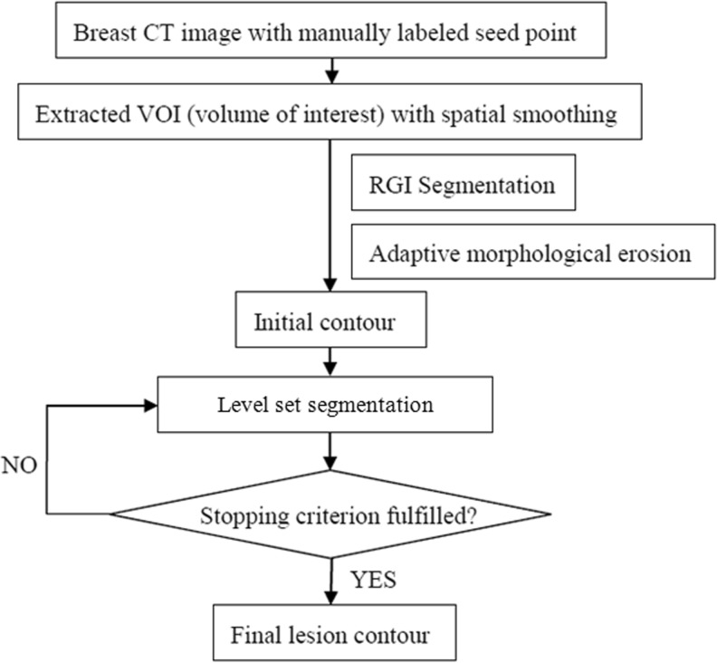
Figure 1 shows the flow chart of the proposed segmentation algorithm. Our segmentation is performed in two stages: contour initialization with the RGI algorithm followed by a level set-based active contour model.

Fig. 1.

Schematic of the seeded breast CT lesion segmentation algorithm

Although the level set-based active contour algorithm can handle topologic changes in a natural way and is expected to be able to capture complicated morphologic details, the way it minimizes the energy functional is complex and can result in errors on noisy and ambiguous images, such as medical images. Since breast lesions tend to exhibit local intensity variations, and lesions occur in a wide variety of sizes and shapes, it is not guaranteed that the active contour evolution equation always finds the global minimum that represents the optimized image partition. As a result, the evolving contour might become trapped in a local minimum of the energy functional. One way to guide contour evolution towards the global minimum is to initialize the active contour segmentation with an approximated lesion contour that is sufficiently enough to the true lesion margin to avoid local minima.

Based on our previous study [8], RGI can produce an approximate contour in a very short amount of time, with the limitation of the contours being too spherical and sometimes undergrown. While these limitations can produce unsatisfactory lesion outlines, they make the RGI algorithm well-suited for contour initialization, which requires the contour to be entirely contained within the lesion. Thus, in the proposed segmentation algorithm, we use RGI segmentation to generate the initial approximate lesion outline, and use an active contour model to evolve the lesion contour towards the desired location and to capture morphologic details for greater segmentation accuracy.

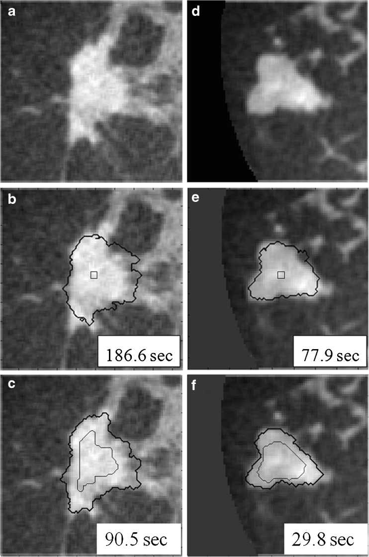
Figure 2 shows the difference in segmentation results with and without use of a RGI-approximated initial lesion contour. As shown in Fig. 2, RGI segmentation not only increases the efficiency of the overall segmentation procedure, it also helps improve the accuracy for the second stage of segmentation.

Fig. 2.

Comparison of active contour segmentation with different initial contours. a, d Coronal views of two dedicated breast CT lesions; b, e The initial contour was a cubic surface of 3³ voxels; c, f The initial contour was, as included in our proposed overall segmentation method, an eroded RGI segmentation. Thin lines: initial contour; thick lines: final segmentation

Contour Initialization

RGI segmentation is a seeded lesion segmentation technique [9]. Reiser et al. extended it into 3D and showed that it can be applied on dedicated breast CT images [8]. For a given lesion contour dΩ, the 3D RGI is given by:

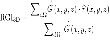1

where is the image gradient, and is a unit vector in the radial direction.

The volume of interest is multiplied by a 3D Gaussian constraint function, then a series of contours dΩ_i are generated by applying multiple gray-level thresholds to the constrained VOI. The resulting segmentation is the contour that maximizes RGI:

2

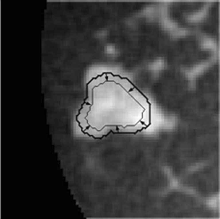
In this algorithm, the standard deviation of the Gaussian constraint function was 10 mm, based on Reiser et al.’s study [8]. Further, to ensure that the initial contour is completely contained within the lesion before the second segmentation stage, morphological erosion is applied to shrink the RGI segmented lesion contour by using the MATLAB function “imerode” with a cubic structuring element. The side length of the structuring element was one ninth of the cube root of the RGI segmented lesion volume. The resulting contour then served as the initial contour for the subsequent active contour segmentation. Figure 3 shows an example of a mass with a RGI segmented contour and the eroded contour, which is used to initialize the level set segmentation. Details about the active contour model are described in the following sections.

Fig. 3.

Demonstration of the RGI segmented contour (bold contour line) and the subsequently-eroded contour (thin contour line), which serves as the initial contour for input to the active contour segmentation stage

Original Level Set Model

The level set-based propagating fronts theory for delineating shapes on an image was introduced in 1988 [20]. The central idea of a level set method is to express the contour as the zero level set of a higher-dimensional function, the so-called level set function. The evolving contour is formulated through the evolution of the level set function; i.e. dΩ is the zero level set: dΩ = {(x, y, z) | φ(x, t) = 0}, φ(x, t) is the evolving level set function and t is the iteration. Let x be a location vector ∊  on the evolving hypersurface and F(x) a speed function normal to the front at x, and thus, the evolution equation for φ can be given as a basic formulation of a “Hamilton–Jacobi type” equation [20–22]:

3

In this classical level set front propagating equation, the level set function φ, however, can develop shocks, i.e., very sharp or flat shapes during evolution. Among different approaches to resolve this problem, Li et al. proposed a regularization term given as [23] :

4

where R(φ) is the regularization functional. The basic idea of this regularization term is to maintain the evolving level set function as a signed distance function with its intrinsic property |∇φ| = 1. This regularization term avoids contour re-initialization, which is computationally expensive [24, 25].

Combining the Hamilton–Jacobi type equation (Eq. 3) and the regularizing term (Eq. 4) yields the level set evolution equation:

5

where F is the speed function normal to x; ν is a scalar parameter that controls the direction of front propagation (negative value if evolving outward and positive if evolving inward); τ is the iteration step size; k is the iteration number; and g is the indicator function, given by:

6

where G_σ is a Gaussian kernel and I is the image array. The indicator function was introduced by Castelles et al. and is often seen in level set-based curve evolution in image processing and computer vision applications [21]. It incorporates geometrical information into the level-set function and ensures that the contour stops evolving in edge-like regions [21].

Since |∇φ| = 1 is enforced by the regularizing term (i.e., the term in square brackets on the right hand side of Eq. (5)), the last, so-called fronts propagating term can be simplified as νgF. In addition, by letting F be a delta function, the propagating front uniformly expands:

7

where ɛ controls the sharpness of the delta function. Its value, ɛ = 0.2, was based on Li et al.’s settings [23].

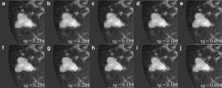
For large lesions in our dataset, active contour segmentation could be very time consuming and therefore, the selection of τ had to be larger than 1,000 to complete the segmentation task to reduce computation time for cases with large masses. For the purpose of stability, Li et al. suggested that the product of τ and μ should be less than 0.25 [23]. To reach this, a small value of μ is often chosen which in turn somewhat suppresses the effect of the regularization term. In this study, we found that the need of a large value of τ could yield undesired segmentation results even if τμ is less than 0.25 (Fig. 4a–e). This is because the strength of the regularization term, which is multiplied by τ, is comparatively larger than the fronts propagating term when it is significantly suppressed by g around the lesion margin. As a result, the regularization term can produce noise during contour evolution, cause erroneous termination, and might enable the contour to cross over the barrier set up by g, ultimately producing unsatisfying segmentation results. Figure 4a–e shows segmentations obtained with τ = 1,000 and different values of μ.

Fig. 4.

a–e Dedicated breast CT lesion segmentations obtained for different values of τμ using Eq. 5. f–j Dedicated breast CT lesion segmentations obtained for different values of τμ using Eq. 9. The coronal plane is shown. The stopping criterion was

Proposed Modified Level Set Algorithm

Since the purpose of the regularization term is to maintain the signed distance function property only during the evolution process, the regularizing function becomes redundant when the evolving contour approaches the lesion margin where . To solve this problem, we propose to make the regularization term dynamic along with the contour evolution by incorporating the geometrical information into the regularization term using a “softened” indicator function g_s:

8

Hence, the level set evolution equation becomes

9

Note that compared to Eq. (6), the power of |∇G_σ * I| in the denominator of g_s is 1 rather than 2. From our experiments, we noticed that if g is used instead of g_s, the level set function can still produce subtle instability around the lesion margin because the regularization term is suppressed slightly too early. Figure 4f–j shows segmentation results from the new model that incorporates g_s, with τ = 1,000 and different values of μ and for the same case as shown in Fig. 4a–e. Here we suggest τμ < 0.15 for 3D bCT images, because τμ > 0.15 can still cause instabilities as shown in Fig. 4f, g.

Figure 5 shows a comparison of the segmentation results from the model without and with the softened indicator function (Fig. 5b, d) and the corresponding human-delineated outline (Fig. 5a). In Fig. 5d the evolution stops automatically due to the stopping criterion, while the evolving contour shown in Fig. 5b has already crossed over the lesion margin at 60 iterations yielding poor segmentation performance. Figure 5c, e shows the corresponding regularization term maps.

Fig. 5.

a Human-delineated lesion outline of the bCT lesion. b Segmentation result using Eq. 5. c Corresponding regularization map. d Segmentation result using Eq. 9. e Corresponding regularization map. Examples are displayed in the coronal plane. VOI size was 36 × 36 × 35.5 mm

Stopping Criteria

In our preliminary study, we developed and compared three stopping criteria [26]:

1. The first stopping criterion is the minimum of ΔV/V, and is based on the change of segmented region volume. Given the segmented volume V and the difference in region volume from the previous to the current iteration step ΔV, contour evolution is terminated when ΔV/V reaches a global minimum.

2. The second stopping criterion is the minimum of , and is based on the average voxel intensity within the segmented region increase at each iteration. Here, Ω denotes the segmented region and ΔΩ = Ω_t+1 − Ω_t is its increase in two consecutive iteration steps, and is the average voxel intensity in ΔΩ. When the contour approaches the lesion margin, is expected to decrease significantly. Therefore we select the 3D contour that corresponds to the global minimum of the derivative as the final lesion margin.

3. The third stopping criterion, , is based on comparing the rate of change (i.e., the slope) of the average voxel intensity as a function of iteration number inside and outside the segmented region, and was initially proposed by Yuan et al. [19]. Denoting the average voxel intensities inside the segmented region as , outside the segmentation as , and along the contour as , the difference of rates of change of average intensities inside and outside the segmented region are given as

   10

   where V_B is the volume of the VOI excluding the segmented lesion. Note that parameters of this equation were adjusted for 3D bCT images. When the evolving contour crosses the lesion margin, the rate of change of the average intensity inside the segmented region increases, and will eventually match that outside the segmentation. Therefore the contour evolution is terminated when the rate difference, , reaches zero. Since a numerical comparison against zero is difficult, for practical purposes, contour evolution was terminated when was less than 0.5.

Evaluation

Manual lesion outlines on three orthogonal planes, drawn by a research specialist in mammography, served as a reference for evaluating the segmentation algorithm. Segmentation performance was assessed as the average overlap ratio (OR_avg ), computed as:

11

where Ω_2D is a cut through the 3D computer-segmentation that includes the lesion center, and (cor), (sag), and (ax) denote the orientation of the plane. ω_man is the human-delineated lesion outline in the same plane [8]. The computer outlines produced by the three stopping criteria were compared in terms of OR_avg, averaged over all cases. A t test [27] was used to compare the performances across the three stopping criteria.

Results

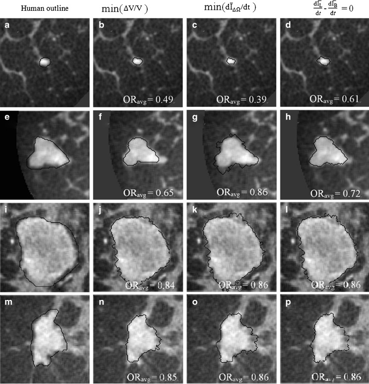
Figure 6 shows examples of segmentation results by using the proposed active contour model with the three stopping criteria, for four masses. The leftmost column shows the manual outline of each mass. This figure also illustrates the variability of size, shape, and intensity variations within and in the neighborhood of breast masses imaged with 3D bCT.

Fig. 6.

Segmentation examples for the three stopping criteria. τμ = 0.10

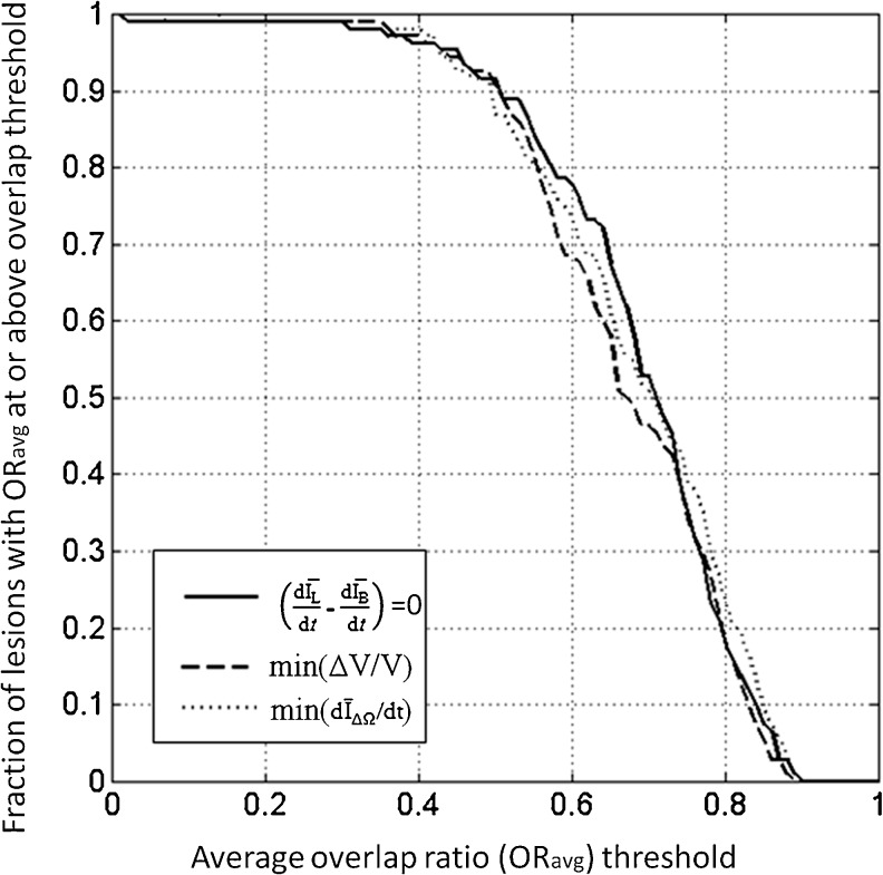
Figure 7 plots the proportion of correctly segmented masses, as a function of OR_avg threshold. For all three stopping criteria, OR_avg was greater than 0.4 for 96 % of all masses. Overall, all stopping criteria produced similar curves, but for much of the range of OR_avg thresholds, the min(ΔV/V) criterion resulted in a smaller proportion of correctly segmented masses, compared to the other two stopping criteria. Note that an overlap ratio of 0.4 corresponds approximately to a DICE coefficient of 0.57.

Fig. 7.

Segmentation performance as a function of OR_ave threshold, for the three stopping criteria

Table 1 presents the performance of the proposed automated segmentation scheme for the three stopping criteria in terms of <OR_avg>, where <•> indicates average across all cases. For all stopping criteria, <OR_avg> was 0.66 or greater, corresponding to a DICE coefficient of about 0.79 (Appendix A). A DICE coefficient of at least 0.7 was found to be appropriate for computer segmentation [28].

Table 1.

Segmentation performance in terms of averaged overlap ratio for the three stopping criteria and comparison results in terms of p values from the t test

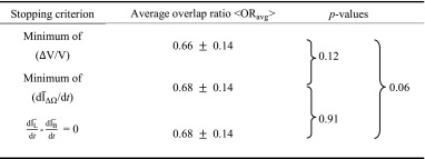
The similarity of the lesion segmentations was assessed using a pairwise t test. No statistically significant differences were found.

Discussion

Figures 4 and 5 demonstrate the effect of multiplying the regularization term with a “softened” indicator function (Eq. 9), which not only ensures that |∇φ| = 1 during contour evolution, but also prevents the regularization map from developing undesired results when the driving force is being suppressed and the evolving contour approaches the stopping point (Fig. 5).

Overall, the proposed segmentation algorithm produces satisfactory lesion outlines for all stopping criteria in the sense that surrounding glandular tissues are not included in the segmented region (Fig. 6i–l). As shown in Fig. 6, the active contour model evolves contours smoothly without generating shocks. The regularization term plays an important role in maintaining the stability. When |∇φ| > 1, the regularization term [∇²φ − div (∇φ/|∇φ|)] becomes positive and tends to allow for faster expansion of the evolving contour. If |∇φ| < 1, then [∇²φ − div (∇φ/|∇φ|)] becomes negative and the contour evolves more slowly, bringing φ back toward |∇φ| = 1. This mechanism ensures that the level set function maintains its intrinsic property of a signed distance function during the evolution, |∇φ| = 1, mitigating the need for re-initialization.

Of the three stopping criteria that were investigated, min was found to be the least consistent. For small lesions, the average intensity within the grown region, , is reduced substantially during early iterations due to the small size of the segmented region. This can cause contour evolution to be terminated prematurely, as shown in Fig. 6c. For larger lesions, on the other hand, the min stopping criterion tended to be satisfied at a higher iteration number, compared to the other stopping criteria, producing slightly larger lesion segmentations. In turn, these resulted in a higher overlap ratio because the manual outlines were also drawn loosely, overestimating the lesion margin (see Fig. 6g, e). Thus, segmentations resulting in a higher overlap ratio were not necessarily closer to the lesion margin, judging by visual inspection. Furthermore, the “redundantly” grown parts (see protuberances in Fig. 6g) occurred because a large portion of background needed to be included in ΔΩ to produce a global minimum in .

Although contours from stopping criteria based on min(∆V/V) and generated similar overlap ratios, min(∆V/V) tended to produce tighter lesion outlines than the other two criteria. This can be seen in Table 1, in which min(∆V/V) produces the smallest average overlap ratio. Also, the p values of comparisons between OR_avg from segmentations with the min(∆V/V) criterion and that using the other two stopping criteria might indicate such a trend as well.

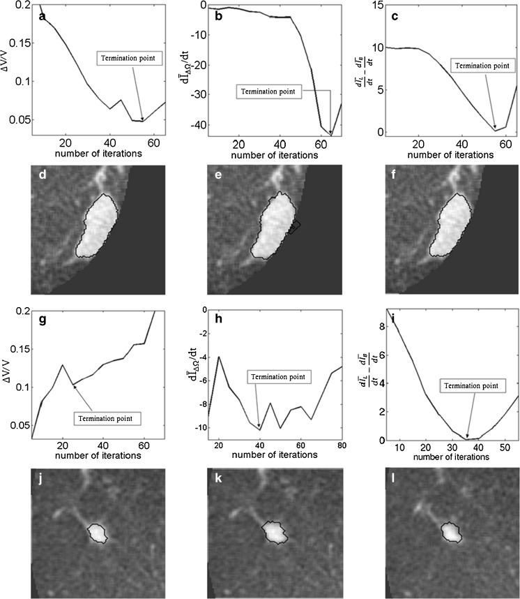
A drawback of the stopping criteria min(∆V/V) and min is the need to let the contour evolve for many iterations past the actual stopping point in order to identify the minimum, as demonstrated in Fig. 8a, g, h. If the curve is noisy, curve fitting can help to determine a reliable minimum. As shown in Fig. 8a, the segmentation will automatically cease at a local minimum if no curve fitting is used, similar to what is seen for the stopping criterion min . Due to curve fluctuations, the global minima of ∆ V/V and were selected after monitoring the contour evolution for many iterations beyond the actual stopping point (Fig. 8). In contrast, compares the average intensity inside the entire segmented region and the background and is therefore less sensitive to the intensity variations that might occur in a certain local region. As a result, is a monotonically decreasing curve that allows for easier identification of the stopping point (Fig. 8c, i).

Fig. 8.

Stopping conditions as a function of iteration number, illustrated for two different masses (top two rows, bottom two rows). a, g—ΔV/V; b, h ; and c, i . The segmentations corresponding to the termination point are shown in (d, j), (e, j), and (f, l), respectively

In a previous clinical report, Prionas et al. found that lesion conspicuity was greater in contrast-enhanced bCT images than in unenhanced images due to higher HU for both malignant and benign lesions [7]. In a subset of our cases for which non-contrast bCT images were available, we found that the average lesion enhancement due to the contrast agent was 31.4 HU. Therefore, the lesion margin is expected to be better visualized in contrast-enhanced bCT images, and easier for the segmentation algorithm to capture. Hence we used contrast-enhanced dedicated bCT images to develop the segmentation algorithm. In the future, the segmentation algorithm will be investigated on unenhanced bCT images, for which our preliminary results have shown promise [29].

Limitations of this study are that the data set is small (33 patients; 38 contrast-enhanced masses). This might have affected the observed p values when comparing OR_ave from the three stopping criteria. In a larger data set, one might expect to see smaller p values for the comparisons of min(Δ V/V) – and min(Δ V/V) – min in a larger data set, since the results in Table 1 indicate such a trend.

Further, manual outlines from one expert served as “ground truth” for the evaluation of the computer segmentation. Automated lesion segmentation is a central step in most CAD and quantitative analysis schemes and therefore, the segmentation performance ultimately needs to be evaluated in that context. However, as an intermediate step, lesion segmentation is often evaluated by comparing computer segmentations to human outlines, particularly in mammography [30, 31]. Sahiner et al. compared classification of breast masses in mammography based on outlines by radiologists, and computer segmentations [33]. They found similar performance for an average overlap ratio of 0.62, which supports the use of overlap ratio to assess computer segmentations.

Conclusion

In this paper, we present a two-stage 3D lesion segmentation method combining RGI segmentation with an active contour model. The RGI segmentation generates an approximate contour, which serves as initial contour for the subsequent contour evolution. The automated lesion segmentation algorithm was evaluated by computing the overlap ratio with manually drawn lesion outlines. Three stopping criteria were evaluated, which all yielded overlap ratios greater than 0.65 (corresponding to a DICE coefficient of 0.7). This suggests that the segmentation algorithm proposed in this paper can be successfully applied to masses imaged with dedicated breast CT. Among the stopping criteria that were investigated, min was found to be the least consistent and the use of either min(∆V/V) or is suggested, where the latter holds the advantage of not requiring curve fitting to identify the stopping point.

Appendix A

Other than overlap ratio index, some researchers use the dice coefficient (DICE) to evaluate the computer segmentation performance, defined as [32]

A1

where Ω is the computer-segmentation and ω_man is the human-delineated lesion outline. In terms of DICE, Zijdenbos et al. suggested that a good overlap occurs when DICE > 0.7 in their literature of image validation [28]. Kuo et al. showed the relationship between OR and DICE in their work of automated 3D breast ultrasound segmentation that an OR of 0.66 is equivalent to a DICE of 0.79 [33], which is still well above 0.7.

References

- 1.Lindfors KK, Boone JM, Newell MS, D’Orsi CJ. Dedicated breast computed tomography: the optimal cross-sectional imaging solution? Radiol Clin N Am. 2010;48:1043–1054. doi: 10.1016/j.rcl.2010.06.001. [DOI] [PMC free article] [PubMed] [Google Scholar]
- 2.D’Orsi CJ, Sickles EA. To seek perfection or not? That is the question. Radiology. 2012;265:9–11. doi: 10.1148/radiol.12121515. [DOI] [PubMed] [Google Scholar]
- 3.Glick SJ. Breast CT. Annu Rev Biomed Eng. 2007;9:501–526. doi: 10.1146/annurev.bioeng.9.060906.151924. [DOI] [PubMed] [Google Scholar]
- 4.Kalender WA, Beister M, Bioone MJ, Kolditz D, Vollmar VS, Weigel CCM. High-resolution spiral CT of the breast at very low dose: concept and feasibility considerations. Eur Radiol. 2012;22:1–8. doi: 10.1007/s00330-011-2169-4. [DOI] [PubMed] [Google Scholar]
- 5.O’Connell A, Conover DL, Zhang Y, Seifert P, Logan-Young W, Lin CFL, Sahler L, Ning R. Cone-beam CT for breast imaging: radiation dose, breast coverage, and image quality. AJR. 2010;195:496–509. doi: 10.2214/AJR.08.1017. [DOI] [PubMed] [Google Scholar]
- 6.Lindfors KK, Boone JM, Nelson TR, Yang K, Kwan ALC, Miller DF. Dedicated breast CT: initial clinical experience. Radiology. 2008;246:725–733. doi: 10.1148/radiol.2463070410. [DOI] [PMC free article] [PubMed] [Google Scholar]
- 7.Prionas ND, Lindfors KK, Ray S, Huang S, Beckett LA, Monsky WL, Boone JM. Contrast-enhanced dedicated breast CT: initial clinical experience. Radiology. 2010;256:714–723. doi: 10.1148/radiol.10092311. [DOI] [PMC free article] [PubMed] [Google Scholar]
- 8.Reiser I, Joseph SP, Nishikawa RM, Giger ML, Boone JM, Lindfors KK, Edwards A, Packard N, Moore RH, Kopans DB. Evaluation of a 3D lesion segmentation algorithm on DBT and breast CT images. Proc SPIE. 2010;7624:76242N. doi: 10.1117/12.844484. [DOI] [Google Scholar]
- 9.Kupinsiki M, Giger ML. Automated seeded lesioni segmentation on digital mammograms. IEEE Trans Med Imaging. 1998;17:510–517. doi: 10.1109/42.730396. [DOI] [PubMed] [Google Scholar]
- 10.Ray S, Prionas ND, Lindfors KK, Boone JM. Analysis of breast CT lesions using computer-aided diagnosis: an application of neural networks on extracted morphologic and texture feature. Proc SPIE. 2012;8315:83152E–1. doi: 10.1117/12.910982. [DOI] [Google Scholar]
- 11.Mancas M, Gosselin B: Fuzzy tumor segmentation based on iterative watersheds. ProcRISC, 2003 (Veldhoven, Netherland)
- 12.Kass M, Witkin A, Terzopoulos D. Snakes: active contour models. Int J Comput Vis. 1988;1:321–331. doi: 10.1007/BF00133570. [DOI] [Google Scholar]
- 13.Atkins MS, Mackiewich B. Fully automatic segmentation of the brain in MRI. IEEE Trans Med Imaging. 1998;17:98–107. doi: 10.1109/42.668699. [DOI] [PubMed] [Google Scholar]
- 14.Cootes T, Hill A, Taylor C, Haslam J. The use of active shape models for locating structures in medical images. Image Vis Comput. 1994;12:355–366. doi: 10.1016/0262-8856(94)90060-4. [DOI] [Google Scholar]
- 15.Yang J, Staib LH, Duncan JS. Neighbor-constrained segmentation with level set based 3D deformable models. IEEE Trans Med Imaging. 2004;23:940–948. doi: 10.1109/TMI.2004.830802. [DOI] [PMC free article] [PubMed] [Google Scholar]
- 16.Liu F, Zhao B, Kijewski PK. Liver segmentation for CT images using GVF snake. Med Phys. 2005;32:3699–3706. doi: 10.1118/1.2132573. [DOI] [PubMed] [Google Scholar]
- 17.Brake GM, Karssemeijer PK. Segemtation of suspicious densities in digital mammograms. Med Phys. 2001;28:259–266. doi: 10.1118/1.1339884. [DOI] [PubMed] [Google Scholar]
- 18.Sahiner B, Petrick N, Chan H, Hadjiiski LM, Paramagul C, Helvie MA, Curcan MN. Computer-aided characterization of mammographic masses: accuracy of mass segmentation and its effects on characterization. IEEE Trans Med Imaging. 2001;20:1275–1284. doi: 10.1109/42.974922. [DOI] [PubMed] [Google Scholar]
- 19.Yuan Y, Giger ML, Li H, Suzuki K, Sennett C. A dual-stage method for lesion segmentation on digital mammograms. Med Phys. 2007;34:4180–4193. doi: 10.1118/1.2790837. [DOI] [PubMed] [Google Scholar]
- 20.Osher S, Sethian JA. Fronts propagating with curvature-dependent speed: algorithm based on Hamilton–Jacobi formulations. J Comput Phys. 1998;79:12–49. doi: 10.1016/0021-9991(88)90002-2. [DOI] [Google Scholar]
- 21.Caselles V, Catte F, Coll T, Dibos F. A geometrical model for active contours in image processing. Numer Math. 1993;66:1–31. doi: 10.1007/BF01385685. [DOI] [Google Scholar]
- 22.Malladi R, Sethian JA, Vemuri BC. Shape modeling with front propagation: a level set approach. IEEE Trans PAMI. 1995;17:158–175. doi: 10.1109/34.368173. [DOI] [Google Scholar]
- 23.Li C, Xu C, Gui C, Fox MD. Level set evolution without re-initialization: a new variational formulation. Proc CVPR. 2005;1:430–436. [Google Scholar]
- 24.Adalsteinsson D, Sethian JA. A fast level set method for propagating interfaces. J Comput Phys. 1995;118:268–277. doi: 10.1006/jcph.1995.1098. [DOI] [Google Scholar]
- 25.Peng D, Merriman B, Osher S, Zhao H, Kang M. A PDE-based fast local level set method. J Comput Phys. 1999;155:410–438. doi: 10.1006/jcph.1999.6345. [DOI] [Google Scholar]
- 26.Kuo H, Giger ML, Reiser I, Boone JM, Lindfors KK, Yang K, Edwards A. Evaluation of stopping criteria for level set segmentation of breast masses in contrast-enhanced dedicated breast CT. Proc SPIE. 2012;8315:83152C. doi: 10.1117/12.911087. [DOI] [PMC free article] [PubMed] [Google Scholar]
- 27.Hogg RV, Craig A, McKean JW. Introduction to mathematical statistics. 6. Upper Saddle River: Pearson Prentice Hall; 2005. [Google Scholar]
- 28.Zijdenbos AP, Dawant BM, Margolin RA, Palmer AC. Morphometric analysis of white matter lesions in MR images: method and validation. IEEE Trans Med Imaging. 1994;13:716–724. doi: 10.1109/42.363096. [DOI] [PubMed] [Google Scholar]
- 29.Kuo H, Giger ML, Reiser I, Boone JM, Lindfors KK, Yang K, Edwards A: Level set breast mass segmentation in contrast-enhanced and non-contrast-enhanced breast CT. Proc IWDM LNCS7361:697–704, 2012
- 30.Timp S, Karssemeijer N. A new 2D segmentation method based on dynamic programming applied to computer aided detection in mammography. Med Phys. 2004;31:958–971. doi: 10.1118/1.1688039. [DOI] [PubMed] [Google Scholar]
- 31.Sahiner B, Petrick N, Chan HP, Hadjiiski LM, Paramagul C, Helvie MA, Gurcan MN. Computer-aided characterization of mammographic masses: accuracy of mass segmentation and its effects on characterization. IEEE Trans Med Imaging. 2001;20:1275–1284. doi: 10.1109/42.974922. [DOI] [PubMed] [Google Scholar]
- 32.Zou KH, Warfield SK, Bharatha A, Tempany CMC, Kaus MR, Haker SJ, Wells WM, Jolesz FA, Kikinis R. Statistical validation of image segmentation quality based on a spatial overlap index. Acad Radiol. 2004;11:178–189. doi: 10.1016/S1076-6332(03)00671-8. [DOI] [PMC free article] [PubMed] [Google Scholar]
- 33.Kuo H, Giger ML, Reiser I, Drukker K, Edwards A, Sennett CA. Automatic 3D lesion segmentation on breast ultrasound images. Proc SPIE. 2013;8670:867025. doi: 10.1117/12.2008014. [DOI] [Google Scholar]