

Abstract
Cellulose is the most familiar and most abundant strong biopolymer, but the reasons for its outstanding mechanical performance are not well understood. Each glucose unit in a cellulose chain is joined to the next by a covalent C–O–C linkage flanked by two hydrogen bonds. This geometry suggests some form of cooperativity between covalent and hydrogen bonding. Using infrared spectroscopy and X-ray diffraction, we show that mechanical tension straightens out the zigzag conformation of the cellulose chain, with each glucose unit pivoting around a fulcrum at either end. Straightening the chain leads to a small increase in its length and is resisted by one of the flanking hydrogen bonds. This constitutes a simple form of molecular leverage with the covalent structure providing the fulcrum and gives the hydrogen bond an unexpectedly amplified effect on the tensile stiffness of the chain. The principle of molecular leverage can be directly applied to certain other carbohydrate polymers, including the animal polysaccharide chitin. Related but more complex effects are possible in some proteins and nucleic acids. The stiffening of cellulose by this mechanism is, however, in complete contrast to the way in which hydrogen bonding provides toughness combined with extensibility in protein materials like spider silk.
Introduction
Cellulose has a simple primary structure, a linear chain of β-glucose units joined covalently by 1,4′ glycosidic (C–O–C) links (Figure 1). Cellulose chains are packed into partially crystalline fibres called microfibrils, typically ∼3 nm in diameter.1 Within a microfibril, the chains are arranged in sheets, with hydrogen bonding between chains and between monomers in each chain2,3 (Figure 1). The two crystalline allomorphs cellulose Iα and Iβ are exceptionally stiff and strong, outperforming steel weight for weight4,5 and inviting comparison with carbon nanotubes.6
Figure 1.

(A) Structure of a single cellulose chain showing the carbon numbering system around the glucose ring. (B) Arrangement of chains in a cellulose Iβ microfibril. Hydrogen bonds are shown as pale gray arrows.
Cellulosic materials like wood can stretch in two ways. Irreversible, time-dependent slippage can occur between the cellulose microfibrils, which reorient into line with the applied force.7 When the force aligns with the cellulose orientation, the microfibrils themselves stretch reversibly.8 We explored this second, elastic, stretching mechanism.
A number of modeling studies have approximately reproduced the measured elastic modulus of cellulose Iβ, ∼140 GPa.9−12 If intramolecular hydrogen bonding is eliminated from the models, the predicted tensile modulus of the cellulose decreases by up to half.9,10,12 This prediction is unexpected because the intramolecular hydrogen bonds in cellulose are only ∼10% as stiff as the covalent glycosidic linkage,11 suggesting some form of synergism between covalent and hydrogen bonding.
Experimentally, the load-bearing ability of hydrogen bonds can be investigated by vibrational spectroscopy.10 When a hydrogen bond is stretched, the covalent O–H bond of the donor hydroxyl group is strengthened and its Fourier transform infrared (FTIR) stretching frequency increases.11 FTIR spectroscopy under tension, therefore, is potentially a powerful way to determine which hydrogen bonds are load-bearing and the extent to which they are.13 It is necessary first to be sure of the assignment of individual O–H stretching bands in the FTIR spectrum to hydroxyl groups in the cellulose structure. Here we report tensile FTIR experiments supporting a proposed mechanism for the deformation of cellulose chains, which was tested by additionally conducting wide-angle X-ray diffraction under tension.
Experimental Section
Materials
Mature earlywood from Sitka spruce [Picea sitchensis (Bong) Carr] was prepared as described previously.1 Some of the wood used in the X-ray diffraction experiments was of Canadian origin and is thought to have been harvested for aircraft construction during the 1940s. Its microfibril angle was exceptionally low (<5°), giving tensile moduli of approximately 20 GPa at a dry density of 500–550 kg/m3. In the rest of the experiments, mature wood with a microfibril angle of 6–8° was selected from the outer annual rings of Sitka spruce trees harvested in 2004 at Kershope Forest, U.K.1 For FTIR spectroscopy, longitudinal–tangential sections 20 μm in thickness were prepared wet on a sledge microtome. For X-ray diffraction, uniform longitudinal–tangential sections approximately 0.5 mm thick were prepared by hand using a straight edge and a razor blade. Particular care was necessary to align the sample axis with the longitudinal axis of the wood cells, to maintain the maximal breaking strength of the samples.
Partial Internal Deuteration
Partial substitution of cellulose hydroxyl groups with deuterium was achieved by incubating 20 μm thick longitudinal–tangential sections for 16 h in 100 mM KOH in D2O at 20 °C. The KOH solution was neutralized to pH 6 with glacial acetic acid before draining and washing extensively with H2O to reconvert accessible cellulosic and noncellulosic hydroxyl groups. The sections were dried for at least 2 days pressed between sheets of filter paper. Partial internal deuteration14 gave O–D stretching bands that were much less subject to interference from noncrystalline domains than the O–H stretching bands remaining after vapor-phase deuteration.15 Their lower intensity gave an improved signal:noise ratio and freedom from saturation problems that hindered quantification in the intensely absorbing O–H stretching region. There was no evidence that the deuterium exchange treatment disturbed the hydrogen bond geometry of the crystalline cellulose. Much more severe internal deuteration has been used to determine cellulose structure without altering the structure in any way.14,16
FTIR Microscopy
FTIR spectroscopy was conducted in transmission mode using a Thermo Nicolet Nexus Spectrometer equipped with a Nicolet Continuum microscope attachment, a liquid nitrogen-cooled MCT detector, and a wire grid polarizer.1,15 The aperture size was 100 μm in each dimension to maximize the signal and minimize the distortion of the spectra by scattering effects. The following scanning parameters were used: resolution, 4 cm–1; number of scans, 128. For vapor-phase deuteration experiments,1,15,17 the sample was enclosed in a through-flow cell with upper and lower BaF2 windows. A stream of nitrogen, predried over molecular sieves, was passed through either a drying tube filled with supported phosphorus pentoxide (Sicapent, Aldrich) or a bubbling tube filled with D2O. The nitrogen line was arranged to allow switching between the drying and deuteration modes without exposure to the external atmosphere.15
Samples were stretched progressively to the breaking point on the FTIR microscope stage in a sliding rig driven directly by a M2 machine screw with a 0.4 mm thread pitch. The sections, 40 mm (L) × 1 mm (T) × 20 μm (R), were attached directly to the fixed and sliding aluminum alloy components of the rig using cyanoacrylate adhesive heat-cured for 5 min at 100 °C, taking particular care to achieve accurate axial alignment so that the stress distribution was uniform across the width of the sample. FTIR spectra were recorded as close as possible to the fixed end of the sample, so that throughout each experiment, the spectra were being recorded in the same place. The exact position was limited by diffusion of the cyanoacrylate adhesive for a short distance beyond the attachment point at the fixed end of the sample. Any cyanoacrylate was readily visible in the FTIR spectra. Samples with partial internal deuteration were examined under ambient conditions, at approximately 50% relative humidity. In this case, the intensity of the O–H stretching bands was used to monitor the hydration status of the samples, which remained constant (±2%) within each experiment. For vapor-phase deuteration,15 the fixed and sliding parts of the stretching rig were encased in a purpose-built cell with BaF2 windows built into the top and bottom.
Assigning O–H Stretching Bands in the FTIR Spectra
There is disagreement in the literature concerning these assignments, which are based on principles derived from a small number of publications dating from before the structural complexity of native cellulose had been well recognized. First, it was assumed that hydroxyl groups with intermolecular and intramolecular hydrogen bonds can be distinguished by the transverse and longitudinal polarization, respectively, of their hydroxyl stretching bands.18−20 Second, there has been an assumption that in native cellulose, intermolecular hydrogen bonds are shorter and therefore have donor O–H stretching frequencies lower than those of intramolecular hydrogen bonds.21−23 This assumption can be traced to two independent studies11,24 based on hydrogen bond lengths25 from the Gardner and Blackwell structure,26 which are indeed shorter for the intermolecular than the intramolecular hydrogen bonds. However, no such pattern is evident in the currently accepted structures16,27 for cellulose Iα and Iβ, now known to be distinct. Further, recent density functional theory (DFT) modeling studies28 have shown that coupling is quite extensive between O–H stretching modes within each chain. Coupling leads to averaging of the polarization vectors of the coupled modes and brings all polarization closer to neutral. In their current form, the DFT modeling studies28 do not accurately predict absolute frequencies. We therefore used the order of the DFT-predicted bands in the spectrum, together with observed polarization data, to assign the FTIR spectra. In particular, this gave a clear assignment of the 2441 cm–1 band in the spectrum of internally deuterated cellulose to an O2–D and O6–D coupled stretching vibration in the A network of cellulose Iβ, with its longitudinally polarized component attributable mainly to O2–D stretching. If allowance for the OD:OH frequency ratio is made, this assignment agrees with published assignments based on polarization,19 but not those based on hydrogen bond length.21−23
Measuring FTIR Frequency Shifts
Spectra were baseline-corrected using a segmented linear baseline joining the following frequencies: 843, 1550, 1818, 2289, 2635, 3303, and 3764 cm–1. The extent of cellulose stretching was estimated from the frequency shift of the 1162 cm–1 band in the longitudinally polarized spectra, calculated as follows. The longitudinally polarized spectra from a single stretching experiment were normalized on the intensity at 1162 cm–1 and averaged. Each normalized spectrum was then matched against the averaged spectrum shifted in frequency by a variable amount δν. Least-squares minimization was then used to optimize δν. The negative frequency shift at 1162 cm–1 was in general linear with macroscopic strain, and experiments in which this relationship was found to be significantly nonlinear were discarded.
Frequency shifts in the O–D stretching region (2400–2600 cm–1) were determined in two independent ways. First, the frequency shift at the maximum of the O–D stretching region, 2490 cm–1, was measured as described above for the 1162 cm–1 band. A slightly modified version of the difference integral method29 was then used to calculate the local bandshift at each frequency across the O–D stretching region. Instead of integrating differences numerically from the baseline point at one end of the O–D stretching region to the other, as previously described,29 the integration was done outward in each direction from the maximum at 2490 cm–1, using the frequency shift already calculated at 2490 cm–1 as the integration constant. This change in procedure minimized random errors across the whole frequency range studied, confining them to frequencies close to the 2490 cm–1 maximum. That is why there is a short gap in the spectral plot of bandshifts (Figure 2) between 2480 and 2500 cm–1.
Figure 2.
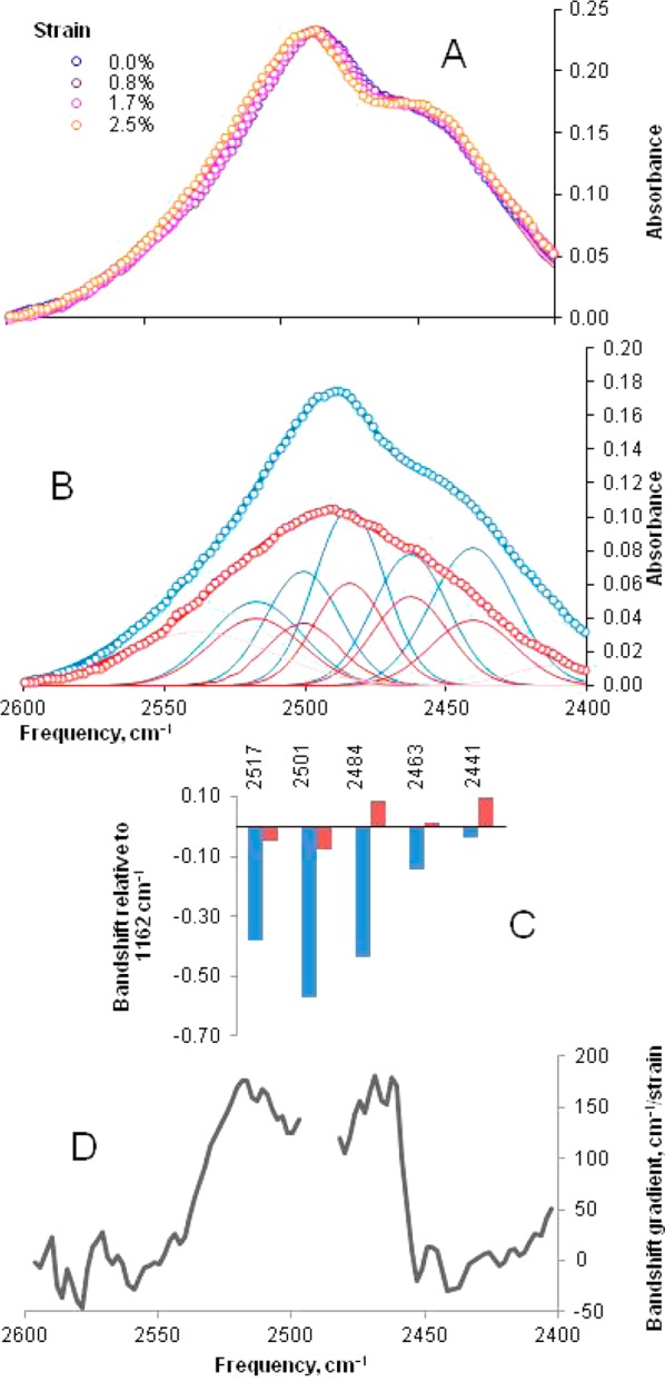
(A) Effect of tensile strain on the longitudinally polarized O–D stretching vibrations of internally deuterated spruce wood cellulose. The O–D stretching regions of the longitudinally polarized (blue) and transversely polarized (red) spectra were deconvoluted (B) into five Gaussian bands (with two additional bands fit to the high- and low-frequency tails). Individual strain-induced bandshifts (C) for the deconvoluted bands (mean of five experiments). Bandshifts for all longitudinally polarized bands were significant (P < 0.05) except for 2441 and 2463 cm–1. Bandshifts for all transversely polarized bands were nonsignificant. (D) Spectral variation in bandshift quantified by the difference integral method. A sharp change in local bandshift occurred between 2460 and 2450 cm–1.
The second approach was to deconvolute the O–D stretching region of the spectrum into individual bands.17 In principle, the number of bands present should be very large, with six crystallographically distinct hydroxyl groups in the unit cell of each allomorph, cellulose Iα and Iβ; two different hydrogen bonding networks for each allomorph; and multiple coupled vibrational modes differing in phase combinations. In practice, the O–D stretching region of the samples after partial internal deuteration was consistent with a preponderance of cellulose Iβ in the A network form, and DFT modeling28 indicates that coupled modes are grouped in frequency with fewer groups than the number of crystallographically distinct hydroxyl groups. Making use of the transversely and longitudinally polarized spectra together as described,17 we were able to obtain a robust separation into five Gaussian bands corresponding approximately to those identified for cellulose Iβ,17 plus two broader bands at 2412 and 2538 cm–1 that probably included both diffuse intensity (the high- and low-frequency tails) and contributions from cellulose Iα and the B hydrogen bond network of cellulose Iβ. Their presence implied that some additional intensity from these other forms of cellulose probably also underlies the rest of the O–D stretching region and complicates the separation into the five bands shown, but modeling further minor bands would have introduced too many adjustable parameters to permit robust fits. Band fitting was done by least-squares minimization using the Solver function in Microsoft Excel. The best-fit band frequencies, widths, and intensities were first calculated for the averaged, normalized spectra from each experiment, and the shifted frequencies for all the bands were then fit for each normalized spectrum while the widths and intensities were held constant. The broad bands at 2412 and 2538 cm–1 were excluded from the statistical analysis. For the remaining deconvoluted bands, bandshifts from five experiments were averaged and significant differences were identified by one-way analysis of variance.
X-ray Diffraction
X-ray diffraction patterns were obtained at ambient temperature and humidity (∼50% relative humidity) using a Rigaku R-axis/RAPID image plate diffractometer. A Mo Kα radiation (λ = 0.07071 nm) source was used, with the beam collimated to a diameter of 0.5 mm.30 Spruce samples ∼0.5 mm thick in the direction parallel to the beam and 2 mm wide were bonded at each end between 0.5 mm aluminum alloy tags using metal-filled epoxy resin, heat-cured for 10 min at 105 °C. The sample was attached at each end to a stretching rig on the goniometer head of the diffractometer, by titanium pins fitted through 3 mm holes in the aluminum tags. The sample was stretched by a M2 machine screw driving a lever arm giving 6:1 leverage. The diffraction patterns were collected from a point close to the fixed end of the sample, normally in perpendicular transmission mode. In principle, tilting experiments are preferred when measuring axial reflections from crystalline fibres. However, the 004 axial reflections from wood cellulose could be readily observed without tilting, and in tilting experiments where this reflection could be measured only at one end of the meridian, its position could not be determined with quite as much accuracy because of small deviations in the centering of the diffraction pattern during each stretching experiment. Both tilting and nontilting modes were therefore used to collect the unit cell dimensions presented here, but only the tilting mode was used to measure any changes in the radial width of the 004 reflection that might indicate a redistribution of stress between microfibrils when the sample was stretched. This was necessary because when the sample is not tilted, a disproportionate fraction of the 004 intensity is likely to be derived from slightly misoriented microfibrils.
Rigaku CrystalClear version 1.4.0 and AreaMax version 1.1.5 (Rigaku Inc., The Woodlands, TX) were used to collect and process images. Each diffraction pattern, corrected for detector geometry but without background subtraction, was extracted in the form of 180 radial profiles each integrated over 2° of azimuthal angle χ.30 To construct difference diffraction patterns, it was necessary first to equalize the rotation and centering of the diffraction patterns by least-squares minimization of differences in the intensity of the 200 reflection between quadrants, using the Solver function in Microsoft Excel.
The positions of the 200, 1–10, and 110 reflections were then determined from the radial intensity profiles averaged over 20° in azimuth. This wide azimuthal distribution was necessary to capture the whole azimuthal range covered by each reflection, because some redistribution of intensity from the wings to the center of the reflection occurred upon stretching as microfibrils realigned toward the strain axis.
Any remaining discrepancies in centering were corrected by averaging the distance from the center (2θ) for each pair of opposite reflections. External calibration of 2θ was checked with LaB6.30
Calculation of the axial (c) dimension of the unit cell was based on 2θ for the 004 reflections, each fitted first in the azimuthal and then in the radial direction as described previously30 using a Gaussian radial profile over a linear local baseline.
The positions of the equatorial 1–10, 110, and 200 reflections were each fit with a linear baseline and an asymmetric function of the form15
where k is a scaling constant, Io is the maximal intensity at 2θ = 2θo, σ is a constant describing the radial width of the reflection, and f(2θ) = 0.3(2θ – 2θo)2 when 2θ < 2θo but zero when 2θ > 2θo. The use of an asymmetric modeled profile allowed closer fits to the data than any symmetric function. The a dimension of the unit cell was calculated directly from the fitted position of the 200 reflection. The b dimension and monoclinic angle γ were then calculated simultaneously from the fitted positions of the 1–10 and 110 reflections, by a numerical adaptation of a method described previously.31 For each experiment, the mean values of a, b, c, and γ were calculated, and hence, the percent deviation from these mean values at each strain level was obtained. This allowed the data from six experiments to be pooled (n = 27), and a, b, and γ were subjected separately to regression against c for the combined data sets.
Tensile Testing
The samples were the same as those used for X-ray diffraction, with aluminum alloy tags at the ends. Load–deformation and stress–relaxation curves were recorded on a Tinius Olsen H1KS testing instrument, correcting displacement of the crosshead for instrumental deflection, and were converted to stress and engineering strain using sample dimensions measured to ±5 μm with a digital micrometer.
Results
FTIR spectra were recorded under tension from thin foils of Sitka spruce wood, less than one cell thick. The wood used was selected for microfibril orientation almost exactly parallel to the grain, maximizing the load carried elastically by the microfibrils and reducing time-dependent deformation during data collection to <10% of the total (Figure 1 of the Supporting Information).
The complex group of O–H stretching bands in the FTIR spectra from wood includes contributions from crystalline and disordered cellulose chains, noncellulosic polysaccharides, and water. Initially, these interfering contributions were removed by vapor-phase deuteration (Figure 2 of the Supporting Information), which substitutes hydroxyl groups on noncellulosic polymers and on some of the surface cellulose chains.15,32 The isotope mass effect moves the O–D stretching bands to a lower frequency by a factor of 1.343. We also used polarized infrared radiation because hydroxyl groups parallel to the fiber axis give longitudinally polarized signals.
The most intense O–H stretching band (or group of bands) remaining after deuteration, the longitudinally polarized band at 3350 cm–1, shifted to a higher frequency (Figure 2 of the Supporting Information) as observed under oscillating stress.32 The shoulder at ∼3280 cm–1, also longitudinally polarized, did not shift.
To simplify the spectra further, we reversed the deuteration experiment, partially deuterating the crystalline interior of the microfibrils under mild alkaline conditions. Accessible hydroxyls then back-exchanged, leaving the internal deuteration stable (Figure 3 of the Supporting Information). The Iβ form of crystalline cellulose with hydrogen bond network A16 predominated in the deuterated fraction, as shown by a strong shoulder at ∼2440 cm–1, the absence of a shoulder at 2420 cm–1, and a low intensity14,17 above 2510 cm–1. Like the O–H stretching band at 3350 cm–1, the corresponding intense, longitudinally polarized O–D stretching band at 2490 cm–1 shifted to a higher frequency under tension and the 2440 cm–1 shoulder did not (Figure 2 and Figure 3 of the Supporting Information).
To take into account some variability between samples in the proportion of the macroscopic strain transferred to cellulose, the longitudinally polarized O–D stretching bandshifts were ratioed against the 1162 cm–1 bandshift, a good indicator of the strain on the cellulose microfibrils32 (Figure 2). Using the difference integral method to quantify bandshifts (Figure 2), a sharp cutoff was evident at 2460 cm–1 between shifting and nonshifting bands. No measurable O–D stretching bandshifts were observed in the transversely polarized spectra (Figure 2).
Thus, it appeared that different hydrogen bonds oriented along the line of tension stretched to different extents. Identifying individual hydrogen-bonded hydroxyls in the FTIR spectra of cellulose is not simple. By combining polarization, internal deuteration, and matching against DFT predictions,15 we concluded that the shifting bands above 2490 cm–1 (Figure 2) corresponded to vibrational modes dominated by O3–D and O6–D stretching. The bands that did not shift, below 2460 cm–1, corresponded to vibrational modes dominated by O2–D and O6–D stretching. Because the O6–D bond is oriented transverse to the fiber axis in predominant hydrogen bond network A,16 the longitudinally polarized spectra had a reduced contribution from the O6–D component. Thus, it was concluded that the O3–D bond was the principal contributor to the deconvoluted bands at 2501 and 2517 cm–1, both of which were shifted strongly in the longitudinally polarized spectra (Figure 2), and the O2–D bond was the principal contributor to the 2441 cm–1 band that did not shift significantly. These data demonstrate that the O3′H···O5 hydrogen bond became longer under strain, while the O2H···O6′ hydrogen bond did not become longer. There are implications for the geometry of the stretching chain.
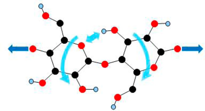
In principle, tension can elongate a cellulose chain, not only by stretching the glucose rings and the glycosidic linkages but also by straightening the zigzag chain conformation in the ring plane. This stretching geometry is consistent with predictions from modeling studies.9,11,12 If each glucose unit pivots on its linkage oxygens O1 and O4 (Figure 3), the O3′H···O5 hydrogen bond should become longer and the O2H···O6′ hydrogen bond shorter.9
Figure 3.

Straightening the kink in the disaccharide unit of cellulose Iβ (origin chain, hydrogen bond network A16). The unstrained form is shown (filled circles) in (a,b) projection in panels A and D. Under tension, the two glucose units (open circles) are rotated in opposite directions through an angle ω around the fulcrum of the glycosidic oxygen (O1, center) (panel A), stretching the O3′H···O5 hydrogen bond by δl = 2h tan(ω), where h is the projected distance from the fulcrum to the midpoint of the hydrogen bond. Panel B shows how the chain length per glucose unit, L (=c/2), then increases by δL = L[cos(10.2° – ω) – cos ω] as the initial kink of 2 × 10.2° in the chain is reduced by 2ω. In panel D, the fulcrum is moved to the midpoint of the O2H···O6′ hydrogen bond, because this hydrogen bond was not observed to undergo a significant change in length. With this geometry, the glycosidic linkage is stretched at the same time as the O3′H···O5 hydrogen bond; i.e., the C1–C4 distance increases at the same time as the O3–O5 distance. With this geometry, it is simpler to calculate δl and δL numerically from the atomic coordinates in the (a,b) projection, and the result is shown for both geometries in panels C and F. The calculation was conducted for both origin and center chains in the cellulose Iβ structure, but the resulting elongation curves for the two chain types were almost superimposed. The leverage ratio is equal to δl/δL.
We found experimental evidence of lengthening of the O3′D···O5 hydrogen bond but not for significant contraction of the O2D···O6′ hydrogen bond. This implies that the chain does become straighter, but simultaneously, the glycosidic linkage itself stretches, canceling out the compression of the O2D···O6′ hydrogen bond. An alternative explanation might be that the pivot point remains at the linkage oxygen but that rotation around the C5–C6 bond allows the length of the O2D···O6′ hydrogen bond to remain constant. However, rotation of C6 would lead to a change in the polarization of the symmetric and antisymmetric C6–H2 stretching vibrations28 at 2840–2850 and 2930–2970 cm–1. No such changes in polarization were observed (Figure 4 of the Supporting Information), suggesting that the effective position of the pivot point is probably not at the linkage oxygen but in the region of the O2D···O6′ hydrogen bond (Figure 3D).
The two-dimensional depiction in Figure 3 is of course simplified: the changes in glycosidic geometry are likely to be more complex than that for which by a simple, unique pivot point can account9,12 because for the projected zigzag angle of the chain to decrease, the glycosidic torsion angles and the C–O–C bond angle must change and these are not coplanar with the figure. Stretching of the monosaccharide rings is also possible, but the extent is predicted9 to be considerably less than the extent of stretching of the glycosidic linkage between them.
Because of its position on the flank of the glycosidic linkage, the O3′H···O5 hydrogen bond is well placed to resist the straightening and consequent elongation of the chain. We can speak of this effect as molecular “leverage” for the hydrogen bond (cf. “atomic levers”33), meaning cooperative action with a fulcrum provided by more rigid covalent bonding. The simplest general way to calculate the effective leverage is from the ratio of the elongation of the O3′H···O5 hydrogen bond δl to the chain elongation per monomer unit δL. These elongations are shown in Figure 3. The leverage δl/δL varies according to the inverse cosine of the angle of rotation. If the fulcrum is at the glycosidic oxygen, the leverage is approximately 4.4. If the fulcrum is at the center of the O2H···O6′ hydrogen bond, the leverage decreases to ∼2.4. This means that the O3′H···O5 hydrogen bond stretches by 2.4 times as much as the monomer length along the chain and is ∼2.4 times as effective in resisting the stretching of the chain as it would be if it were simply stretching in parallel with the covalent linkage and the contributions of the covalent linkage and the hydrogen bond were additive. The leverage is decreased by the slight extensibility of the covalent linkage.
Modeling studies indicate that the O2H···O6′ hydrogen bond is also required for increased chain stiffness.9 Because it does not change significantly in length, it may resist twisting of the chain out of the flat conformation that is optimal for O3′H···O5 hydrogen bonding on the other side of the glycosidic link,9,11 or there may be stereoelectronic synergism along the line of alternating O3′H···O5 and O2H···O6′ hydrogen bonds on the same side of the chain.
This leverage mechanism for the stretching of cellulose leads to the testable prediction that the overall width of the zigzag cellulose molecule will be reduced upon elongation. Because the transversely polarized FTIR spectra gave no evidence that transverse hydrogen bonds between chains underwent changes in length (Figure 2), any change in the overall width of the chains under tension should lead to a reduction in the b dimension of the unit cell (the dimension across a sheet of chains, assuming the cellulose Iβ lattice). Transverse contraction of the unit cell in the a dimension (intersheet spacing) under axial stress has previously been observed,34 but changes were not reported in the b dimension.
To test that prediction, we performed X-ray diffraction experiments under tension (Figure 4), measuring all three unit cell dimensions. There was more stress relaxation than in the FTIR experiments because of the longer duration of the measurement, but approximately half of the applied macroscopic strain was recovered as crystallographic strain, i.e., as an increase in axial dimension c of the unit cell measured from the 004 reflection. This reflection did not become significantly broader under tension (Figure 4), showing that the load distribution between microfibrils remained relatively uniform.
Figure 4.

Tension-induced changes in the X-ray diffraction pattern (A) from spruce wood cellulose. (B) Equatorial intensity profile, measured along the white dotted line in panel A, with the 1–10, 110, and 200 reflections indexed on the cellulose Iβ lattice. (C) Two-dimensional plot of strain-induced intensity changes along the radial profile. Scattered intensity moved from the wings inward toward the center of the equatorial profile (χ = 0) at the same time as the 200 and 110 reflections moved to greater 2θ. (D) Changing position of the axial 004 reflection under tension, without a change in width: blue, zero strain; red, 1% strain.
The associated changes in lateral dimensions could then be deduced from the equatorial reflections, although the deduction was complicated by the increased uniformity of orientation under strain and by the strong overlap between the 1–10 and 110 reflections (Figure 4). The contraction previously observed34 in the a dimension was evident from the outward displacement of the 200 reflection. The overlapped 1–10 and 110 reflections were also displaced outward, and their separation increased.34 This implies contraction of the b dimension across the sheets of chains and an increase in the monoclinic angle as the unit cell became longer (Figure 5). The contraction in the b dimension corroborates the mechanism proposed above.
Figure 5.

(A) Microfibril cross section with the unit cell outlined. The c dimension is perpendicular to the plane of the figure. (B) Strain-induced percentage contraction in transverse dimensions a and b of the cellulose Iβ unit cell and an increase in monoclinic angle γ, for a 1% elongation in axial dimension c of the unit cell. The percentage elongation of the c dimension (crystallographic strain) was calculated from the change in position of the 004 reflection on the fiber axis. The percentage change in dimension a was calculated from the change in position of the 200 reflection, and percentage changes in γ and b were then calculated from the positions of the 1–10 and 110 reflections. Pooled data from six experiments. Percentage changes were significant at the following levels: P = 0.000 (a vs c); P = 0.04 (b vs c); P = 0.004 (γ vs c).
Discussion
The FTIR and diffraction data support a mechanism for elastic extension of the cellulose chain in which much of the additional chain length is obtained by straightening the kink in the chain at each glycosidic linkage.9,12 The FTIR bandshifts show how this straightening of the chain is resisted by the O3′H···O5 hydrogen bond. Just as a rope can be tightened with great force by pulling sideways on its center, this geometry provides leverage for the hydrogen bond in restraining the extension of the chain. The geometry is established by the covalent structure of the glycosidic linkage, but not quite rigidly: the lack of any measurable O2–H stretching bandshift shows that the covalent linkage stretches slightly, slightly reducing the leverage for the O3′H···O5 hydrogen bond. Cooperation of this kind between covalent and hydrogen bonding, to increase the tensile stiffness of a molecule, has not to the best of our knowledge been previously described. It does not lead to the breaking of the hydrogen bond, until the glycosidic linkage itself breaks.
In these respects, cellulose contrasts with spider silk and related strong proteins in which sacrificial hydrogen bonds permit controllable stiffness to be combined with a high fracture energy.35 Molecular leverage has the additional effect of stretching the O3′H···O5 hydrogen bond through a much greater amplitude than the cellulose chain itself stretches, and transverse atomic displacements are also large: the resulting dipolar changes may drive the piezoelectric properties of cellulose, which have been exploited in “smart” cellulose-based devices36 and have unexplored potential as a mechanism for electromechanical signaling in plants.
There is an unexpected qualitative parallel between the crystallographic effects of strain (Figure 4) and the effects of hydration in wood.31 Hydration disrupts intramolecular hydrogen bonding in accessible cellulose chains.37 It also affects stress transmission between fibres, and both mechanisms may contribute to the reduced stiffness of wet wood,31,38 paper, and cotton. The rigidity of cellulose chains in different solvents influences the insolubility of microfibrils and their recalcitrance during biofuel production.39
Isolated cellulose microfibrils have promise for high-performance sustainable nanocomposites.40 To predict the engineering properties of such materials, continuum mechanical modeling needs to be interfaced with molecular-scale modeling: our analysis shows that a classical mechanics approach at the molecular scale can be surprisingly useful if the system is considered as a nanostructure rather than a continuous material and gives direct insight into the molecular origins of Poisson ratios.
The mechanism of tensile deformation described here applies to other polysaccharides sharing the key structural motif of a 1,4′ β-glycosidic linkage flanked by a O3′H···O5 hydrogen bond. In chitin, the most abundant strong polymer in the animal kingdom, the chain conformation required for the O3′H···O5 hydrogen bond is rigidly constrained by intermolecular hydrogen bonding.41 The plant hemicelluloses vary in stiffness, because of partial acetylation on O3 and because they lack the O2H···O6′ hydrogen bond that flanks the 1,4′ β-glycosidic link on the other side.42
The concept of synergism between covalent and hydrogen bonding through molecular leverage in principle can also be applied to other proteins, nucleic acids, and certain synthetic polymers, but in a less simple form. In these polymers, the intramolecular hydrogen bond donor and acceptor atoms are separated by larger numbers of covalent bonds so that the intervening chain segment is less rigid, a single fulcrum atom cannot normally be identified, and larger clusters of hydrogen bonds are likely to act together.43,44 The experimental approach described here, using vibrational bandshifts to follow the stretching of individual hydrogen bonds, should be applicable to other polymers.
Conclusion
We conclude that the stiffness of cellulose is enhanced by hydrogen bonding between O3 of one glucose unit and O5 of the preceding glucose unit. The degree of enhancement is substantially greater than what the hydrogen bond in question would provide without the molecular leverage effect provided by the geometry of the covalent linkage between the two glucose units. That is, the covalent and hydrogen bonding systems work in synergy to enhance the mechanical properties of the cellulose chain.
Acknowledgments
We thank C. Lee and J. Kubicki (The Pennsylvania State University, University Park, PA) for discussions and access to unpublished data. We also thank Y. Nishiyama (CERMAV, Grenoble, France) for critical comments. This work was supported by the Engineering and Physical Sciences Research Council (U.K.), Grant EP/E026583/1.
Supporting Information Available
Supplemental Figures 1–4. This material is available free of charge via the Internet at http://pubs.acs.org.
The authors declare no competing financial interest.
Supplementary Material
References
- Fernandes A. N.; Thomas L. H.; Altaner C. M.; Callow P.; Forsyth V. T.; Apperley D. C.; Kennedy C. J.; Jarvis M. C. Proc. Natl. Acad. Sci. U.S.A. 2011, 108, E1195. [DOI] [PMC free article] [PubMed] [Google Scholar]
- Jarvis M. Nature 2003, 426, 611. [DOI] [PubMed] [Google Scholar]
- Nishiyama Y. J. Wood Sci. 2009, 55, 241. [Google Scholar]
- Diddens I.; Murphy B.; Krisch M.; Mueller M. Macromolecules 2008, 41, 9755. [Google Scholar]
- Nishino T.; Takano K.; Nakamae K. J. Polym. Sci., Part B: Polym. Phys. 1995, 33, 1647. [Google Scholar]
- Saito T.; Kuramae R.; Wohlert J.; Berglund L. A.; Isogai A. Biomacromolecules 2013, 14, 248. [DOI] [PubMed] [Google Scholar]
- Keckes J.; Burgert I.; Fruhmann K.; Muller M.; Kolln K.; Hamilton M.; Burghammer M.; Roth S. V.; Stanzl-Tschegg S.; Fratzl P. Nat. Mater. 2003, 2, 810. [DOI] [PubMed] [Google Scholar]
- Montero C.; Clair B.; Almeras T.; van der Lee A.; Gril J. Compos. Sci. Technol. 2012, 72, 175. [Google Scholar]
- Cintron M. S.; Johnson G. P.; French A. D. Cellulose 2011, 18, 505. [Google Scholar]
- Sturcova A.; Davies G. R.; Eichhorn S. J. Biomacromolecules 2005, 6, 1055. [DOI] [PubMed] [Google Scholar]
- Tashiro K.; Kobayashi M. Polymer 1991, 32, 1516. [Google Scholar]
- Wohlert J.; Bergenstrahle-Wohlert M.; Berglund L. A. Cellulose 2012, 19, 1821. [Google Scholar]
- Salmen L.; Bergstrom E. Cellulose 2009, 16, 975. [Google Scholar]
- Horikawa Y.; Sugiyama J. Biomacromolecules 2009, 10, 2235. [DOI] [PubMed] [Google Scholar]
- Thomas L. H.; Forsyth V. T.; Sturcova A.; Kennedy C. J.; May R. P.; Altaner C. M.; Apperley D. C.; Wess T. J.; Jarvis M. C. Plant Physiol. 2013, 161, 465. [DOI] [PMC free article] [PubMed] [Google Scholar]
- Nishiyama Y.; Langan P.; Chanzy H. J. Am. Chem. Soc. 2002, 124, 9074. [DOI] [PubMed] [Google Scholar]
- Sturcova A.; His I.; Apperley D. C.; Sugiyama J.; Jarvis M. C. Biomacromolecules 2004, 5, 1333. [DOI] [PubMed] [Google Scholar]
- Liang C. Y.; Marchessault R. H. J. Polym. Sci. 1959, 37, 385. [Google Scholar]
- Marechal Y.; Chanzy H. J. Mol. Struct. 2000, 523, 183. [Google Scholar]
- Sugiyama J.; Persson J.; Chanzy H. Macromolecules 1991, 24, 2461. [Google Scholar]
- Fengel D. Holzforschung 1992, 46, 283. [Google Scholar]
- Hinterstoisser B.; Salmen L. Cellulose 1999, 6, 251. [Google Scholar]
- Kokot S.; Czarnik-Matusewicz B.; Ozaki Y. Biopolymers 2002, 67, 456. [DOI] [PubMed] [Google Scholar]
- Ivanova N. V. Zh. Prikl. Spektrosk. 1989, 51, 301. [Google Scholar]
- Gritsan V. N.; Zhbankov R. G.; Kachur V. T. Acta Polym. 1982, 33, 20. [Google Scholar]
- Gardner K. H.; Blackwell J. Biopolymers 1974, 13, 1975. [DOI] [PubMed] [Google Scholar]
- Nishiyama Y.; Sugiyama J.; Chanzy H.; Langan P. J. Am. Chem. Soc. 2003, 125, 14300. [DOI] [PubMed] [Google Scholar]
- Lee C. M.; Mohamed N. M. A.; Watts H. D.; Kubicki J. D.; Kim S. H. J. Phys. Chem. B 2013, 117, 6681. [DOI] [PubMed] [Google Scholar]
- Sturcova A.; Eichhorn S. J.; Jarvis M. C. Biomacromolecules 2006, 7, 2688. [DOI] [PubMed] [Google Scholar]
- Thomas L. H.; Altaner C. M.; Jarvis M. C. J. Appl. Crystallogr. 2013, 46, 972. [Google Scholar]
- Zabler S.; Paris O.; Burgert I.; Fratzl P. J. Struct. Biol. 2010, 171, 133. [DOI] [PubMed] [Google Scholar]
- Hofstetter K.; Hinterstoisser B.; Salmen L. Cellulose 2006, 13, 131. [Google Scholar]
- Marszalek P. E.; Pang Y. P.; Li H. B.; El Yazal J.; Oberhauser A. F.; Fernandez J. M. Proc. Natl. Acad. Sci. U.S.A. 1999, 96, 7894. [DOI] [PMC free article] [PubMed] [Google Scholar]
- Nakamura K.; Wada M.; Kuga S.; Okano T. J. Polym. Sci., Part B: Polym. Phys. 2004, 42, 1206. [Google Scholar]
- Keten S.; Xu Z.; Ihle B.; Buehler M. J. Nat. Mater. 2010, 9, 359. [DOI] [PubMed] [Google Scholar]
- Csoka L.; Hoeger I. C.; Rojas O. J.; Peszlen I.; Pawlak J. J.; Peralta P. N. ACS Macro Lett. 2012, 1, 867. [DOI] [PubMed] [Google Scholar]
- Bergenstrahle M.; Wohlert J.; Himmel M. E.; Brady J. W. Carbohydr. Res. 2010, 345, 2060. [DOI] [PubMed] [Google Scholar]
- Obataya E.; Norimoto M.; Gril J. Polymer 1998, 39, 3059. [Google Scholar]
- Rabideau B. D.; Agarwal A.; Ismail A. E. J. Phys. Chem. B 2013, 117, 3469. [DOI] [PubMed] [Google Scholar]
- Klemm D.; Kramer F.; Moritz S.; Lindstrom T.; Ankerfors M.; Gray D.; Dorris A. Angew. Chem., Int. Ed. 2011, 50, 5438. [DOI] [PubMed] [Google Scholar]
- Nishiyama Y.; Noishiki Y.; Wada M. Macromolecules 2011, 44, 950. [Google Scholar]
- Scheller H. V., Ulvskov P., Merchant S., Briggs W. R., Ort D., Eds. Hemicelluloses; Wiley: New York, 2010; Vol. 61, p 263. [DOI] [PubMed] [Google Scholar]
- Bosaeus N.; El-Sagheer A. H.; Brown T.; Smith S. B.; Akerman B.; Bustamante C.; Norden B. Proc. Natl. Acad. Sci. U.S.A. 2012, 109, 15179. [DOI] [PMC free article] [PubMed] [Google Scholar]
- Livesay D. R.; Huynh D. H.; Dallakyan S.; Jacobs D. J. Chem. Cent. J. 2008, 2. [DOI] [PMC free article] [PubMed] [Google Scholar]
Associated Data
This section collects any data citations, data availability statements, or supplementary materials included in this article.