Abstract
A skin conductance monitoring system was developed and shown to reliably acquire and record hot flash events in both supervised laboratory and unsupervised ambulatory conditions. The 7.2 cm × 3.8 cm × 1.2 cm monitor consists of a disposable adhesive patch supporting two hydrogel electrodes and a reusable, miniaturized, enclosed electronic circuit board that snaps onto the electrodes. The monitor measures and records the skin conductance for seven days without external wires or telemetry and has an event marker that the subject can press whenever a hot flash is experienced. The accuracy of the system was demonstrated by comparing the number of hot flashes detected by algorithms developed during this research with the number identified by experts in hot flash studies. Three methods of detecting hot flash events were evaluated, but only two were fully developed. The two that were developed were an Artificial Neural Network and a Matched Filter technique with multiple kernels implemented as a sliding form of the Pearson Product-Moment Correlation Coefficient. Both algorithms were trained on a “development” cohort of 17 women and then validated using a second similar “validation” cohort of 20. All subjects were between the ages of 40 and 60 and self-reported 10 or more hot flashes per day over a three day period. The Matched Filter was the most accurate with a mean sensitivity of 0.92 and a mean specificity of 0.90 using the data from the development cohort and a mean sensitivity of 0.92 and a mean specificity of 0.87 using the data from the validation cohort. The Matched Filter was the method implemented in our processing software.
Keywords: Hot flash, hot flush, miniature recorder, ambulatory monitor, template matching, matched filter, electrode, hydrogel, Pearson, correlation, neural network
1. Introduction
A hot flash event is the sudden onset of intense flushing in the upper torso and face, often followed by profuse sweating and chills (Kronenberg 1990). The etiology of hot flashes is thought to be related to episodic abnormalities of thermoregulation associated with changes in hormone levels that occur at menopause, but the mechanism is not clearly understood (Low et al 2011). There are about 42 million American women between the ages of 45 and 65 years (U.S. Census 2012 Statistical Abstract). At least two thirds of these women will experience hot flashes and approximately 20% will seek medical treatment for debilitating symptoms (Kronenberg 1990).
As reflected in NIH-sponsored seminars (Women's Health Seminar Series 2010), and numerous conferences on menopause there is intense interest in the research community regarding the etiology of hot flashes and in finding effective and safe non-hormonal treatment. However, research is currently hindered by the lack of a feasible, reliable and accurate objective measure of hot flash occurrence. Most studies currently use a 7-day self-reported hot flash diary. (Sloan et al 2001). This measure is subjective and can be inaccurate and unreliable because participants may forget or fail to enter hot flashes in the diary (especially at night when many hot flashes occur), and the exact timing of the hot flash typically is not recorded (Miller and Li 2004). In addition, keeping a daily diary is labor intensive and inconvenient.
Based on input from symptomatic women and experienced investigators, the requirements for a good hot flash monitoring system were clear. The aim of this study was to develop a miniature, wireless device that would be reliable, user-friendly, accurate, and could collect data for up to seven days under ambulatory conditions. The monitor would need to collect data during waking and sleeping hours, without interfering with daily activities. This also necessitated the development of an electrode that would provide artifact-free signals with little or no baseline drift. Such a device could be used to record hot flashes under ambulatory conditions in clinical studies of various drugs and other therapies.
2. Methods
2.1 Miniature ambulatory hot flash monitor
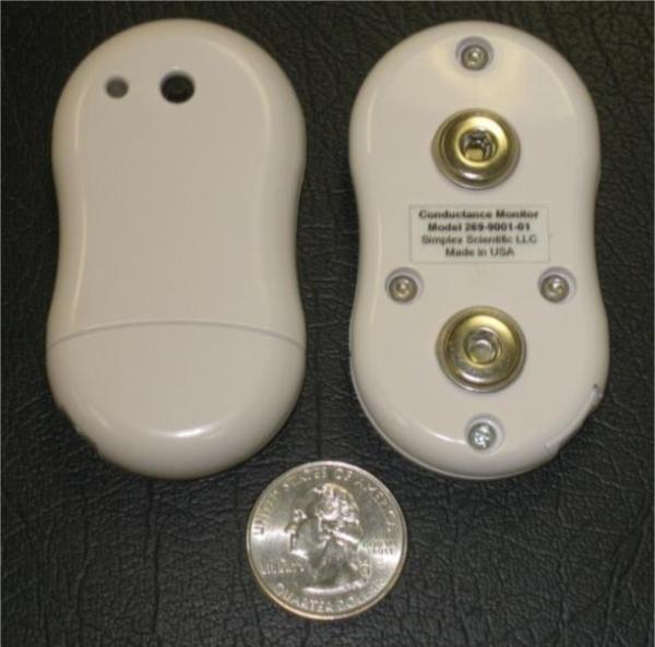
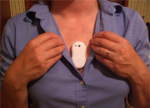
We developed a commercial hot flash monitoring system that included a monitor and the software to upload and process the data. The monitor is the first to collect data on skin conductance without wire leads from ambulatory research subjects for up to seven days. The monitor clips directly onto the self-adhesive electrode patch eliminating the need for any cables. It is worn unobtrusively on the sternum hidden under clothing and is easy to remove and replace. The housing of the monitor is not water resistant so when bathing the monitor is unclipped from the electrode, which is left in place. After bathing the electrode patch is simply patted dry and the monitor reconnected. Figure 1 shows the front centered push button to record perceived hot flash and the offset LED where a green flash every 5 s indicates recording and a red flash indicates button pushed. The two snaps on the back connect directly to the electrode patch. Figure 2 shows how the monitor is worn.
Figure 1.
Front and back of the monitor. The size of the monitor is 7.2 cm × 3.8 cm × 1.2 cm and it has a mass of 16 g (0.56 oz) including the battery. The battery has a life of more than 1 week. The conductance range is 0 to 30 μS.
Figure 2.
Commercialized Hot Flash monitor. Placement of the monitor is usually done vertically over the sternum but it can also be placed on either side.
2.2 Hot flash events as measured by skin conductance
Autonomic temperature regulation in humans employs vasodilatation and sweating to cool the body. An increase in sternal skin conductance due to sweating has been shown to be an accurate measure of the occurrence of hot flashes in temperature-controlled laboratory settings (Low et al 2011. Molnar (1975) demonstrated that the skin temperature of the upper anterior torso increased during a hot flash event, accompanied by sweating. Thus, the upper torso was chosen as the best place to monitor skin conductance and the sternum was chosen because it was easy to affix electrodes and the monitor was less likely to interfere with daily activity. During our research we made no attempt to place the electrodes on other areas of the torso or on any of the extremities.
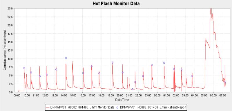
We observed (average of 360 hot flashes) that the hot flash conductance response takes approximately 1 to 2 min to go from its baseline to its peak. It then takes 5 to 10 min for the response to return back to the baseline. Figure 3 shows the skin conductance record from a typical subject. The biphasic response that occurred during the return to baseline was found in approximately 15% to 20% of the hot flash waveforms that were collected during this research. No explanation as to what caused this could be found in the literature or could the cause be determined during this research.
Figure 3.
A sample of raw data collected by the new monitor. The hot flash events can be clearly seen with the blue circles showing where the subject marked the data when experiencing hot flash symptoms. The large event near the end of the trace shows the effects of exercise.
The portion of the hot flash conductance signal that has the highest frequency component is the rise time and takes place in 1 to 2 min. With this information it was decided to sample once every 10 s which easily met the Nyquist sampling criterion. Sweat duct activity is initiated and modulated by body temperature, hormones, and neural activity. Sweat is generated in the sweat glands and carried to the surface through the sweat ducts. The hot flash response (increased conductance) is a combination of the open sweat pores and the sweat on the surface of the skin. Conductance was calculated by applying a small voltage of 0.5 V to the surface of the skin using a pair of closely spaced electrodes (3cm in our studies) and measuring the resultant current flow through a fixed reference resistor. To prevent electrode polarization, two voltage pulses were used with one having a positive polarity and the second with a negative polarity and spaced 5 s apart. Both pulses had duration of 240 ms, which is approximately five times the time constant of skin when stimulated by an electrical signal. The conductance calculated from the two pulses was averaged to produce the sample and stored in memory.
The hot flash conductance is typically 5 to 10 times larger than the baseline conductance and roughly proportional to the cross-sectional area of the electrode interface. There is also a surface leakage current due to the layer of sweat on the skin below the electrode. The three most important characteristics of hot flash skin-conductance events are the rapid rise in the conductance, the characteristic peak, and the exponential-like fall. These characteristics were the most useful in detecting a hot flash event in conductance data.
2.3 Electrode design
We began with an isotonic sodium chloride-based semi-liquid gel that approximates sweat (0.1 to 0.3% NaCl). This gel was substituted for the higher salt content (~5% NaCl) gel and sponge in a standard ECG electrode. These modified electrodes had a number of major limitations. The gel between the skin and the electrode migrated at times causing the conductance to drift without physiological involvement. A second major limitation was that the impermeable plastic patches containing the semi-liquid gels trapped sweat under the electrode increasing hydration causing a continual rise in conductance over time thus rendering the electrode essentially useless after a few days of use. A third problem was that the stickiness or tack was designed for a few days of use and is very aggressive often leaving a large welt on the skin after removal.
Jossinet and McAdams (1990) showed that electrodes using semi-liquid gels as the skin-electrode interface, keep the skin well hydrated and skin resistance decreases (conductance increases) with time. They also showed that for hydrogel electrodes, skin resistance does not decrease with time because these materials do not actively hydrate the skin. Their investigations demonstrated that skin conductivity is best measured using a hydrogel (or very mild wet gel) electrode interface. Hydrogels are water-containing polymers that incorporate either natural or synthetic hydrocolloids and are therefore “solid” and hydrophilic.
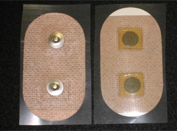
There are many manufactures of hydrogel materials and there many types of hydrogel materials. We decided to acquire hydrogel samples from AmGel, Inc. a major manufacturer of medical hydrogel materials. Samples were chosen from three of AmGel's major hydrogel Series and included AG603, AG703, and AG803. Samples in the AG900 series were not chosen because of the high volume resistivity of that material. Figure 4 shows the hydrogel materials that were cut into 1.5 cm2 squares and placed in pairs on a 4 cm by 7 cm oval skin-colored polyester containing two pre-assembled Ag/AgCl metal electrodes.
Figure 4.
An assembled hydrogel electrode patch used during early experimentation to provide data on hydrogel formulations. The design uses spunlaced polyester coated with an acrylic adhesive, Ag/AgCl metal electrodes with snaps on the back, and a special formulated hydrogel metal-to-skin interface.
Selection of the hydrogel material was based on optimizing low baseline values, low baseline drift, and signal-to-noise ratios when measuring hot flash episodes. The AmGel AG703 and AG803 adhesive hydrogels were found to be superior to AG603 hydrogel, BIOLOG gels, or 0.1% or 0.9% saline in hydrogels. The best overall results were obtained using AG803 which is a specially formulated hydrogel material usually used for electrophoresis. The patch material is spunlaced polyester (MacTec, Inc - TM-9478). The patch is coated on one side with 594 acrylic-based hypoallergenic pressure-sensitive adhesive. The adhesive material is a medical grade adhesive and is formulated for sustained contact with human skin. It is protected by a 70# dense, semi-bleached Kraft release liner. The TM-9478 material is designed for use as a breathable medical tape. The hydrogel and the polyester absorb the sweat from the skin and the breathable feature allows the sweat to evaporate. This prevents the accumulation of sweat and provides for a low amplitude base line that does not wander over time. The baseline conductance changed a few MicroSiemens over the 3-day testing periods usually increasing in magnitude. This was assumed to be caused by the accumulation of salt content under the electrode. If the electrode patch became wet as in taking a shower, it dried in about 30 m and was ready to continue collecting hot flash data. Removal of the electrode after a week caused mild skin irritation similar to that caused by the removal of a Band-Aid. Subsequent electrode application was on a new skin site.
2.4 Subject selection and experimental protocol
Inclusion/Exclusion criteria: Women recruited were between the ages of 45 and 60, reported having 10 or more hot flashes per day over a three day period), had no known allergy to adhesive or tape, and had not had a menstrual period in the past 6 months. To avoid potential problems with the low voltage device, we excluded women who had pacemakers, implantable defibrillators, and those who planned to travel by air during the study. There was no restriction on use of concurrent medications.
Having limited funds we were forced to limit the size of the human studies. Individuals were chosen to best represent the demographics of an ‘average’ subject. A “development” cohort of 17 women was enrolled as well as a “validation” cohort of 20 women. The mean daily HF # was 9.0 (SD 5.2). Participants wore the miniature monitor continuously for 7 days. In addition, each participant kept a daily diary in which she was asked to record the exact time of each hot flash. We asked participants to keep the diary only for the first 3 days of monitor recording to maximize the accuracy of self-report and minimize participant burden. After 3 days subjects were less likely to mark hot flash events even though the waveform morphology matched the data taken during the first 3 days.
At the clinic, each participant signed the IRB consent form, a hot flash monitor was applied near the sternum because motion artifact is minimal at this location, and the participant was instructed in use and departed the clinic. The subject was instructed to mark hot flashes, unsnap the hot flash monitor during showering, and then snap it back onto the electrode. She returned after 7 days and the hot flash monitor was connected to a computer for downloading the 7-day data.
2.5 Data processing and algorithm development
During hot flash events the skin conductance rises rapidly as the sweat ducts open and begin exuding sweat. The conductance reaches a peak and then falls slowly as the as the sweat evaporates from the electrode. This morphological shape varies somewhat in rise time, height, width, and fall time within and across subject records. The hot flashes have a rise time of approximately 1 to 2 min and duration typically of no more than 10 min. The task was to locate the hot flashes events in the data among motion artifacts such as those produced by exercise.
Because the skin conductance data usually contained artifacts and noise and often had a slow drift, the data were first filtered with two separate filters. The noise was minimized without significant distortion by using a moving average convolution filter with a width of 13 points (±1 min). To minimize the baseline drift in the data, they were then filtered using a 361 point (±30 min) median filter. This type of filter has the characteristic of eliminating drift without distorting the sharp peaks. Since the data were post-processed using stored data, it was possible to use centering on both filters to eliminate all phase shift error. This is done by passing the filter kernel over the data in one direction and then in the other, doing half of the required calculations in each of the two directions.
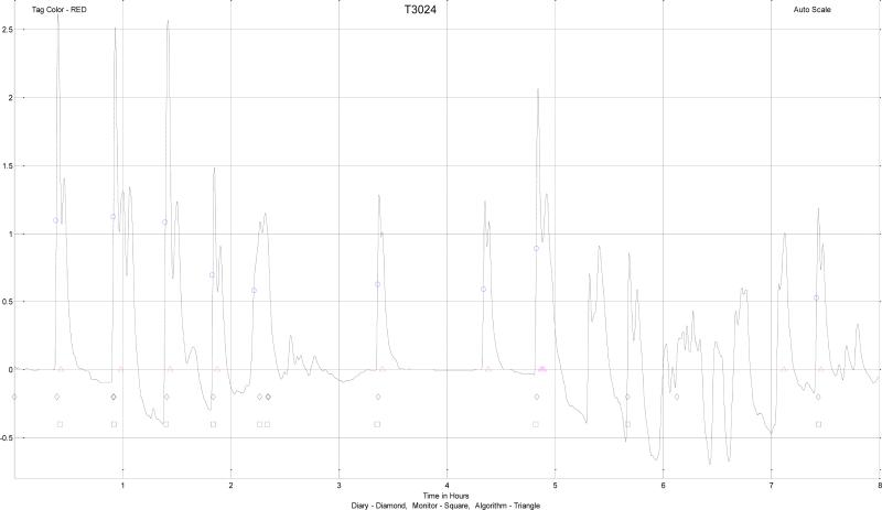
We found the event marker or the subject diary did not yield a sufficiently reliable set of hot flashes from which to develop an algorithm. In the laboratory, subjects marked the data consistent with the appearance of a hot flash event. In ambulatory conditions this was not always the case. Subjects would often indicate that a series of hot flashes had occurred in agreement with the monitor. Then they would miss one or more events with similar wave shapes, amplitudes, and durations in the local neighborhood. We assumed that the subject simply had not marked these events. To provide a “gold-standard” of hot flash waveforms for the purpose of developing an algorithm we needed to have data/waveforms of essentially unequivocal hot flashes. In the service of this end, five experts who already had extensive experience with hot flash data or who were trained in viewing skin conductance tracings, were asked to mark what were to them, unequivocal hot flashes, or those they were sure were hot flashes from the development set as shown in figure 5. The experts used the characteristic rapid rise in the conductance terminating in a peak and the exponential-like fall within a 10 min window to score the data. These characteristics were the most useful in detecting hot flash events in conductance data. Those marked by the majority of the experts were considered to be the “gold standard” hot flashes for the purpose of algorithm development.
Figure 5.
Hot flash data that has been smoothed by a moving average filter and with baseline restoration using a median filter. Shown are subject (written diary – ◇, pushed the button on monitor – □), expert ( ), and algorithm (
 ), marked hot flash events. The ordinate is scaled in μS.
Three methods of detecting hot flash events were evaluated, but only two were fully developed. One method selected known hot flash events from the development data set and averaged these data producing one or more representative patterns. The patterns could then be matched to the data using statistical methods. This method performed less well than the other two methods and was subsequently discarded.
A second method was a parameterized model where the shape of the model could be altered by modifying the model parameters to match the shape of known hot flash events. The log-normal function was chosen as the model because of its shape and the Pearson Product-Moment Correlation Function was chosen to determine goodness-of-fit of the kernel. This method is known as a matched filter and proved to be the most accurate of the three.
A third method used an algorithm that could learn the shape of a true hot flash event using samples of known hot flash events from the development data set. We used an Artificial Neural Network, a mathematical model that simulates the neuron by multiplying the inputs to the network using a series of weights and then sums these weights to produce a single result that is either true or false. During development, the weights are adjusted to obtain the best accuracy.
2.6 The matched filter
Hot flash events have a shape that can be recognized as similar to a constant with a squared exponent that is skewed to the right. There are many functions with this characteristic but it was decided to limit the search to the Poisson distribution and the log-normal distribution since they are well known. Even though these functions are considered probability density functions, it is possible to convert them to functions of time or position using a substitution of variables. Using the Poisson distribution function the variance and the mean are equal in all cases. This makes it difficult to alter the rise time, width, and fall time independently as was needed, so this approach was discarded.
The log-normal function is useful in modeling naturally occurring variables that are the product of many independent variables rather than the sum of these variables. Since the hot flash event is modulated by body temperature, hormones, and neural activity this function seemed to be a natural fit. The equation for the one dimensional log-normal function is shown in equation (1).
| (1) |
The symbol σ is the standard deviation and the square σ2 is the variance. The symbol μ is the mean value and the x symbol is the independent variable and can range from –∞ to +∞. The term in front of the exponential is the normalization constant and comes from the fact that the integral over the exponential function is not unity but rather . What was needed was an equation that had a similar shape but where the mean and standard deviation could be replaced with characteristics of the hot flash curve, such as center and width. An empirical equation was developed using the log-normal as a model and is shown in equation (2).
| (2) |
The term x is the independent variable and has a range from 0 to 90 since the data were sampled and stored every 10 s the range spans [90 * 10/60] or 15 min. The 10 s interval was chosen because that was fast enough to capture the fastest component of the signal (the rise) without loss of information.
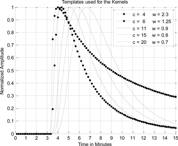
The term center is where the peak occurs and the width is a measure of the width and skew or drop in the tail. The offset term is the amount of time from zero to where the function's rising edge begins since there is usually a flat baseline just before the rise. It was readily determined that the slope of the rising edge, the width of the kernel, and the length of the tail were the most important parameters. The variables center and width in equation (2) were chosen to produce the best statistical results when compared with experts who marked the data sets for true hot flash events. Initially, it was hoped that a single pattern or kernel could be developed with fixed constants for the center and width that could be used for all subjects. However, we found better hot flash detection accuracy when five separate kernels all with unique values for the center and width were used as shown in figure 6.
Figure 6.
The five templates used for the kernels, where c is the center parameter and the w is the width parameter.
The kernels were correlated with the data one session at a time (all of the records) by sliding the kernel along the data taking one sample point at a time and using the Pearson Correlation Coefficient (PCC) to determine how well the kernel and the data matched. We used Receiver Operating Characteristic (ROC) curves to determine the best PCC. ROC curves plot the sensitivity (percent of positive values correctly identified) by 1 – specificity (percent of negative values incorrectly identified). PCC values of 85% or greater was determined to be the optimal cutoff value for detecting a hot flash.
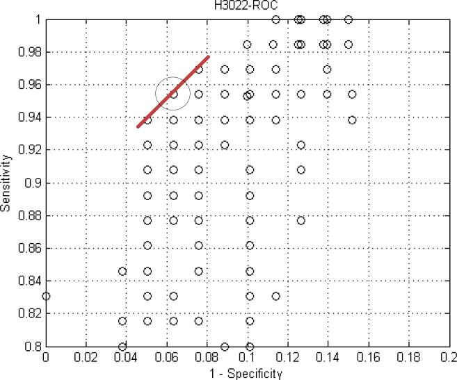
The Pearson Product-Moment Correlation Function was implemented in MatLab© as a sliding or moving algorithm and this was used to determine the best values for the center and width parameters. Extensive use was made of Receiver Operating Characteristic (ROC) curves to determine what values to use for the center and width for the parameterized kernels. Figure 7 shows an example of one of these curves.
Figure 7.
A ROC curve for subject 3022 shows the results of scanning the parameters for the kernel. Each data point represents the results of processing the data with a fixed center and width. The circled data point is where the optimum value for width and center occurred.
ROC curves were run for each of the 17 subjects. We tested a range of values for one variable of the kernel, say width, while holding center constant. For every value tested, we calculated an average sensitivity and 1 – specificity for the cohort. We plotted average sensitivity and 1 – specificity for each width value in the range tested. The result is one ROC curve for say width 5 to 15, center equal to 11. Then we scanned the width again with center equal to 15 and plotted these data on the same graph. This process was repeated for all of the center values. The center and width values that generated the point in the upper left hand corner were the optimal values for the two variables.
2.7 The artificial neural network
An adaptive neural network is a method of identifying patterns in new observations where the identity of these patterns has been learned on the basis of a training set containing a subset of these observations and where the groupings of these patterns has been previously established. This method was originally developed in the 1940s by McCullough and Pitts. They built a mathematical model that simulated the biological neuron by multiplying the inputs to the network with a series of weights and then summing these values to produce a single output that is either true or false. This is similar to how the dendrites and axons function in our brains. The signals entering the dendrites of a neuron are modified by various chemical and electrical processes before being summed and sent along the axon where the signal is presented to other neurons.
Modifications of the input signals are done continously as the biological system adapts to various local and external stimuli. The neural network uses weights to modify the input signals, but only does this during a training session and usually does not modify these weights when the neural network is used to classify signals. In a neuron the connection to the dendrite can be either excitatory or inhibitory while in the artificial neural network this is accomplished using weights that are numbers less than one and can be either positive or negative. The classifications are determined by using quantitative information that describes various implied traits or characteristics. The neural network is presented with individual training patterns along with the classification information describing to which group the pattern belongs. Part of the learning process is to determine which of the traits or characteristics are important to the classification process using arrays of weighting coefficients. This type of identification is called a statistical classification since the classification will show a variable behaviour that is statistical in nature, and when accomplished using machine learning it is often called supervised learning.
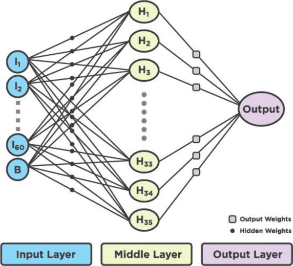
We used a common form of the neural network with an input layer, a hidden layer and an output layer. The name usually given to such a network is the perceptron (Rosenblatt 1958). The artificial neural network had an input layer containing 60 nodes of hot flash data and 1 bias node. The hidden layer contained 35 nodes and the output node contained one node. Figure 8 shows an example of an artificial neural network.
Figure 8.
The signal flow diagram of the artificial neural network used in this research.
The size of the input was chosen to be 60 nodes because this represented a 10 min sample of a hot flash event using a 10 s sampling rate. The predominant features of the rapid rise, smooth peak at the top, and the exponential-like fall of the tail all occur within this 10 min window. A 61st node was added to the input to act as a bias term since the output will have values between 0 and 1 rather than the usual ±1. The 30 nodes in the hidden layer were chosen empirically using the literature as a guide (Semlow 2009, Smith 2003). They suggest using fewer hidden nodes than there are in the input. Hidden node sizes between 20 and 60 were evaluated and a value of 35 was chosen because it provided sufficiently good results without requiring lengthy computation times. An equation that describes the neural network process is:
| (3) |
Where x is the input symbol, w is the multiplier weights, is the input sample number, b is a bias term, N is the total number of inputs, and a is the output or activation. The output a is often passed to a nonlinear discrimination or activation function with an output of ±1, 0 to 1, or some nonlinear mathematical function. There are a number of such discriminator functions each with its own special characteristics including a vertical line with a range from 0 to 1, a sloped line, the hyperbolic tangent, and the sigmoid function. The sigmoid is usually the function of choice because it is a monotonic function and has the ability to compress the output giving its networks greater stability.
The sigmoid also happens to be a differentiable function where the derivative is easy to calculate.
| (4) |
| (5) |
For the purposes of this research the sigmoid abscissa was scaled to ±1 and the ordinate for the sigmoid derivative was scaled to 0 to 1. This normalization may not have been necessary, but doing so is the best way of keeping the results of calculations near zero and thus provides the best dynamic range using a digital computer. Neural network training is accomplished by changing the weight values using some algorithm with an error function that is the difference between the output value from the network and the desired value for a given input.
| (6) |
| (7) |
| (8) |
If the equations were used in the form shown above, the solution would most likely overshoot and oscillate, or in the worst case diverge. To remedy this, learning constant α is used to control the speed of convergence. The equations are modified as follows:
| (9) |
| (10) |
The constant α is chosen empirically and is always less than one usually in the range between 0.1 and 0.00001. The greatest effort comes in defining the training data set and in the actual training of the neural network. The training is done by submitting patterns that should elicit a true response along with an indication that the pattern is true and patterns that elicit a false response along with the indication of being false. This training is usually done with hundreds of such patterns and then retrained with the same patterns a few hundred times. A group of such training patterns is called an epoch and if too many epochs (>1000) are used for training, the neural network can become over-trained. Should this happen, the development set will have excellent statistics and any evaluation set will have very poor statistics. The idea is to train with just enough epochs such that both sets have similar statistical outcomes.
The training process begins by setting each of the weights to a small random value, usually in the range between 0.01 and 0.0001. The choice of range is purely empirical and there are no hard and fast rules to follow. We used a flat probability density function (pdf) with numbers between ±0.01. The shape of the pdf and the values were an empirical choice. For the actual training, input data are presented to the input of the network and multiplied by the weights producing an output. The forward process produces discriminator values for both the hidden and output layers that are actually classification probabilities between 0 and 1. Once an input pattern has been processed in the forward direction all of the values for the hidden and output layers are known as well as the weights for both layers.
A process called back propagation is then used to do the actual training. The fastest way to train a neural network is to use the gradient method to modify the values of the weights. This method is often called the method of steepest descent or the delta rule. The gradient method changes the network's weights and bias so that the error proceeds towards a minimum along the steepest gradient. The gradient descent method is similar to the least mean squares algorithm used in adaptive filtering. The first step is to use the classification probabilities and calculate their first derivatives using equation (5). The second step is to compare the desired output value with the network output value using equation (6) creating an error term err. The output value from the network will be between 0 and 1. If the value is close to the desired value the error term will be close to zero and the first derivative will also be near zero. In these cases the weights in the various layers should not be changed or only changed by a small amount. On the other hand, if the error term is large, the weights should be changed by an amount that takes into account both the sign and the magnitude of the error term. A mathematical description describing the slope for output Wo(0) weight with everything else held constant can be written as:
| (11) |
The term “slope_output” describes how much the output will change with a change in the sum of the values from the hidden layer after the respective output weights have been applied. To find the slope of the hidden weights a similar analysis can be used and found by:
| (12) |
The variable dhdw is multiplied by the learning constant mu and the error err and the results are used to find new values for the hidden weights.
A similar process is carried out for the output weights. The error for each input pattern is squared and added to the sum of the pervious squared errors. When an epoch is completed the square root is taken of this sum and used as a measure of how well the network is converging and displayed on the system console.
The neural network software was implemented in MatLab and the size of the hidden layer could be changed by modifying a constant. The output layer only needed one node with a value of 1.0 if a hot flash event was present and a value of 0.0 if no hot flash event was present. Values in between these indicated the probability of an event being a hot flash or not.
3. Results
Ambulatory monitors used to detect hot flashes have typically been large, are contained in a case over the shoulder or on a vest and encumbered with wires. We developed a commercial hot flash monitoring system that includes a monitor, electrodes, and the software to upload and process the data. The monitor is the first to collect data on skin conductance wirelessly from ambulatory research subjects for up to seven days. The monitor clips directly onto the self-adhesive electrode patch eliminating the need for any cables. It is worn unobtrusively on the sternum hidden under clothing and is easy to remove and replace.
Our optimized parameterized kernels of our matched filter produced the best results with a mean sensitivity of 0.92 and a mean specificity of 0.90 using the development cohort. Using the same algorithms on the validation cohort of 20 individuals produced an average sensitivity of 0.92 and the average specificity of 0.87. Using the neural network algorithm the results were not as good. With the development cohort the neural network produced a mean sensitivity of 0.93 and a mean specificity of 0.89. The results from the validation cohort of 20 individuals had a mean sensitivity of 0.87 and a mean specificity of 0.84. The detailed tabulated results from both algorithms can be found in the PhD Thesis in the references (Bahr 2012).
4. Discussion
Over the past 40 years, skin conductance has emerged as the physiological gold standard for the objective measurement of hot flashes in an ambulatory setting. In the 1970s and 1980s many physiological parameters were monitored in laboratory studies of hot flashes (Tataryn et al., 1979, Kronenberg et al, 1984, Freedman 1989). These included several peripheral sites for measurement of skin temperature, skin blood flow, heart rate, skin conductance and core temperature. However sternal skin conductance became the measure of choice and most valid physiological measure of hot flash occurrence due to the relatively clean nature of a distinctive waveform compared with far greater variability in other physiological signals. This is especially valuable outside of laboratory settings.
The most widely used research tool for measurement of hot flashes, self-report in a diary, has reliability issues, as does the use of electronic event markers. (Freedman 2001, Carpenter et al, 2004, Mann and Hunter 2011). And while in the laboratory there is very good correlation between physiological measures and self-reported hot flashes (Tataryn et al 1981; Meldrum et al 1979,, Kronenberg et al 1984), outside of laboratory settings, reported concordance between skin conductance and self-report varies greatly (Freedman 1989, Carpenter et al 2004, Mann and Hunter 2011). This is likely due 1) to the fact that skin conductance is only one aspect of the physiology of a hot flash, 2) to variable environmental conditions, and 3) that tracings obtained in free living people at times have areas of poor data quality (Carpenter et al, 2012). Thus, no one physiological measure will be the perfect objective measure of hot flashes.
NIH's desire for skin conductance monitors was that they provide data while subjects maintained daily activities (Miller 2004). So our focus was on skin conductance and in developing a miniaturized, wireless, easy to use monitor. Knowing that a hot flash generates a particular skin conductance response, and from the literature, that clear skin conductance signals can be seen during sleep, even when the subject does not awaken to report them (Kronenberg 1990), we used the skin conductance signal to extrapolate to other times when the data clearly showed a response but with no associated subject report. This was for the purpose of developing an algorithm that would more accurately identify hot flashes. We did this by using experts who included experienced hot flash researchers and others who were familiar with our monitor and the hot flash waveform it produced, to identify skin conductance wave forms most likely to be hot flashes. These were then be used to develop an algorithm to detect these patterns.
Carpenter and colleagues (2012) compared the Biolog (standard in the field), with the Freedman hygrometry ambulatory monitor (2007) and a prototype of the Bahr monitor (Webster et al, 2007) with the first iteration of the detection software, not then commercially available because it was a preliminary algorithm. They reported that more hot flashes were detected by the Bahr monitor than the subject reported. This was partially due to the fact that the first iteration of the hot flash detection algorithm was overly sensitive. The method for identification of hot flashes was improved and is the algorithm presented in the current study.
There are limitations to this study. The monitor is designed to detect hot flashes that are accompanied by sweating and changes in skin conductance. Most women sweat with their hot flashes, and this is reported to be among the most bothersome part of the event. However the amount of sweating may vary with individual and the ambient thermal environment in which the participant finds herself. So while not every single hot flash will be captured, the majority, accompanied by sweating, should be. It might be that questioning women as to whether they sweat with their hot flashes could be an inclusion criterion. The data in this paper were collected in a temperate environment and data collected in moist elevated temperature environments or in cold climates, where significant amounts of clothing need to be worn, may provide different dermal responses. The hygrometry-based monitor of Freedman and colleagues (2007) developed to free the subjects of the more bulky wire laden Biolog has not proven accurate in conditions of varying humidity (Carpenter 2012). This will likely pose a challenge for all skin-conductance-based monitors in humid environments.
Questions have been raised about potential confounding signals from non-thermal sweating. Kreibig (2010) describes skin conductance responses induced by arousal to stress and fear. Machado-Moreira and Taylor (2012) compare sweating responses on glabrous and non-glabrous skin during heating, cognitive and painful simulations and found similarities. While these might be detected as false positives, we believe our use of templates tuned to hot flash skin conductance wave forms minimize this problem.
5. Conclusion
We have developed a miniature, leadless, ambulatory hot flash monitor that can collect skin conductance data for up to 7 days and with the associated software, detect hot flashes with an accuracy of approximately 90% when compared with expert scoring of the data. We solved the problem that other electrodes posed by developing an electrode with a gel contact and a patch that evaporated accumulated sweat. We proposed, developed, and tested a number of algorithms to process the data and chose pattern matching because it produced the best results. Given that not every hot flash has equal components of sweating, feeling of heat, and increased heart rate, the challenges of developing an algorithm to detect specific changes in even one of these physiological variables is formidable. This work takes the field of hot flash monitoring to the next phase of ambulatory measurement.
Acknowledgements
We wish to thank Professor Willis J. Tompkins from the BME Department at the University of Wisconsin in Madison for his constructive feedback. This research and development was funded by two SBIR Phase I grants R43AT3183-01, R43AT4070-01, and by a SBIR Phase II grant 2R44AT3183-02 from the National Institutes of Health National Center for Complementary and Alternative Medicine (NCCAM).
Bibliography
- Bahr DE. PhD Thesis. University of Wisconsin, Department of Biomedical Engineering; 2012. Miniature Ambulatory Skin Conductance Monitor and Algorithm for Investigating Hot Flash Events. [DOI] [PMC free article] [PubMed] [Google Scholar]
- Jossinet J, McAdams E. Hydrogel electrodes in biosignal recording. Proc. Annu. Int. Conf. IEEE Eng. Med. Biol. Soc. 1990;12(4):1490–1491. [Google Scholar]
- Carpenter J, Monahan P, Azzouz F. Accuracy of subjective hot flush reports compared with continuous sternal skin conductance monitoring. Obstet Gynecol. 2004;104:1322–1326. doi: 10.1097/01.AOG.0000143891.79482.ee. [DOI] [PubMed] [Google Scholar]
- Carpenter JS, Newton KM, Sternfeld B, Joffe H, Reed SD, Ensrud KE, Milata JL. Laboratory and ambulatory evaluation of vasomotor symptom monitors from the Menopause Strategies Finding Lasting Answers for Symptoms and Health network. Menopause. 2012;9(6):664–671. doi: 10.1097/gme.0b013e31823dbbe3. [DOI] [PMC free article] [PubMed] [Google Scholar]
- Freedman RR. Laboratory and ambulatory monitoring of menopausal hot flashes. Psychophysiology. 1989;26:573–9. doi: 10.1111/j.1469-8986.1989.tb00712.x. [DOI] [PubMed] [Google Scholar]
- Freedman R. Physiology of hot flashes. Am J Hum Biol. 2001;13:453–464. doi: 10.1002/ajhb.1077. [DOI] [PubMed] [Google Scholar]
- Freedman R. Laboratory and ambulatory monitoring of menopausal hot flashes. Psychophysiology. 1989;26:573–579. doi: 10.1111/j.1469-8986.1989.tb00712.x. [DOI] [PubMed] [Google Scholar]
- Freedman RR, Wasson S. Miniature hygrometric hot flash recorder. Fertil Steril. 2007;88:494–6. doi: 10.1016/j.fertnstert.2006.11.184. [DOI] [PMC free article] [PubMed] [Google Scholar]
- Kreibig SD. Autonomic nervous system activity in emotion: A review. Biological psychology. 2010;84(3):394–421. doi: 10.1016/j.biopsycho.2010.03.010. [DOI] [PubMed] [Google Scholar]
- Kroenberg F. Hot flashes: epidemiology and physiology. Ann. N. Y. Acad. Sci. 1990;592:52–86. doi: 10.1111/j.1749-6632.1990.tb30316.x. [DOI] [PubMed] [Google Scholar]
- Kronenberg F. Hot flashes: epidemiology and physiology. Ann. N.Y. Acad. Sci. 1990;592:52–86. doi: 10.1111/j.1749-6632.1990.tb30316.x. [DOI] [PubMed] [Google Scholar]
- Kronenberg F, Cote LJ, Linkie DM, Dyrenfurth I, Downey JA. Menopausal hot flashes: thermoregulatory, cardiovascular, and circulating catecholamine and LH changes. Maturitas. 1984;6:31–43. doi: 10.1016/0378-5122(84)90063-x. [DOI] [PubMed] [Google Scholar]
- Low DA, Hubing KA, Del Coso J, Crandell CG. Mechanisms of cutaneous vasodilation during postmenopausal hot flash. Menopause. 2011;18:359–365. doi: 10.1097/gme.0b013e3181f7a17a. 2011. [DOI] [PMC free article] [PubMed] [Google Scholar]
- Mann E, Hunter MS. Concordance between self-reported and sternal skin conductance measures of hot flushes in symptomatic perimenopausal and postmenopausal women: a systematic review. Menopause. 2011;18(6):709–722. doi: 10.1097/gme.0b013e318204a1fb. [DOI] [PubMed] [Google Scholar]
- Meldrum D, Shamonki I, Frumar A, Tataryn I, Chang R, Judd H. Elevations in skin temperature of the finger as an objective index of postmenopausal hot flashes: standardization of the technique. Am J Obstet Gynecol. 1979;135:713–717. doi: 10.1016/0002-9378(79)90380-6. [DOI] [PubMed] [Google Scholar]
- Miller H, Li R. Measuring hot flashes: summary of a National Institutes of Health workshop. Mayo Clin Proc. 2004;79:777–781. doi: 10.4065/79.6.777. [DOI] [PubMed] [Google Scholar]
- Molnar GW. Body temperatures during menopausal hot flashes. J. Appl. Physiol. 1975 Mar;38(3) doi: 10.1152/jappl.1975.38.3.499. [DOI] [PubMed] [Google Scholar]
- Moreira CA, Taylor NAS. Sudomotor responses from glabrous and non-glabrous skin during cognitive and painful stimulations following passive heating. Acta Physiologica. 2012;204:571–581. doi: 10.1111/j.1748-1716.2011.02362.x. [DOI] [PubMed] [Google Scholar]
- Rosenblatt F. The perceptron: “A probabilistic model for information storage and organization in the brain. Psychol. Rev. 1958;65:386–408. doi: 10.1037/h0042519. [DOI] [PubMed] [Google Scholar]
- Semlow JL. Biosignal and Medical Image Processing. Second Edition CRC Press; 2009. [Google Scholar]
- Sloan JA, Loprinizi CL, Novotny PJ, et al. Methodologic lessons learned from hot flash studies. J. Clinical. Oncology. 2001 Dec;119(23):4280–90. doi: 10.1200/JCO.2001.19.23.4280. [DOI] [PubMed] [Google Scholar]
- Smith SW. Digital Signal Processing a Practical Guide for Engineers. (Second Edition) 2003 [Google Scholar]
- Tataryn I, Meldrum D, Lu K H, Frumar A, Judd HLH. FSH and skin temperature during the menopausal hot flash. J Clinical Endocrinol Metab. 1979;49:152–154. doi: 10.1210/jcem-49-1-152. [DOI] [PubMed] [Google Scholar]
- Tataryn I, Lomax P, Meldrum D, Bajorek J, Chesarek W, Judd H. Objective techniques for the assessment of postmenopausal hot flashes. Obstet Gynecol. 1981;57:340–344. [PubMed] [Google Scholar]
- Webster J, Bahr D, Shults M, Grady D, Macer J. A miniature sternal skin-attached hot flash recorder: IFMBE Proc. 2006;14:577–580. The monitor is commercially available at the following website: http://www.simplexsci.com/BahrMonitor.html. [Google Scholar]


