Color standardization in whole slide imaging using a color calibration slide

Abstract

Background:

Color consistency in histology images is still an issue in digital pathology. Different imaging systems reproduced the colors of a histological slide differently.

Materials and Methods:

Color correction was implemented using the color information of the nine color patches of a color calibration slide. The inherent spectral colors of these patches along with their scanned colors were used to derive a color correction matrix whose coefficients were used to convert the pixels’ colors to their target colors.

Results:

There was a significant reduction in the CIELAB color difference, between images of the same H & E histological slide produced by two different whole slide scanners by 3.42 units, P < 0.001 at 95% confidence level.

Conclusion:

Color variations in histological images brought about by whole slide scanning can be effectively normalized with the use of the color calibration slide.

INTRODUCTION

The use of digital images for educational and histopathology diagnostic consults is imminent.[1,2,3,4,5,6,7] In order for digital images to be fully effective for such purposes ways to further improve their quality were being investigated.[8,9,10,11,12] Although image resolution is one of the most fundamental parameters in defining the quality of an image, color is also an important part of the image quality equation for stained histopathology images.

Figure 1 illustrates the four possible causes of the color variations in histological images, namely: (i) staining protocol; (ii) whole slide scanning; (iii) displays; and (iv) image viewer.

Figure 1.

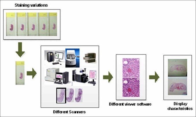
Illustration on the causes of color variations in histological images

Staining Protocol

Tissue processing and staining protocols affect the staining conditions of histological slides. Parameters, such as tissue thickness, stain concentration, and staining time have been shown to have an effect on the resultant staining color of the sectioned tissue.[13,14,15] For example, the staining color intensities of thicker tissue sections are stronger compared with thinner tissue sections.

Whole Slide Scanning

There are now a number of whole slide scanners available in the market which could digitize histological slides at high resolutions.[16,17] The production of digital slides involves a series of steps wherein specifications of the optical and hardware components of the scanner as well as the software design for the color image reproduction of the histological slides play critical roles. Since whole slide scanner makers don’t share common standards for the color reproduction software nor for the specifications of the scanner's components color variations exist in the digital slides produced by whole slide scanners of different makers.

Display

Displays are an integral part of a digital pathology system. Instead of examining stained histological slides under a microscope we view their digital images on computer displays. It is pointed out in[18] that the displays’ characteristics, i.e., luminance, contrast, resolution, color primaries, color gamut and white point, could have an effect on the color presentation of medical images. Various protocols to calibrate displays have been proposed in literatures.[19,20,21] The authors in[18] particularly re-introduced the calibration protocol in[19] to investigate the impact of calibrated displays on pathology diagnosis. Although the results of their study did not show significant difference in the diagnostic interpretations of pathologists on histopathology images shown on either un-calibrated or calibrated color displays, the results showed that pathologists rendered their interpretations faster with properly calibrated displays.

Image Viewer

With the rising popularity of whole slide imaging it is now possible for user to view whole slide images with different viewer software. Whole slide image viewers are generally developed by vendors of whole slide scanners. The color reproduction parameters of an image viewer are therefore tuned to the characteristics of the vendor's own whole slide scanner. It could then be possible to observe color variations in the original colors of the scanned images when they are viewed with an image viewer which was not originally designed for them. Integration of color enhancement in the image viewer color reproduction pipeline could also be another cause for color variations. To this date, there is no consensus yet for a standard image format for whole slide images. The way how different viewer software handles the color information embedded in the proprietary whole slide image formats could also cause the color of the displayed images to vary from their original scanned colors.

When assessing whether the colors of the digital slides (or whole slide images) reflect the colors of their physically stained slides, it is ideal that we have the physical slides. However, in the realm of digital pathology the physical slides are not necessarily available. To normalize the color variations in whole slide images produced by different whole slide scanners we introduced in this paper the use of a color calibration slide which was originally introduced in[13] to evaluate the color reproduction accuracy of display monitors. The color calibration slide is akin to that of a Macbeth color checker whose spectral colors are popularly utilized as reference in calibrating image acquisition systems[22] and displayed images.[23] The effectiveness of the color calibration slide in[13] to normalize the color variations in stained histological images was initially investigated in.[24] While there are already various methods proposed in literatures to normalize or standardize the colors of stained histological images[14,15,25,26,27,28] the use of a calibration slide for color normalization or standardization is attractive since there is no need to calculate for the pixels’ color-statistics, which could be very variable depending on the types of objects present in the image. In this work, we further investigated the utility of the color calibration slide introduced in[13] in normalizing the color variations in the scanned images of H & E stained histological slides. The results of the color correction were evaluated in two aspects: (i) colorimetric difference between the color-corrected images of the same histological slide scanned with different whole slide scanners; and (ii) color analysis on the different tissue components.

MATERIALS AND METHODS

Color Calibration Slide

The color-calibration slide for use in the color correction procedure was made in-house. The calibration slide is made with a typical glass slide embedded with nine color patches. The color patches are made from polycarbonate plastic and deep dyed polyester and create colors by allowing only to pass specific wavelengths.[29] For instance the red color patch absorbs the green and blue wavelengths and allows only the red wavelengths to pass. The mechanism by which these color patches interact with light to achieve their colors is essentially similar to the way how stained tissue sections exude their unique colors. Stained tissue sections also absorb light of certain spectral wavelengths and pass the spectral wavelengths associated to their staining. Figure 2 provides the image of the color calibration slide wherein color patches of sizes around 4 mm² are arranged at the center of the glass slide. The patches’ colors include basic colors, such as yellow, red, blue and green, and colors, which are generally observed from H & E stained tissue sections.[24] These colors were initially selected because their spectral colors span the visible spectrum, i.e., 380-720 nm. Noting that whole slide scanners were made to image stained tissue sections on glass slides we anticipate that there will be no issue scanning the color calibration slide.

Figure 2.

Color calibration slide with nine color patches

Color Spaces

Figure 3 shows the relation between color spaces. In the present color correction implementation we used the viewer software of the scanner to export the scanned images of the color patches and thereafter extract their colors. Since the viewer software outputs gamma corrected RGB (sRGB) images for display on computer monitors, inverse gamma correction was applied to the exported images to derive their linear RGB-color values, which have a linear relationship with the CIE XYZ tri-stimulus color components. The CIE XYZ color space is an additive color space, which implies that a color can be defined by adding two or three color primaries. The color spacing in the XYZ color space is not perceptually uniform. In contrast, the CIELAB color space is a perceptually uniform color space making it the choice for quantifying the perceptual color difference between images.[22] The perceptual color difference between two images can be determined by calculating the total color difference between the individual CIELAB color values of their pixels. Images are considered perceptually similar when their calculated CIELAB color difference is <2.2 units.[30]

Figure 3.

Relation between color spaces

Color Correction Procedure

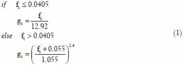
In[24] color correction is performed in the CIE XYZ color space, which means that to visualize the corrected images color space transformation, i.e., XYZ to RGB, is required. Instead of adopting this approach we adopted the approach proposed in[23] wherein color correction is implemented in the linear RGB color space rather than in the CIE XYZ color space. This could be advantageous with respect to computational cost considering the huge file size of the whole slide image. The process flow of the present color correction is illustrated in Figure 4a. First the non-linear RGB colors (or gamma corrected RGB) are converted to their linear RGB equivalents using Eq. 1.[31] The variables f_i and g_i {f_i, g_i}∈[0,1], in the equation respectively refer to the pixels’ gamma corrected RGB (or non-linear RGB) colors and their corresponding linear RGB color values at the i-th color channel, i = R, G and B

Figure 4.

(a) Color-correction scheme process flow; (b) illustration on the derivation of the color-calibration matrix for use in the color correction

Let M represent the color correction matrix. Linear combination of the coefficients of this matrix and the linear RGB color vector of a pixel, g, results to a new set of 3 × 1 color vector, g_n whose resultant color is, presumably, perceptually similar to the target color of the pixel. The linear process through which g_n is derived can be expressed in the following form:

g_n =Mg      (2)

Gamma correction is applied to the results of Eq. 2 to effectively visualize the color corrected image on ordinary color display.

The core of the present color correction method is the derivation of the color correction matrix, M, which is unique to every scanner. Figure 4b shows a basic diagram on how the color correction matrix is determined. The calculation of the matrix M requires two color data sets: The target and the scanned colors of the color patches. We will discuss in the next sections how these data sets are collected and the method by which the color calibration matrix, M, is determined.

Color Data of the Color-Patches

Target colors of the color patches

The target colors of the color-calibration patches are determined from their representative spectral transmittance samples. Let t represents the N × 1, N = 63, spectral transmittance vector of a color-patch's pixel. If F is the 3 × N matrix of the CIE XYZ color matching function, E the N × N diagonal matrix whose elements correspond to the illumination spectrum, we can calculate the 3 × 1 XYZ tristimulus vector, z, of the pixel's spectral transmittance, t as follows:[32]

z=FEt      (3)

The linear RGB color vector of the spectral transmittance t can be determined by multiplying the results of Eq. 3 with the coefficients of the 3 × 3 XYZ to RGB conversion matrix, C:

g_t = Cz,      (4)

Scanned colors of the color patches

The scanned colors of the color patches are determined from the average RGB colors of their pixels. To identify the pixels that belong to the color patches, color-based segmentation followed by pixel classification is performed on the scanned image of the color-calibration slide. The color-based segmentation is implemented using the color saturation and value, in the HSV (Hue, saturation, value) color space, of the pixels as features. The HSV color space is closely related to how humans perceive colors. In this color space the color information of an image is represented by the hue and saturation of its pixels and its brightness is represented by the color value of its pixels. Hue is what distinguishes a red from a green color, whereas saturation is associated to the amount of gray (0-100%) present in the color, i.e. a measure of the purity of a color.[33,34] To segment the color patches from the scanned image of the color calibration slide a threshold is imposed to the difference between the color saturation and value of the image pixels.[8] Pixels are labeled as color-patch pixels and assigned a value of 1 when the difference between their color saturation and value is above the set threshold otherwise they are labeled as background pixels and assigned a value of 0. To ensure that the segmented color-patches do not include some background pixels, morphological filtering is applied to the segmentation result.[35,36] Classification of the detected color patch pixels into nine classes is implemented using a mean classifier[37] with the RGB colors of the pixels as classification features. Pixel classification results to a classification map in which 0 is assigned to background pixels and numeric values 1-9 are assigned to the color-patch pixels depending on their class. To reinforce the accuracy of the classification results, majority filter was applied to the classification map wherein the class of the center pixel within an m × m, m = 3, window is assigned to the class of the majority.

Color Correction Matrix

The color correction matrix, M, is derived using the target and scanned colors of the color patches. Let G_r and G_s be 3 × 10 matrices which respectively contain the target and scanned linear RGB colors of the nine color patches, and the maximum possible grey-level values of a white area. The 3 × 3 color correction matrix M is determined using least square method as follows:

M=G_tG_s⁺      (5)

The coefficients of M will map the original color of the image pixels to their target colors. Moreover, the notation G_s⁺ denotes the Penrose pseudoinverse of the matrix G_s.

Color Analysis

The uncorrected and color-corrected scanned H & E stained images are compared and analyzed based on their CIELAB color difference values. The CIELAB color values of the image pixels can be determined in two steps. First, the linear RGB color values of a pixel are mapped into the CIE XYZ color space using Eq. 6. The results of Eq. 6 are then used in Eqs. 7 and 8 to determine the corresponding CIELAB color values of the pixel[38] The variables R, G, and B in Eq. 6 correspond to the linear RGB color values of a pixel and the variables X₀, Y₀ and Z₀, in Eq. 7 correspond to the tri-stimulus values of reference white point which, in our experiments, correspond to white point of the D65 light source.

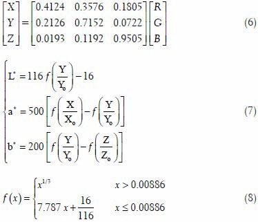
The perceptual color difference between two image pixels is proportional to the Euclidian distance between their respective CIELAB color components. The color components in the CIELAB color space are the L*, a*, and b* where L* is correlated with brightness, a* with redness-greenness and b*, with yellowness-blueness.[33] The color difference, dE^*_ab; between two pixels whose respective L*a*b* values are (L^*₁, a^*₁, b^*₁) and (L^*₂, a^*₂, b^*₂) can be computed using the expression in Eq. 9.

EXPERIMENTS AND RESULTS

Whole Slide Scanners

We used two different whole slide scanners, which we labeled as scanner A and scanner B, to scan a set of H & E stained histological slides. Both scanners feature full automatic scanning mode in which no intervention from the user is required to detect the tissue areas or identify the spatial locations of the best focus points. Although scanner A can scan a glass slide at 0.46 μ/pixel or 0.23 μ/pixel resolution its default scan-resolution is at 0.46 μ/pixel. Moreover, scanner B scans a slide at a default resolution of 0.25 μ/pixel. Furthermore, both scanners have their own viewer software which allows us to view and navigate the digital versions of the histological slides at different magnifications. It was noted that the color of the patches do not significantly vary at different pixel resolution, i.e., 0.23 μ/pixel (40×) and 0.46 μ/pixel (20×). Images are considered to be perceptually similar in color when their CIELAB color difference, is below about 2.2 units[30] and the resultant dE^*_ab between the color patches at different pixel resolution is about 1.4 units.

Color-Patches Data

Target Color of the Color Patches

63 spectral images, i.e., N = 63 bands, of the color patches with spatial dimensions of 1344 × 1024 were captured from 410 to 720 nm at a step of 5 nm using a microscopic multispectral imaging system.[39] From the multispectral image of a color patch, i.e. 63-band image, 20 spectral transmittance samples were randomly extracted. The spectral characteristics of the color patches are represented by the mean spectra of their 20 spectral samples, as shown in Figure 5a. The resultant RGB colors calculated from the patches’ transmittances will serve as the target colors of the patches’ in the implementation of the color correction. The color palettes in Figure 5b demonstrate the target colors of the patches after applying gamma correction to the results of Eq. 3.

Figure 5.

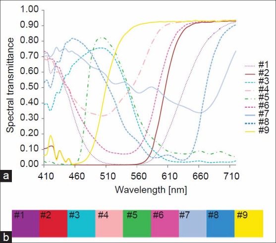
(a) Characteristics spectral transmittance of the color patches; (b) red, green, and blue color representation of the color patches transmittance spectra

Scanned Color of the Color Patches

The color patches were detected and classified from the lower resolution version (~0.5×) of the high resolution whole slide images of the color-calibration slide utilizing the procedure outlined in the color correction section in Method. The color strips at the upper panel in Figure 6 demonstrate the scanned colors of the nine color patches as reproduced by scanners A and B. The bar plots in Figure 6b, which correspond to the CIELAB color difference between the scanned colors of the patches and their target spectral colors, demonstrate the color reproduction accuracy of the scanner with respect to the given color patches. The scanned color of a color patch is closer to its target spectral color when the height of its bar is shorter. Although both scanners exhibit similar error tendencies, they differ in their accuracy level in reproducing the colors of specific patches. For example, for the blue patch, i.e. patch #7 it is scanner A that is more likely to reproduce the patch's color more accurately but for the red patch, i.e. patch #2 it is scanner B rather than scanner A.

Figure 6.

(a) Red, green, and blue colors of the color patches as reproduced by scanner A and scanner B. (b) CIELAB color difference between the scanned color of the color patches and their respective target colors

Histological Images

H & E staining is by far the most popular staining used in histopathology laboratories. The stain emphasizes the difference between cytoplasm and nuclear regions. A poll of eight randomly-selected H & E stained histological slides of different tissue types with varying staining condition and thickness (i.e., 4 or 5 μ) were considered in our experiments. The tissue types include liver, breast, lymph, intestine and brain. The slides were scanned with scanner A and scanner B, at their default resolutions, i.e., scanner A at 0.46 μ/pixel and scanner B at 0.25 μ/pixel.

Color Correction

Figure 7 displays the thumbnail images of the H & E stained whole slide images of lymph and liver tissues. The uncorrected images are displayed at the top panel and the color-corrected images are displayed at the lower panel. Whereas color variations are evident between the uncorrected images of scanner A and scanner B, such color variations are not directly observed from the color-corrected images at the lower panel implying that color variations among histological images can be normalized by applying the present color correction scheme. Details of the color analysis between the H & E stained scanned images will be presented in the next section.

Figure 7.

Thumbnail images of the high resolution whole slide images of liver and lymph tissues. Images at the first rows correspond to liver tissue while those at the second rows correspond to lymph tissue. The uncorrected images at the top panel demonstrate the existence of color variations between images produced by the two scanners. The corrected images at the lower panel illustrate the effectiveness of the present color correction scheme to normalize the color variations

Color Analysis

H & E stained images

Using the respective viewer software of the whole slide scanners A and B, we randomly identified 10 regions from each of the H & E stained whole slide images scanned at the default resolution of the scanners. Representative images of these regions were exported in Jpeg image format using the image-export functions of the viewers. The exported images of scanner A and B have different spatial dimensions, 1280 × 960 pixels for scanner A and 1268 × 608 pixels for scanner B and different pixel resolutions. To evaluate the perceptual color difference between two images in pixel-wise manner it is important that the images mirror each other, i.e. contain the same objects in the same orientations and spatial locations. Template matching algorithm, as implemented in Open Source Computer Vision,[35,36] was utilized to find for identical regions from the already re-sampled images of scanner B using the 400 × 400 pixel images which were manually cropped from 1280 × 960 images of scanner A. A total of 320, 400 × 400 pixel images were collected from this process, i.e., eight histological slides × 10 representative images × 2 regions of interest × 2 scanners. The CIELAB color differences, dE^*_ab, between the 400 × 400 pixel images of scanner A and scanner B were calculated and the results are presented in Table 1. These results demonstrate the effectiveness of the color calibration slide to normalize color variations between histological images produced by different whole slide scanners. For instance, the average color difference between the breast images scanned with scanner A and that of scanner B before correction is 5.34, but this has been considerably reduced to 1.37 after application of the color correction. The significance of these results was further validated by the results of an independent t-test statistical analysis. The analysis showed that the reduction in the average color difference between scanned images A and B after color correction, ( = 2.31, p < 0.001) was significant at 95% confidence level.

Table 1.

Average color difference, between the 400×400 pixel images of scanner A and scanner B

Figure 8 displays representatives of the 320 400 × 400 pixel images which were used to derive the results presented in Table 1. Images before and after correction are respectively arranged at the left and right panels. Moreover, the images of scanner A are arranged in columns A and those of scanner B are arranged in columns B. While the color difference between the original images of scanner A and B is obvious, this difference is minimized after the application of present color correction scheme. These images provide us visualization on the effectiveness of the present color correction scheme to normalize color differences between images produced by different whole slide scanners.

Figure 8.

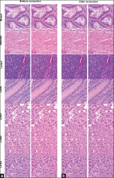
400 × 400 pixels high resolution (×20) images extracted from the whole slide images of the different histological slides. The left and right panels show the uncorrected and corrected images of scanner A and scanner B, respectively

Tissue components

In most automated histopathology image analysis the colors of the tissue components are used as main features.[25,27] Digital image analysis algorithms require some parameters to be set to optimize the analysis results. Apparently, the parameter settings optimized for images produced by one whole slide scanner may not necessarily apply for images produced by another scanner. We investigated the effect of color correction on specific tissue components such as the nuclei, cytoplasm and red blood cells (RBC). For this experiment we considered the three histological slides of liver tissue. We extracted at least 4000 color samples for each of the different tissue components from the 400 × 400 pixel images. Figure 9 shows the cluster plots of these tissue components in the chromatic plane, along a *−b* axes, of the CIELAB color space. The color clusters of the tissue components are labeled “A” and “B” to denote their source images, i.e., scanner A or scanner B images. An overlap between cluster A and cluster B implies that the colorimetric characteristics of the tissue component being compared are similar in both source images. We note that after application of color correction the clusters from different source images, i.e. scanner A and B images, overlap for the most part demonstrating that the present color correction was effective in normalizing the color differences in the tissue components. The histogram of the b* color components of nuclei and cytoplasm tissue components shown in Figure 10 further illustrate the effect of the present color correction in normalizing existing color differences. The results of an independent paired t-test analysis revealed that the average mean reduction in the color difference (μ_Nu = 5.32, μ_Cyto = 4.52, μ_RBC = 0.004) was significantly greater than 0 (P_Nu < 0.001, P_Cyto < 0.001, P_RBC < 0.004) at 95% confidence level.

Figure 9.

Cluster plots of the different tissue components projected onto the a-b chromaticity axes of the CIELAB color space. An overlap between A and B clusters implies that the color of the tissue components in scanned images A and B are similar

Figure 10.

Histograms of the CIELAB b* color values for Nuclei and cytoplasm. Each histogram was constructed using 5400 color samples. The scanner used to capture the images from which the tissue component samples were extracted is identified by the letter appended to the tissue component's name, i.e., A or B; (a) before correction; (b) after correction

DISCUSSION

Whole slide imaging technology clearly has its benefits in pathology practice. However, there are still issues that needed to be resolved before it can be fully integrated to pathology diagnosis work flow. Color standardization of histological images is one of the impending issues in digital pathology.[13] In this paper, we proposed a method to normalize the color variations in images produced by different whole slide scanners. The color correction paradigm we proposed does not only provide consistent color visualization of the histological images, but it also preserves the color fidelity of the different tissue components, i.e. no color artifacts. The color correction method is also fully integrable to whole slide scanning process and could be easily added as feature to whole slide viewer software by keeping the color correction matrix as well as the target colors of the color-calibration patches. Furthermore, the proposed color correction does not rely on the color statistics of the image pixels. In effect, color artifacts, which specially appear in the corrected image when different types of objects are found in target and test images do not necessarily appear in the corrected images.

Color-Correction Implementation

There are two ways by which color standardization using the color calibration slide can be implemented: (i) During scanning of the histological slides; or (ii) after scanning. In both cases the data entries of the color calibration matrix, Eq. 5, are needed. This implies that the target colors of the color calibration patches have to be saved in an accessible drive directory, and the color calibration slide should be scanned first to determine the scanned colors of the patches. With the color correction matrix at hand, color correction can proceed as desired, either during the scanning or after the scanning. When color correction is implemented during slide scanning the target spectral colors of the color-calibration patches can be incorporated into the color profile of the scanner. On the other hand, when color correction is desired to be implemented after scanning the histological slide, a special function could be integrated to the viewer software to allow users to interactively invoke the color correction procedure to correct the colors of the whole slide images. Although we implemented the color correction in the linear RGB space the present correction paradigm can also be implemented in the CIE XYZ or CIELAB color space.

Image Analysis Application

Digital image analysis algorithms designed for H & E stained images generally address the segmentation of nuclei, specifically the delineation between the cytoplasm and nuclei areas. The general approach to segment nuclei from H & E stained images is to employ a threshold on the color values of the pixels wherein the appropriate threshold value is determined from the color histograms of training images. This approach, however, will only yield good result when the training and test images exhibit similar colorimetric characteristics otherwise the result will be unpredictable. Nuclei are stained blue to purple by hematoxylin dye while cytoplasm and the connective tissues are stained pink to red by the eosin dye. The histograms of the b* color values, which express the pixels’ blueness, of the nuclei and cytoplasm shown in Figure 10 demonstrate that robust image analysis can be achieved with the integration of color correction process to the analysis pipeline. Application of color correction will allow identification of threshold value that works for different sets of images without regard of their colorimetric variations. Particularly, the histograms presented in Figure 10a illustrate that it is difficult to identify a threshold value which perfectly works for different sets of images, especially when the given sets of images have differing colorimetric characteristics. On the contrary, the histograms in Figure 10b show that by employing the present color correction, it could be possible to utilize the same threshold to segment the nuclei from different sets of images. These results are indicative of the need for color standardization to achieve consistency in histological image analysis results.

Limitations

The present color correction scheme is not without limitations. The heights of the bar plots in Figure 11 correspond to the average color difference of the same tissue components found in scanned images A and B. It can be concluded from this plot that with the current color correction set-up it is a challenge to correct the color of the RBC. In[40] the authors argued that it is not sufficient to use the dye amount information of the stained tissue images to correct the color of the RBC. This mainly implies that correcting the color of RBC requires a more sophisticated color correction approach than what we are currently proposing. However, since the main concern when we observe and analyze H & E stained images is the contrast between the nuclei and the cytoplasm regions this particular issue can be practically ignored.

Figure 11.

CIELAB color difference of the different tissue components between scanner A and scanner B images. The colors of the tissue component found in scanner A and scanner B images are closer when the heights of their bar plots are shorter

Figure 1 illustrates to us the possible factors behind the color variations in digital slides. The method we present in this paper addresses the color variations due to utilizing different whole slide scanning systems. When the observed color variations are caused by variability in the tissue's staining conditions, and others, the present method may not effectively work.

CONCLUSIONS

There is a continued discussion on color standardization in whole slide images. We have mentioned four possible causes for the color variations in histological images. In this paper, we particularly focused on addressing the color variations caused by the different characteristics, both in hardware and software designs, of whole slide scanners by proposing the use of a color calibration slide. The color correction method presented in this paper can easily be integrated to the slide scanning process or added as feature to the whole slide viewer software. The method is also handy in the sense that the data needed for color correction are extracted from the color calibration slide wherein the number of color patches embedded on the glass slide and the spectral colors of these patches are known beforehand. The different color patches in the current color calibration slide were originally selected to correct H & E stained images.[13] The color specifications of the color patches and their count can also be modified to accommodate other types of staining. Moreover, although the effectiveness of the present color correction method has been demonstrated, especially on H & E stained images, it still remains to be investigated whether this has a profound impact on the accuracy of pathology diagnosis. An observer study would be the ultimate test in this respect.

REFERENCES

- 1.Al-Janabi S, Huisman A, Willems SM, Van Diest PJ. Digital slide images for primary diagnostics in breast pathology: A feasibility study. Hum Pathol. 2012;43:2318–25. doi: 10.1016/j.humpath.2012.03.027. [DOI] [PubMed] [Google Scholar]
- 2.Rocha R, Vassallo J, Soares F, Miller K, Gobbi H. Digital slides: Present status of a tool for consultation, teaching, and quality control in pathology. Pathol Res Pract. 2009;205:735–41. doi: 10.1016/j.prp.2009.05.004. [DOI] [PubMed] [Google Scholar]
- 3.Wilbur DC, Madi K, Colvin RB, Duncan LM, Faquin WC, Ferry JA, et al. Whole-slide imaging digital pathology as a platform for teleconsultation: A pilot study using paired subspecialist correlations. Arch Pathol Lab Med. 2009;133:1949–53. doi: 10.1043/1543-2165-133.12.1949. [DOI] [PMC free article] [PubMed] [Google Scholar]
- 4.Stathonikos N, Veta M, Huisman A, van Diest PJ. Going fully digital: Perspective of a Dutch academic pathology lab. J Pathol Inform. 2013;4:15. doi: 10.4103/2153-3539.114206. [DOI] [PMC free article] [PubMed] [Google Scholar]
- 5.Graham AR, Bhattacharyya AK, Scott KM, Lian F, Grasso LL, Richter LC, et al. Virtual slide telepathology for an academic teaching hospital surgical pathology quality assurance program. Hum Pathol. 2009;40:1129–36. doi: 10.1016/j.humpath.2009.04.008. [DOI] [PubMed] [Google Scholar]
- 6.McClintock DS, Lee RE, Gilbertson JR. Using computerized workflow simulations to assess the feasibility of whole slide imaging full adoption in a high-volume histology laboratory. Anal Cell Pathol (Amst) 2012;35:57–64. doi: 10.3233/ACP-2011-0034. [DOI] [PMC free article] [PubMed] [Google Scholar]
- 7.Isse K, Lesniak A, Grama K, Roysam B, Minervini MI, Demetris AJ. Digital transplantation pathology: Combining whole slide imaging, multiplex staining and automated image analysis. Am J Transplant. 2012;12:27–37. doi: 10.1111/j.1600-6143.2011.03797.x. [DOI] [PMC free article] [PubMed] [Google Scholar]
- 8.Bautista PA, Yagi Y. Improving the visualization and detection of tissue folds in whole slide images through color enhancement. J Pathol Inform. 2010;1:25. doi: 10.4103/2153-3539.73320. [DOI] [PMC free article] [PubMed] [Google Scholar]
- 9.Hashimoto N, Bautista PA, Yamaguchi M, Ohyama N, Yagi Y. Referenceless image quality evaluation for whole slide imaging. J Pathol Inform. 2012;3:9. doi: 10.4103/2153-3539.93891. [DOI] [PMC free article] [PubMed] [Google Scholar]
- 10.Xiong W, Tian Q, Lim J. Proceedings of the 3rd IEEE Industrial and Electronics Applications Conference; 2008. An adaptive enhanced focusing technique for whole slide imaging using contextual information; pp. 1837–40. [Google Scholar]
- 11.Geusebroek JM, Cornelissen F, Smeulders AW, Geerts H. Robust autofocusing in microscopy. Cytometry. 2000;39:1–9. [PubMed] [Google Scholar]
- 12.Yagi Y, Gilbertson JR. A relationship between slide quality and image quality in whole slide imaging (WSI) Diagn Pathol. 2008;3(Suppl 1):S12. doi: 10.1186/1746-1596-3-S1-S12. [DOI] [PMC free article] [PubMed] [Google Scholar]
- 13.Yagi Y. Color standardization and optimization in whole slide imaging. Diagn Pathol. 2011;6(Suppl 1):S15. doi: 10.1186/1746-1596-6-S1-S15. [DOI] [PMC free article] [PubMed] [Google Scholar]
- 14.Magee D, Treanor D, Crellin D, Shires M, Smith K, Mohee K, et al. Proceeding of the Optical Tissue Image Analysis in Microscopy, Histopathology and Endoscopy (MICCAI Workshop); 2009. Colour normalisation in digital histopathology images; pp. 100–11. [Google Scholar]
- 15.Abe T, Murakami Y, Yamaguchi M, Ohyama N, Yagi Y. Color correction of pathological images based on dye amount quantification. Opt Rev. 2005;12:293–300. [Google Scholar]
- 16.Weinstein RS, Descour MR, Liang C, Barker G, Scott KM, Richter L, et al. An array microscope for ultrarapid virtual slide processing and telepathology. Design, fabrication, and validation study. Hum Pathol. 2004;35:1303–14. doi: 10.1016/j.humpath.2004.09.002. [DOI] [PubMed] [Google Scholar]
- 17.Rojo MG, García GB, Mateos CP, García JG, Vicente MC. Critical comparison of 31 commercially available digital slide systems in pathology. Int J Surg Pathol. 2006;14:285–305. doi: 10.1177/1066896906292274. [DOI] [PubMed] [Google Scholar]
- 18.Krupinski EA, Silverstein LD, Hashmi SF, Graham AR, Weinstein RS, Roehrig H. Observer performance using virtual pathology slides: Impact of LCD color reproduction accuracy. J Digit Imaging. 2012;25:738–43. doi: 10.1007/s10278-012-9479-1. [DOI] [PMC free article] [PubMed] [Google Scholar]
- 19.Silverstein LD, Hashimi SF, Lang K, Krupinski EA. Paradigm for achieving color reproduction accuracy in LCDs for medical imaging. J Soc Inf Disp. 2012;20:53–62. [Google Scholar]
- 20.Rodriguez-Pardo CE, Sharma G, Feng XF. Proceedings ICASSP; 2013. Two dimensional color calibration for four primary displays; pp. 2820–4. [Google Scholar]
- 21.Proceedings the 1st International Conference on Bioinformatics and Bioengineering; 2007. DICOM GSDF based calibration method of general LCD monitor for medical softcopy image display; pp. 1153–6. [Google Scholar]
- 22.Vander Haeghen Y, Naeyaert JM, Lemahieu I, Philips W. An imaging system with calibrated color image acquisition for use in dermatology. IEEE Trans Med Imaging. 2000;19:722–30. doi: 10.1109/42.875195. [DOI] [PubMed] [Google Scholar]
- 23.Van Poucke S, Haeghen YV, Vissers K, Meert T, Jorens P. Automatic colorimetric calibration of human wounds. BMC Med Imaging. 2010;10:7. doi: 10.1186/1471-2342-10-7. [DOI] [PMC free article] [PubMed] [Google Scholar]
- 24.Murakami Y, Gunji H, Kimura F, Yamaguchi M, Yamashita S, Saito Akira, et al. Conference Proceeding 20th Color Imaging Conference; 2012. Color correction in whole slide digital pathology; pp. 253–8. [Google Scholar]
- 25.Kothari S, Phan JH, Moffitt RA, Stokes TH, Hassberger SE, Chaudry Q, et al. Conference Proceeding ISBI; 2011. Automatic batch-invariant color segmentation of histological cancer images; pp. 657–60. [DOI] [PMC free article] [PubMed] [Google Scholar]
- 26.Macenko M, Niethammer M, Marron JS, Borland D, Woosley JT, Xiaojun G, et al. Conference Proceeding ISBI; 2009. A method for normlaizing histology slides for quantitative analysis; pp. 1107–10. [Google Scholar]
- 27.Monaco J, Hipp J, Lucas D, Smith S, Balis U, Madabhushi A. Image segmentation with implicit color standardization using spatially constrained expectation maximization: Detection of nuclei. Med Image Comput Comput Assist Interv. 2012;15:365–72. doi: 10.1007/978-3-642-33415-3_45. [DOI] [PubMed] [Google Scholar]
- 28.Mosquera-Lopez C, Agaian S. Proceeding SPIE 8755, Mobile/Image Processing, Security, and Applications; 2013. Iterative local normalization using fuzzy image clustering. 875518. [Google Scholar]
- 29. [Last accessed 2013 Nov 24]. Available from: http://www.rosco.com/filters/roscolux.cfm .
- 30.Stokes M, Fairchild MD, Berns RS. Precision requirements for digital color reproduction. ACM Trans Graph. 1992;11:406–22. [Google Scholar]
- 31.Valous NA, Mendoza F, Sun DW, Allen P. Colour calibration of a laboratory computer vision system for quality evaluation of pre-sliced hams. Meat Sci. 2009;81:132–41. doi: 10.1016/j.meatsci.2008.07.009. [DOI] [PubMed] [Google Scholar]
- 32.Shinoda K, Murakami Y, Yamaguchi M, Ohyama N. Lossless and lossy coding for multispectral image based on sRGB standards and residual components. J Electron Imaging. 2011;20:023003. [Google Scholar]
- 33.Pratt WK. 4th ed. New Jersey, USA: A John Wiley and Sons, Inc. Publication; 2007. Digital Image Processing; p. 46. [Google Scholar]
- 34.Cheng HD, Jiang XH, Sun Y, Wang J. Color image segmentation: Advances and prospect. Pattern Recognit. 2001;34:2259–81. [Google Scholar]
- 35.Bradski G, Kaehler A. Sebastopol, CA, USA: O’Reilly Media, Inc; 2008. Learning Open CV Computer Vision with the Open CV Library? p. 115. [Google Scholar]
- 36. [Last accessed on 2013, November 24]. Available from: http://www.opencv.org/downloads.html .
- 37.Duda RO, Hart PE, Stork DG. 2nd ed. New York, New York, USA: John Wiley and Sons, Inc; 2001. Pattern Classification; p. 182. [Google Scholar]
- 38.Wang X, Zhang D. An optimized tongue image color correction scheme. IEEE Trans Inf Technol Biomed. 2010;14:1355–64. doi: 10.1109/TITB.2010.2076378. [DOI] [PubMed] [Google Scholar]
- 39.Bautista PA, Yagi Y. Digital simulation of staining in histopathology multispectral images: Enhancement and linear transformation of spectral transmittance. J Biomed Opt. 2012;17:056013. doi: 10.1117/1.JBO.17.5.056013. [DOI] [PubMed] [Google Scholar]
- 40.Abe T, Haneishi H, Bautista PA, Murakami Y, Yamaguchi M, Ohyama N, Yagi Y. Barcelona, Spain: Proceeding Computer Graphics, Imaging and Visualization Conference 2008; 2008. Color correction of red blood cell area in H & E stained images by using multispectral imaging; pp. 432–6. [Google Scholar]