Magnetic Resonance Image Example Based Contrast Synthesis

Abstract

The performance of image analysis algorithms applied to magnetic resonance images is strongly influenced by the pulse sequences used to acquire the images. Algorithms are typically optimized for a targeted tissue contrast obtained from a particular implementation of a pulse sequence on a specific scanner. There are many practical situations, including multi-institution trials, rapid emergency scans, and scientific use of historical data, where the images are not acquired according to an optimal protocol or the desired tissue contrast is entirely missing. This paper introduces an image restoration technique that recovers images with both the desired tissue contrast and a normalized intensity profile. This is done using patches in the acquired images and an atlas containing patches of the acquired and desired tissue contrasts. The method is an example-based approach relying on sparse reconstruction from image patches. Its performance in demonstrated using several examples, including image intensity normalization, missing tissue contrast recovery, automatic segmentation, and multimodal registration. These examples demonstrate potential practical uses and also illustrate limitations of our approach.

I. Introduction

Magnetic resonance (MR) imaging (MRI) is widely used to image the brain. Postprocessing of MR brain images, e.g., image segmentation [1]–[6] and image registration [7]–[11], has been used for many scientific purposes such as furthering our understanding of normal aging [12], [13], disease progression [14], [15], population analysis [16], and prognosis [17]. It is well known that image analysis algorithms are routinely optimized for a particular type of scan (or collection of scans), which could include specification of the tissue contrast (e.g., T1-weighted (T1-w) versus T2-weighted (T2-w)), image resolution, pulse sequence parameters, field strength of the scanner, and even the particular scanner manufacturer. Although many algorithms claim to be robust to variations in the input images, inevitably there will be performance degradation as the input images deviate from a perfect match to the images that were used to carry out the algorithm optimization.

There are many practical situations, including multi-institution trials [18]–[20], rapid emergency scans [21], and scientific use of historical data [12], where the images are not acquired according to an optimal protocol for a given image analysis algorithm. As well, a particular tissue contrast that is necessary for a given algorithm might have been omitted for a given study or for a particular patient acquisition. In such cases, investigators and clinicians have three choices. First, they might apply the algorithm on available images and accept a sub-optimal result. Second, they might remove patients with inadequate image data from the study. Third, they might design a new image analysis algorithm that will work equally well on the image data that is available to them. Upon consideration of these options, it seems that each choice leads to concerns, and an alternative is highly desirable. This paper is concerned with a fourth alternative: to recover an image with the desired tissue contrast and intensity profile using the available images and prior information. There are three general approaches described in the literature to carry out this fourth alternative, which we briefly describe next. The method we describe in this paper offers an approach with significant advantages over existing approaches including improved performance and greater applicability.

The most common approach to recovery of images with a desired tissue contrast and intensity profile is histogram matching [22]–[29]. Some manner of histogram matching is used as a preprocessing step in nearly every neuroimage segmentation and registration pipeline because they do improve the accuracy and consistency of results [30], [31]. However, its use becomes questionable when applied to data acquired with different pulse sequences, especially when pathology is present, and its use in volumetric analysis may lead to incorrect results simply because the histograms are forced to follow that of a target image which itself contains certain ratios of tissue types. One way to address this last concern is to first segment brain structures and match their individual histograms to a registered atlas [32]. Although this method produces consistent subcortical segmentations over data sets acquired under different scanners, it requires a detailed segmentation of the images before intensity normalization has been applied, which leads to a “chicken and egg” situation. It is clearly more desirable to normalize the image intensities prior to any significant image analysis algorithms have been applied.

A second approach to recover images with a desired tissue contrast and intensity profile is to acquire multiple images of the subject with predefined, precisely calibrated acquisition parameters [33]. Given this set of images, tissue proton density P_D and relaxation parameters T₁, T₂, and $T_2^{\ast }$ can be estimated by inverting the pulse sequence equations [34], and calibrated images with the desired tissue contrast can be computed by using these estimated parameters in the appropriate mathematical equation derived from the imaging physics [35]. This approach has three disadvantages. First, the imaging equations are typically only an approximation to what is used in practice, and therefore the acquired data may not be accurately related to the underlying tissue parameters by the assumed imaging equation. Second, the required voxel-wise mathematical inversion is generally poorly conditioned, which means that noise and artifacts can have a large impact on the accuracy of estimating the underlying tissue parameters. Third, in large imaging studies with many clinical scenarios it is difficult to acquire the source image data with consistent, predefined image acquisition parameters. Because of these problems, most image processing algorithms are not designed to exploit the existence of underlying tissue parameter estimates nor are most studies and clinical scans designed to exploit this approach to tissue contrast normalization.

Another way to recover a target tissue contrast and intensity profile is to register the subject to a multiple-contrast atlas and to transfer the desired contrast intensities from the atlas space to the subject space [36]. This approach enjoys great popularity not only for transferring tissue contrasts but also for transferring segmented tissue labels [37], and is tacitly assumed by many researchers to be the best current approach for generation of images with alternate tissue contrast. However, this approach does not produce an acceptable result if the registration result is poor or if there are anomalies or unknown tissues in the subject that are not present or spatially distributed differently in the atlas. In the example shown in Fig. 1, a T1-w spoiled gradient recalled (SPGR) atlas (Fig. 1(a)) was registered to a similar contrast subject image (Fig. 1(c)) using the (inverse consistent and diffeomorphic) SyN registration algorithm [7]. The atlas magnetization prepared rapid gradient echo (MPRAGE) contrast intensities (Fig. 1(b)) were then mapped through the transformation to the subject space, yielding a synthetic subject MPRAGE image (Fig. 1(e)). By comparing this result to the subject’s true MPRAGE image (Fig. 1(d)), it is apparent that this approach failed to adequately define the ventricles (Fig. 1(d), arrow adjacent to the ventricles) due to shortcomings in the registration, and it also failed to represent the WM lesions that are present in the original image (Fig. 1(d), arrow denoting the lesion posterior to the ventricles) because such lesions are not present in the atlas. The image produced using our approach (Fig. 1(f)) shows neither of these problems and compares quite favorably in overall contrast and appearance to the true MPRAGE.

Fig. 1.

(a) Atlas T1-weighted SPGR and (b) its corresponding T1-weighted MPRAGE. (c) A subject T1-weighted SPGR scan and (d) its T1-weighted MPRAGE image. The atlas SPGR is deformably registered (using SyN [7]) to the subject SPGR. This deformation is applied to the atlas MPRAGE to obtain (e) a synthetic subject MPRAGE. (f) The synthetic MPRAGE image generated by our algorithm, MIMECS.

The method proposed in this paper, MR image example-based contrast synthesis (MIMECS), combines the idea of example-based image hallucination [38], [39] with non-local means [40]–[42] and sparse priors [43], [44] to synthesize MR contrasts using patches—i.e., small regions of the image—from a multiple-contrast atlas (also called a textbook in [36]). The core idea of MIMECS is that each subject patch can be matched to a combination of a few relevant patches from a dictionary in a non-local fashion [43], [45], [46]. It is different from classical histogram matching in the sense that a patch can be thought of as a feature vector of its center voxel, thus including local neighborhood information for that voxel. We show the results of seven case studies which demonstrate potential uses and limitations of MIMECS in realistic scientific and clinical scenarios.

There are several advantages of MIMECS compared to previous synthesis methods. First, it is a completely automatic pre-processing step that can precede any image processing task. Second, there is no need to use multiple, calibrated pulse sequences in order to estimate underlying tissue parameters. Third, even though MIMECS uses an atlas, there is no need to carry out subject-to-atlas registration, thus avoiding potential errors due to misregistration or missing tissues. Finally, it does not require any segmentation of the subject. This last point, detailed in Sec. III-C, is a unique feature of this work improving on our previous patch based results [47]–[49], and is important in the field of sparse reconstruction as it alleviates the need for atlas training.

The paper is organized as follows. First, we summarize the idea of sparse priors and establish some notation that will be used throughout the paper. Then the atlas based patch matching synthesis algorithm is explained in a sparse priors paradigm, Fig. 2 provides a high level overview of the algorithm. Finally, we demonstrate the applicability of MIMECS on a variety of case studies.

Fig. 2.

An illustration of the MIMECS algorithm. The region of the image labeled A, shows the construction of the atlases A₁ and A₂, see Section III-A for details. Region B shows the input subject images converted into patches b₁(j). Region C denotes the estimation of the coefficients x(j) which relate b₁(j) to the patches of the atlas A₁. Finally, region D shows the computation of the synthetic image ŝ_n+1 by using the learned coefficients x(j) to compute the patch b̂₂(j) based on the atlas A₂. Section III-B describes regions B, C, and D.

II. Background

Sparse signal reconstruction maintains that because most signals are sparse in some way it is not necessary to observe the full signal in order to accurately reconstruct it. The idea has been successfully applied to many image processing algorithms including denoising [46], image restoration [50], [51], and super-resolution [43], often improving on state-of-the-art algorithms. For example in [46], authors use a K-SVD algorithm [52] to generate an overcomplete set of bases from natural image patches and apply it to a denoising problem. Dictionary based patch matching methods [53], [54] are also popular for natural image restoration. In our case, we build an overcomplete dictionary using patches from human brain images to both normalize a given contrast and synthesize alternate MR tissue contrasts. This section presents the mathematical formulation and key results that are needed to explain our approach.

Suppose we want to reconstruct a vector x ∈ ℝ^N that is s-sparse, i.e., having at most s non-zero elements, and our observations are b = Ax, where b ∈ ℝ^d, s < d < N, and A ∈ ℝ^d×N. Since this is an under-determined system, we cannot directly invert the system to find x, and additional penalties or constraints must therefore be used. Since x is known to be sparse, it makes sense to formulate an objective function that tries to find a sparse solution that is also consistent with the measurements, as follows,

$$\widehat{\mathbf{x}}=min{\Vert \mathbf{x}\Vert }_0\text{such}\text{that}{\Vert \mathbf{b}-A\mathbf{x}\Vert }_2^2<{\epsilon }_1.$$ (1)

Here, ε₁ is the noise level in the measurements, || · ||_p is the ℓ_p norm; in particular, ||x||₀ is the number of non-zero elements in x. There are relatively simple conditions on A that guarantee a feasible solution to (1), however the solution of this problem is combinatorial in nature, and therefore NP-hard.

It has been shown that if ||x||₀ is small [55], the optimal solution to (1) can also be found by solving,

$$\widehat{\mathbf{x}}=min{\Vert \mathbf{x}\Vert }_1\text{such}\text{that}{\Vert \mathbf{b}-A\mathbf{x}\Vert }_2^2<{\epsilon }_2,$$

This is a convex programming problem and can be solved in polynomial time. If ε₂ is unknown, we can rewrite the above in the following form,

$$\widehat{\mathbf{x}}=\underset{\mathbf{x}}{argmin}\{{\Vert \mathbf{b}-A\mathbf{x}\Vert }_2^2+\lambda {\Vert \mathbf{x}\Vert }_1\},$$ (2)

where λ is a weighting factor. The resulting sparsity in x̂ decreases as λ increases. The formulation in (2) is now the standard way to frame a “sparse prior” estimation problem and is the core idea behind MIMECS.

III. Method

The MIMECS method is based on analysis of image patches, which are p × q × r 3D subimages associated with each voxel of the image. Patches are typically small and centered on the voxel of interest—e.g., p = q = r = 3 or p = q = r = 5. For convenience we write a patch as the 1D vector b of size d × 1, where d = pqr. The voxels within a patch are always ordered in the same way, using a consistent rasterization, in order to create this 1D representation. Fig. 2 provides an illustrative overview of the MIMECS algorithm.

A. Atlas description

We define an atlas as an (n + 1)-tuple of images, {a₁, a₂, …, a_n, a_n+1}, where a_k has tissue contrast , k = 1, …, n+1. All atlas images a_k are co-registered and sampled on the same voxel locations in space. At each voxel, 3D patches can be defined on each image and are denoted by the d × 1 vectors a_k(i), where i = 1, …, N, is an index over the voxels of a_k. Since a_k’s are co-registered, each of them has the exact same number of voxels N. The primary aim of MIMECS is to synthesize the contrast image using a set of n subject images having contrasts to . We define the contrast dictionary A₁, A₁ ∈ ℝ^nd×N, where the i^th column of A₁ is f(i) = [a₁(i)^T … a_n(i)^T]^T, i.e., an ordered (according to their contrasts through ) column vector composed of patches a_k(i), which is the i^th patch from the atlas a_k. The contrast dictionary A₂, A₂ ∈ ℝ^d×N, is constructed in a similar manner but only contains the patches found in the atlas a_n+1, which correspond to the tissue contrast. By construction, the i^th columns of A₁ and A₂ correspond to the same spatial location and represent the through and contrasts, respectively.

B. Contrast synthesis algorithm

We assume that there are n subject (input) images {s₁, …, s_n} available with contrasts to . They are co-registered and sampled on the same voxel locations in space. We note that {s₁, …, s_n} are not registered to {a₁, …, a_n+1}. Also, if there are fewer subject images than the number of images in the atlas, then the atlas contrasts that do not match the subject contrasts are removed, n is reduced (to a minimum of n = 1), and MIMECS is carried out on the available subject images. We first decompose the subject images s_k into d × 1 patches s_k(j), where j is an index over the voxels of s_k. For every j, we stack all the patches s_k(j) in a nd × 1 vector b₁(j), in the order of their contrasts through , b₁(j) = [s₁(j)^T … s_n(j)^T]^T, b₁(j) ∈ ℝ^nd. For simplicity of terminology, we also call any nd × 1 vector a “patch”. The aim is to obtain a synthetic contrast subject image ŝ_n+1 using {s₁, …, s_n} and {a₁, …, a_n+1}.

We assume that for a subject image patch b₁(j), a small number of relevant and similar examples can always be found from a rich and overcomplete patch dictionary, A₁, which has the same contrasts (and assembled into patch vectors in the same order) as b₁(j). It is unlikely that a single patch from A₁ will perfectly match b₁(j), but it is quite likely that an optimal linear combination of a small number of patches will yield a very close approximation. The problem of finding a few patches to form the linear combination can be solved either by comparing noise characteristics, as derived in non-local means [40]–[42], or by assuming the weight vector x(j) is sparse [44], which is the approach we take here. This leads to the following generic expression for the desired solution

$${\mathbf{b}}_1(j)\approx A_1\mathbf{x}(j),\text{for}\text{some}\mathbf{x}(j)\in {ℝ}^N,{\Vert \mathbf{x}(j)\Vert }_0\ll N,\forall j,$$ (3)

where A₁ is a subset of “relevant” patches taken from the atlas images {a₁, …, a_n}. The relevant patches are chosen according to their ℓ₂ distance from the subject patch, b₁(j), as suggested in [45]. The details are given in Sec. IV. Once the sparse weight x(j) is found, the contrast subject patch estimate is found by applying the same linear combination to the corresponding contrast dictionary, A₂, i.e.,

$${\widehat{\mathbf{b}}}_2(j)=A_2\mathbf{x}(j).$$ (4)

The idea of transferring estimated coefficients from one dictionary to another, as we do here, has been explored previously in the context of super-resolution [43] and label fusion [39], [41].

It is important to consider why we seek a sparse representation. The sparsest representation x(j) is just a single column of A₁ which is approximately equal to b₁(j). In this case, the corresponding column of A₂ gives the contrast of b₁(j). However, our formulation will not yield unit sparsity in general, but instead a small number of patches from A₁ whose linear combination gives b₁(j). The motivation behind choosing a sparse x(j) to reconstruct b₁(j) is twofold. First, to reconstruct a subject patch, we want to pick those atlas patches that are close in intensity, i.e., those that are likely to be from the same tissue classes, so it would be undesirable to pick a large number of patches that might tend to mix the tissue classes. Second, if too many similar atlas patches are used to reconstruct b₁(j), then the corresponding contrast patch will be overly smooth due to the cumulative effects of small mismatches in each patch. Empirically, we have found that non-sparse x(j) tends to produce smooth images acting much like a denoising process, while highly sparse x(j) produces noisy images. In Sec. IV, an empirical way of choosing the sparsity level is described.

Since the combinatorics of (3) makes it infeasible to solve this problem directly, we use an ℓ₁ minimization strategy and reformulate the problem as,

$$\widehat{\mathbf{x}}(j)=\underset{\mathbf{x}\ge 0}{argmin}\left[{\Vert {\mathbf{b}}_1(j)-A_1\mathbf{x}\Vert }_2^2+\lambda {\Vert \mathbf{x}\Vert }_1\right],\forall j,\text{subject}\text{to}{\Vert \mathbf{f}(i)\Vert }_2^2=1,i=1,\dots ,N,$$ (5)

where f(i) denotes the i^th column of A₁, also defined in Sec. III-A. As in (2), λ is a weighting factor that encourages a sparse solution when it is large. Given this optimal combination of the patches in A₁, which best approximates the subject patch b₁(j), the contrast patch is estimated using (4). The full contrast image ŝ_n+1 is reconstructed by taking the union of all central voxels in the reconstructed patches.

There are two key differences in our solution (5) as compared to (2). The first, is the positivity constraint on the coefficients x in (5). The reason we impose this condition is to encourage the selected patches—i.e., those used in the sparse reconstruction of the subject patch—to have the same “texture” as the subject patch. For example, we do not want a boundary that is GM on the left and WM on the right to be approximated with a negative coefficient multiplying a patch having exactly the opposite orientation. The image being approximated may “look” the same, but the underlying tissues would be wrong and a patch that is synthesized would have incorrect tissues and thus have the wrong appearance. This condition is therefore designed to encourage “gray matter patches” to be used to synthesize “gray matter patches” and so on. We note that computational aspects of this positivity constraint has been previously explored in Lasso [56], and that this constrained ℓ₁ minimization procedure has been shown to be equivalent to an ℓ₀ minimization procedure (like (1) with a similar positivity constraint) if x(j) is sufficiently sparse [57].

The second difference between (5) and (2) is the requirement that the columns of A₁ (denoted by f(i), i = 1, …, N) be normalized to unity. This constraint is necessary in order to guarantee the uniqueness of the solution (by removing the scaling ambiguity), and is a common feature of patch-based techniques in computer vision and image processing [43], [45]. However, unit normalization of patches taken from the atlas MR images, removes the relationship between overall patch intensity and the patch texture, which is essential to distinguish between a “pure” GM patch and a “pure” WM patch, which can only be differentiated by their intensities and not the texture. Therefore, in Sec. III-C we propose a novel approach that normalizes patches in the (nd + 1)-dimensional space rather than the nd-dimensional space in order to preserve the desired intensity information.

C. Normalization of A₁

To guarantee a unique solution to (5), the columns of A₁ are normalized such that ${\Vert \mathbf{f}(i)\Vert }_2^2=1$, ∀i = 1, …, N. However, if scale is directly removed from an MR image patch, then a key feature in distinguishing tissue types is lost and patches used in the sparse reconstruction are less likely to be selected from the same tissue type. It is common in the sparse reconstruction literature to use prior training to learn how to select a subset of patches from which to synthesize a given subject patch. In our prior work [47]–[49] we used an atlas selection method based on image classification in order to restrict the dictionary to patches that are likely to come from appropriate tissue classes [47], [48]. We note that the present method supports this strategy since we use a subset A₁ of patches from which to select a sparse collection (see Sec. IV). However, an important goal in the present work is to eliminate both the dependency on prior training and the requirement for a classification step prior to synthesis. We have accomplished this using the “trick” of normalizing the patches (e.g., b₁(j)’s or f(i)’s) in a (nd + 1)-dimensional space rather than the nd-dimensional space, which we now describe.

All the atlas and subject patches are first globally normalized such that their maximum of their norms is unity. Define,

$$m=\underset{i,j}{max}\{{\Vert \mathbf{f}(i)\Vert }_2,{\Vert {\mathbf{b}}_1(j)\Vert }_2\}.$$

Then the patches are scaled as follows,

$$\begin{array}{c}\stackrel{\sim }{\mathbf{f}}(i)=\frac{\mathbf{f}(i)}{m},\forall i,\\ {\stackrel{\sim }{\mathbf{b}}}_1(j)=\frac{{\mathbf{b}}_1(j)}{m},\forall j.\end{array}$$

This global scaling guarantees that relative intensities are preserved and that all intensities of both subject and atlas fall in the range [0, 1]. Now, we project both the subject patch and all atlas patches to the unit sphere in ℝ^nd+1 as follows,

$$\begin{array}{l}{\mathbf{f}}^{\prime }(i)=\left[\begin{array}{c}\stackrel{\sim }{\mathbf{f}}(i)\\ \sqrt{1-{\Vert \stackrel{\sim }{\mathbf{f}}(i)\Vert }^2}\end{array}\right],\forall i,\\ {\mathbf{b}}_1^{\prime }(j)=\left[\begin{array}{c}{\stackrel{\sim }{\mathbf{b}}}_1(j)\\ \sqrt{1-{\Vert {\stackrel{\sim }{\mathbf{b}}}_1(j)\Vert }^2}\end{array}\right],\forall j.\end{array}$$

At this point, both the subject patch and the atlas patches are normalized to unity, satisfying ${\Vert {\mathbf{f}}^{\prime }(i)\Vert }_2^2=1$, ∀i, and ${\Vert {\mathbf{b}}_1^{\prime }(j)\Vert }_2^2=1$, ∀j. The normalization criterion in (5) is therefore automatically satisfied if the contrast dictionary A₁ is changed to $A_1^{\prime }\in {ℝ}^{(nd+1)\times N}$ such that the columns of $A_1^{\prime }$ are f′(i), i = 1, …, N.

Given this new normalization, we rewrite (5) as

$$\widehat{\mathbf{x}}(j)=\underset{\mathbf{x}\ge \mathbf{0}}{argmin}\left[{\Vert {\mathbf{b}}_1^{\prime }(j)-A_1^{\prime }\mathbf{x}\Vert }_2^2+\lambda {\Vert \mathbf{x}\Vert }_1\right],\forall j.$$ (6)

The solution of (6) yields a nonnegative combination of the columns of $A_1^{\prime }$ that sparsely approximates ${\mathbf{b}}_1^{\prime }(j)$. The resulting reconstructed patch matches both the pattern and intensities within the target patch. We use this solution x̂(j) ∈ ℝ^N to synthesize the contrast subject patch in ℝd. This works correctly because we maintain the association of columns in A₁, A₂ and $A_1^{\prime }$. Once b̂₂(j) is found from (4), we use only its central value in the reconstructed image ŝ_n+1.

IV. Implementation

A. Patch size and ℓ₁ Solvers

For all the experiments reported in this and subsequent sections, we used patches of dimension 3 × 3 × 3 voxels, i.e. d = 27. We used two freely available ℓ₁ solver packages, the large-scale ℓ₁-regularized least-squares (ℓ₁_ls) [58] and CVX [59], to optimize (6). From our experience, ℓ₁_ls is the faster of the two, typically having ~ 1 ms run-time per patch, while CVX on average takes ~ 10 ms. However, CVX is more robust, managing to produce reasonable results in cases where ℓ₁_ls does not converge. Thus, we use ℓ₁_ls as our ℓ₁ solver except in the following three cases:

1. the algorithm does not converge and gives null output,

2. the output x̂(j) contains a complex number,

3. experimentally we have found that for typical SPGR images, ||x̂(j)||₁ has a Laplacian distribution [60], [61] with mean 1 and small variance (~ 0.005). Thus if ||x̂(j)||₁ ≫ 1 for some j, the algorithm is assumed to converge to an undesirable solution.

For these cases, ℓ₁_ls having failed, we use CVX.

B. Dictionary Selection

A typical 256 × 256 × 199 isotropic MR image, with voxels of size 1 mm³, contains about one million non-background patches. It is computationally intractable to solve (6) with all such patches included in the dictionary $A_1^{\prime }$. Recall that for 3 × 3 × 3 patches, our dictionary $A_1^{\prime }\in {ℝ}^{28\times N}$, could potentially be a 28 × 1, 000, 000 matrix, if N is assumed to be indexing over all patches in the atlas image a₁. To avoid the computational bottleneck of large N we construct a dictionary for each patch ${\mathbf{b}}_1^{\prime }(j)$, that is of size N = 100. This is done by selecting 100 patches from the global collection of one million patches, thus drastically reducing run time. In keeping with the literature [45], we construct our patch dictionary, $A_1^{\prime }$, to consist of only those atlas patches that are close to ${\mathbf{b}}_1^{\prime }(j)$ in an ℓ₂ sense. It is also in accordance with the assumption that the atlas patches should be close to the subject patch. To achieve this in our setting, we sort the atlas patches, ${\mathbf{f}}_1^{\prime }(i)$, i = 1, 2, …, N, by their ℓ₂ distance to the current patch, ${\mathbf{b}}_1^{\prime }(j)$. The nearest 100 patches, ${\mathbf{f}}_1^{\prime }(i)$, i = 1, 2, …, 100, are then used to generate the dictionary, $A_1^{\prime }$, for the current patch, then x̂(j) is found using (6). To accelerate the search for the 100 nearest patches, we use a k-d tree [62]. We construct $A_2^{\prime }$ as the corresponding contrast patches for the collection a₂(i), i = 1, 2, …, 100. Our selection of N = 100 is based on our experience, having observed that smaller N does not always yield the best candidate patches and larger N generally shows little improvement in the reconstruction result.

To demonstrate the validity of the choice of atlas patches using such an ℓ₂ proximity criteria between them, Table I shows the fractions of major atlas tissues used to reconstruct a subject patch, averaged over all subject patches from a 256 × 256 × 199 real SPGR image, shown in Fig. 3. The classification of the center voxel of a patch is used to classify the patch. Ideally, the table should contain 1 at the diagonal entries with 0 otherwise. From the table, 78% of the atlas patches, that are used to reconstruct the subject ventricle patches are from atlas ventricle patches, while the remainder are from atlas CSF (16%) and GM (6%). However, we have observed that the non-zero fraction of atlas GM patches used to synthesize subject ventricles can be attributed to the partial volume effect at the boundary of WM and ventricles, which is reconstructed by GM patches. Similarly, the non-zero contributions of atlas CSF and WM patches (10%) to reconstruct subject GM patches can be attributed to the partial volume near CSF-GM and GM-WM boundary. On the other hand, the zero contribution of atlas WM patches to reconstruct subject CSF patches or atlas CSF patches for subject WM patches indicate that the tissues are not “interchanged” while reconstructing, which provides evidence that the (d + 1)-dimensional normalization and the coefficient positivity aspects of the algorithm, as described in Sections III-B and III-C are working as desired.

TABLE I.

Fraction of atlas patches used, averaged over all subject patches from a 256 × 256 × 199 image, from each of cerebrospinal fluid (CSF), gray matter (GM), white matter (WM), and the ventricles (VEN).

		Atlas
		CSF	VEN	GM	WM
Subject	CSF	0.71	0.15	0.14	0.00
	VEN	0.16	0.78	0.06	0.00
	GM	0.10	0.03	0.77	0.10
	WM	0.00	0.00	0.23	0.77

Fig. 3. Effect of sparsity of x(j) on the contrast.

The left most column shows a subject’s SPGR (top) and MPRAGE (bottom) acquisitions. The second, third, and fourth columns of the top row show synthetic MPRAGEs generated using another portion of the subject’s MPRAGE as the atlas. The synthetic MPRAGEs were generated using λ values of 0.05, 0.80, and 0.95, respectively. The plot shows the MPRAGE synthesis error vs. the average sparsity of all x(j)’s, averaged over all non-zero voxels. The average sparsity scale is on the top of the plot while the sparsity regularization parameter, λ, is plotted on the bottom axis.

C. Sparsity regularization coefficient

The sparsity regularization term, λ, is an important parameter in our algorithm as it is used for tuning the sparsity of the reconstruction. Through empirical experiments involving hundreds of thousands of patch reconstructions, we have found the algorithm itself to be very stable for λ ∈ [0, 0.85]; but the quality of reconstruction varies within this range. To get a quantitative sense of the synthesis, we experimentally assessed how the error in synthesis is affected by the choice of λ. Accordingly, we created an atlas pair {a₁, a₂} using patches from one part (several contiguous slices) of a subject’s SPGR ( ) and MPRAGE ( ) and then synthesized other slices of the MPRAGE image from the SPGR. Shown in Fig. 3 are three examples of reconstructed MPRAGEs using different values of λ and a graph of the root mean square error between the synthesized MIMECS MPRAGEs and the true MPRAGE. We conclude from this experiment that values of λ in the range [0.05, 0.85] are visually acceptable and produce similar error levels. However, since our original goal was to recover a solution that satisfies an ℓ₀ criterion, we choose to use a larger λ from this range because sparser solutions produced by ℓ₁ minimization are more likely to agree with the desired ℓ₀ solution [55]. We have therefore used λ = 0.80 in all of our experimental results reported below.

V. Results

In order to verify the correctness of our MIMECS software implementation, to demonstrate its most basic behavior, and to compare it to histogram matching methods, we first made extensive use of the Brainweb phantom data [63], the Kirby-21 reproducibility data [64], and the BIRN traveling subject data [18]. These results are omitted here for paper length considerations, but they can be found in [65]. The most important results from this set of experiments can be summarized as follows. First, we found that features and noise that are present in the subject s₁ image but not in the atlas a₁ image are suppressed to some degree in the reconstruction. This was true both in recovering the same tissue contrast (a kind of “sanity check”) and in recovering different tissue contrasts. This observation suggests that MIMECS can be used for noise suppression (though other methods such as non-local means might be better) and also serves as a caution that the MIMECS atlas should contain a patch dictionary that is rich enough to encompass the patches that are expected to be found in the source image. Second, the experiments confirmed that sparsity is important when reconstructing patches with significant detail because otherwise the detail will be smoothed out. Third, MIMECS is fairly robust to the specifics of the subject pulse sequence. In particular, we found that an atlas comprising both an SPGR and MPRAGE can be used to synthesize either an MPRAGE or SPGR image even if the subject image did not precisely match the SPGR or MPRAGE pulse sequence parameters of the atlas. Fourth, we found that MIMECS normalization is comparable or better than histogram matching when normalizing the same tissue contrast (e.g., T1-w from T1-w) and, of course, is far more general in that it can recover missing contrasts. Finally, we found that errors in MIMECS synthesis do not take on specific anatomical features, but instead resemble a typical noise pattern of MR images. This was true in both normalization of the same contrasts and synthesis of alternate contrasts. We note that most of the above observations will be evident in the results below, which is another reason why we did not include these results here.

In this section, we focus on potential uses of MIMECS in clinical and scientific studies rather than focusing solely on performance-oriented criteria (since we have previously reported such results in [47]–[49], [65]). Accordingly, each result should be thought of as a “case study” designed to demonstrate a potential use. Some studies provide numerical results that demonstrate improvement over the state of the art, while others only show compelling visual results. One case study is cautionary, demonstrating a limitation of MIMECS in a potential application.

The results presented here all involve real, not simulated, MR images. Using a standard preprocessing pipeline for neuroimages, the images were skull-stripped [66], [67], corrected for intensity inhomogeneities using N3 [68], and then normalized using a global linear scaling such that the mode of WM intensities were at unity [28]. The MIMECS algorithm, applied to a 256 × 256 × 199 image, takes 1–2 hours on a 12-core 2.7GHz Linux machine using Matlab (2012a, The MathWorks, Natick, MA, USA). The bulk of the computational time is spent in the ℓ₁ solver.

A. Longitudinal analysis of multi-contrast data

In large longitudinal studies (such as the BLSA [19] or ADNI [20]), the scanner and/or acquisition protocol can change over time. An example of such phenomenon is observed in the BLSA data set where 14 scans of a normal subject were acquired in consecutive years. The first 11 scans were acquired using an SPGR protocol on a GE 1.5T scanner, while the last 3 scans were acquired using an MPRAGE protocol on a Philips 3T scanner. It is noted in [69] that it is difficult to analyze these data consistently. There has been several recent publications trying to address this problem [70]–[72].

To account for the change in acquisition protocol, we used MIMECS to synthesize images having SPGR contrasts from the three MPRAGE scans of one BLSA subject. A subject from the BIRN traveling subject database [18] having both SPGR and MPRAGE scans was used as the atlas. Fig. 4 shows real and synthetic images from this subject. The MIMECS images clearly display the SPGR tissue contrast, which is observed to be very similar to the earlier time frames. The synthetic images are visibly less noisy and slightly blurrier than the original SPGR and MPRAGE images.

Fig. 4.

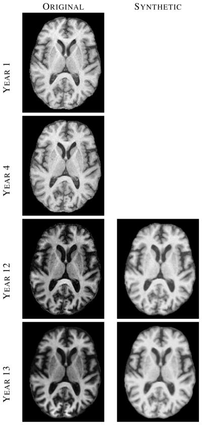
The left column shows images from four (out of fourteen) time-points of a normal BLSA subject, where each image was acquired approximately one year apart. The right column shows synthetic SPGR images, synthesized using MIMECS applied to the corresponding MPRAGE images in the left column.

Since analysis of longitudinal changes in brain volume is the primary objective in the BLSA study (cf. [12]), we used a state-of-the-art longitudinal segmentation algorithm called longitudinal FreeSurfer [71] (longFS) to segment and label the resulting data. LongFS can only be applied to data having the same pulse sequence (either SPGR or MPRAGE), so we were able to apply it to 14 volumes comprising the original 11 SPGR volumes and the 3 MIMECS SPGR volumes. Plots showing the computed GM and ventricle volumes as a function of subject age are shown in Fig. 5 (red with asterisks). For comparison, we applied longFS to each of the longitudinal segments acquired using the same pulse sequence. Accordingly, Fig. 5 also shows the GM and ventricle volumes for the 11 time frames having SPGR (blue with triangles) data and the 3 time frames from both the original MPRAGE (using the -mprage flag in longFS) and the MIMECS SPGRs (pink with crosses and green with squares, respectively).

Fig. 5.

GM and ventricle volumes from longitudinal FreeSurfer [71] of a normal subject with 14 scans (first 11 are SPGR, last 3 are MPRAGE).

The first key observation to make from Fig. 5 is that longFS yields very different segmentation results and corresponding volume measurements given source data with different pulse sequences. Every neuroimage segmentation algorithm that we have ever tested shares this discrepancy, so this observation should not be interpreted as an indictment of longFS. The second key observation is that MIMECS synthesis permits longFS to make very consistent longitudinal segmentations (at least as far as the volume measured from these segmentations) across the entire collection. Even the segmentation results from the short sequence of synthetic SPGRs are more consistent with the older data. Therefore, we conclude that MIMECS may be a useful preprocessing step prior to analysis of volume changes in longitudinal neuroimaging studies.

B. Average atlas construction

While developing voxel based measures from a population, it is common practice to register all the images to an average atlas space. However, pooling data from two populations can be difficult when individual images from two populations are acquired with different pulse sequences or on heterogeneous scanners. In this case study, we show that by synthesizing contrasts using MIMECS, a better average atlas can be created while pooling subjects from two different data sets. This MIMECS case study represents a new capability; the use of multiple data sources in atlas construction enabling richer and more complete analyses.

As a straight forward demonstration of this, we selected five normal subjects from the BLSA database (1.5T GE, SPGR) and five normal subjects from the OASIS [73] databases (1.5T Siemens, MPRAGE), all male and right-handed with age range 60–70 years. A state-of-the-art registration tool SyN [7] was used to create average atlases from these ten subjects. A cross-section and zoomed region of this result are shown in Figs. 6(a) and 6(b). We then synthesized volumes with MPRAGE contrast from the five BLSA subjects and created an average atlas from the ten MPRAGE contrast images. This result and a zoomed region are shown in Figs. 6(c) and 6(d). Visually, the atlas created from all MPRAGE contrasts has sharper features than the one with the mixture of SPGR and MPRAGE contrasts (compare Figs. 6(b) and (d)).

Fig. 6.

(a) Average atlas created using SyN from five BLSA (SPGR) and five OASIS (MPRAGE) images and (b) a zoomed region. (c) Average atlas from five synthetic MPRAGEs from BLSA and five OASIS images (MPRAGE) and (d) a zoomed region. (e) Intensity standard deviation image from SPGR+MPRAGE atlas and (f) intensity standard deviation image from sMPRAGE+MPRAGE atlas.

To show a quantitative improvement in atlas quality, Figs. 6(e) and 6(f) show the voxel-wise standard deviations of intensities from the ten subjects used to create each of the atlases (after deforming them into the atlas space). It can be seen that the standard deviations are much smaller when synthetic MPRAGEs are combined with OASIS MPRAGEs, especially around the ventricles and in the GM, indicating better feature matching in registration. We then segmented the two atlases using TOADS [2]. A t-test shows that the average standard deviations of CSF, ventricles and GM are significantly lower (p-value < 0.01) for the atlas obtained with all MPRAGE contrasts compared to the one obtained with the mixture of SPGR and MPRAGE contrasts. This average atlas construction case study represents an enhancement to existing technologies, which would provide for richer atlas construction and perhaps more accurate deformation fields carrying each subject into the average atlas space (and vice versa).

C. Segmentation bias in cross-sectional analysis

When pooling data from different studies, the choice of scanning protocols introduces algorithm bias in the quantification even the simplest biomarkers, such as GM and WM volume. To study this bias we used 42 age-matched normal subjects (male, right-handed, and 60–70 years of age), 21 from the BLSA database (all SPGR scans) and 21 from the OASIS [73] database (all MPRAGE scans). The images were then skull-stripped [67] and segmented with FreeSurfer [74]. Plots of average ventricle and brain (GM+WM) volume are shown in Fig. 7. It is known that FreeSurfer generally overestimates brain volume when using SPGR data [75], and we observe this same tendency here (Fig. 7(a)). To test the null hypothesis that volumes volumes for each structure are the same, we use a Wilcoxon rank-sum test with a significance level of 0.01. The average brain volumes (GM+WM) computed from the SPGR scans are significantly higher (p-value < 0.01) than the MPRAGE brain volumes. There was no statistically significant difference for the ventricle volumes for the two populations.

Fig. 7.

(a) Brain volume (GM+WM) and (b) ventricle volume computed using FreeSurfer [74] on 21 normal subjects from the BLSA (SPGR) database and 21 normal subjects from the OASIS (MPRAGE) database, as well as on the 21 synthetic MPRAGEs generated from the BLSA SPGR images.

We then used MIMECS (with a BIRN SPGR/MPRAGE atlas, as above) to synthesize MPRAGE contrasts from the SPGR scans and then used FreeSurfer to segment the synthetic scans. As shown in Fig. 7(a), the brain volumes computed this way are comparable to those computed using OASIS/MPRAGE data; the same Wilcoxon rank-sum test shows that the MPRAGE and synthetic MPRAGE come from the same distribution. We also observe that the ventricle volumes do not change in a statistically significant way after synthesis, again, with respect to a Wilcoxon rank-sum test. This case study shows that MIMECS can remove the systemic bias in volumetric analysis arising from scanner and pulse sequence differences in studies that pool multi-site and multi-center data.

D. Distortion correction in b₀ scans

Diffusion MR images are acquired using echo-planar techniques and are geometrically distorted by susceptibility and eddy currents unless corrected [76]. Although eddy current distortion correction can be carried out by consideration of the MR physics and pulse sequence alone, susceptibility causes subject-dependent distortion and is generally carried out retrospectively by deformably registering the b₀ image to a structural image such as a T1-w or T2-w image [77]. The b₀ image—a minimally-weighted diffusion image—has a tissue contrast similar to that of a conventional T2-w spin-echo image, thus making T2-w images the preferred target for distortion correction. But what happens if no T2-w image was acquired as part of the protocol? In this case, the correction might be attempted by registering the b₀ image to the T1-w image, leading generally to an inferior result. Here, we consider an alternative approach using MIMECS.

Figs. 8(c) and 8(e) show an MPRAGE image and a b₀ image, respectively, acquired in the same imaging session of a subject from the Kirby-21 database [64]. The b₀ image shows significant distortion in the anterior portion of the brain. Fig. 8(g) shows the b₀ image after it has been registered to the MPRAGE image using SyN [7] (with mutual information as the similarity metric). By comparing the GM/WM boundary generated by FreeSurfer segmentation of the MPRAGE (see Fig. 8(f)) to the underlying intensities of the registered b₀ image (see Fig. 8(h)), it is clear that the correction is inadequate.

Fig. 8.

(a) and (b) show an atlas pair consisting of MPRAGE and T2-w scans of a normal subject from the Kirby-21 data set. A subject MPRAGE scan (c) is used with MIMECS to synthesize a T2-w image of the subject (d). The acquired subject b₀ image (e) is deformably registered to the subject T1-w image using SyN (with the MI criterion) yielding the corrected image (g). Contours generated from FreeSurfer on the T1-w image (f) are shown on the geometry corrected b₀ image (h). The acquired b₀ image is deformably registered to the synthetic MIMECS image using SyN (CC criterion) to create a MIMECS corrected image (i). Overlaid contours on this image (j) reveal much better geometry correction.

Given the atlas shown in Figs. 8(a) and 8(b), we used MIMECS to synthesize T2-w image from the MPRAGE image; the result is shown in Fig. 8(d). We then registered the b₀ image to the synthetic T2-w using SyN (with the cross-correlation similarity metric), yielding the distortion-corrected b₀ image shown in Fig. 8(i). The red arrow in Fig. 8(i) indicates an area of improvement, which can be visually confirmed on the zoomed region containing the GM/WM contour shown in Fig. 8(j).

This case study demonstrates a potential use of MIMECS in cases where data is missing. It also reveals a new potential approach to registration of multimodal data, wherein synthesis of the alternate tissue contrast is used with a cross-correlation metric rather than the conventional mutual information metric applied to different tissue contrasts. This concept could have far more general applicability than the simple case example demonstrated here.

E. High resolution T2-w synthesis

Because of time constraints, T2-w scans are often acquired at lower resolution than T1-w scans. If high-resolution (hi-res) T2-w scans were available, however, they could be used for many purposes including lesion segmentation [78], [79] and b₀ dewarping (as described in the previous section). Super-resolution techniques using non-local means have previously been proposed to synthesize hi-res T2-w images [38], [80]. These methods use patches from both the hi-res T1-w image and a lo-res T2-w image and index into an atlas comprising these two images and a hi-res T2-w image.

MIMECS provides an alternate way to carry out super-resolution, where the hi-res T2-w image can be synthesized directly from a subject’s high-res T1-w image. This means that acquisition of the lo-res T2-w image is unnecessary (for image processing purposes). As an example, consider the SPGR and T2-w images shown in Figs. 9(a) and 9(b), respectively. Both data sets were acquired axially with native resolutions of 0.94 × 0.94 × 1.5 mm and 0.94 × 0.94 × 5 mm, so the low through-plane resolutions are readily apparent as vertical blurring in both of these coronal images—and, clearly, it is much worse in the T2-w image. We use Brainweb [63] T1-w and T2-w images as the atlas images, a₁ and a₂, as shown in Figs. 9(c) and 9(d), because both are available at high resolution. MIMECS is then used to synthesize a hi-res T2-w image from the SPGR image alone, and the result is shown in Fig. 9(f). For comparison, an upsampled (super-res) result using the non-local means method of [80] is shown in Fig. 9(e). It is readily apparent by visual inspection that MIMECS produces a superior hi-res T2-w image over both the original T2-w acquisition and the non-local means result.

Fig. 9.

Coronal views of (a) SPGR (native resolution 0.94 × 0.94 × 1.5mm) and (b) T2-w (native resolution 0.94 × 0.94 × 5mm) scans of a subject. (The T2-w image has been upsampled to the SPGR resolution using trilinear interpolation.) Brainweb (c) T1-w and (d) T2-w phantoms used as an atlas in MIMECS. (e) A hi-res T2-w image upsampled using a non-local super-resolution method. (f) MIMECS synthesized hi-res T2-w image.

F. MIMECS image segmentation

In this section, we show that MIMECS can also be used as a tissue classification and image segmentation method. In this experiment, we use five atlases, each containing a T1-w SPGR images and its segmentation into CSF, GM, and WM tissue classes. The segmentations, illustrated in the top center of Fig. 10, were carried out by FreeSurfer [74] followed by expert manual corrections.

Fig. 10.

The top row shows a subject T1-w SPGR image, three of the five classification atlases, and fuzzy memberships produced by MIMECS-based tissue classification. Hard segmentations from two leading automatic methods and a manually-corrected method are compared to the hard segmentation of MIMECS.

In order to make use of MIMECS when label images rather than image intensities are involved, we must rethink its steps. Consider a single atlas (an image and its segmentation) and a single voxel (with its corresponding subject patch) in the MIMECS procedure (as described in Section III-B). Determination of the sparse coefficient vector x̂(j), which defines an optimal combination of atlas patches that best match the subject patch (see (5)), can be carried out as usual. But to use this vector to form a linear combination of label patches as in (4) does not make sense since the labels are discrete quantities. Two simple modifications are needed to solve this problem.

First, we form the contrast dictionary A₂ as usual; it comprises a single patch in each column and each patch is a collection of labels from a₂. Let us represent the labels as follows: CSF (k = 1), GM (k = 2), and WM (k = 3). We now form a vector contrast dictionary ${\mathbf{A}}_2=(A_2^1,A_2^2,A_2^3)$ with its elements defined by

$$A_2^k=\{\begin{array}{ll}1\hfill & \text{if}{A}_2=k\hfill \\ 0\hfill & \text{otherwise}\hfill \end{array}k=1,2,3.$$ (7)

This process is equivalent to viewing the a₂ dictionary image as a vector membership function rather than a label image. The elements of this dictionary are now interpreted as vector membership functions and we are free to form convex combinations of these vectors in order to produce new (fuzzy) membership functions.

This leads us to the second modification of the usual MIMECS process. It is desirable for the linear combination of vector membership functions to be convex combinations; in this way the elements of the resultant membership function will add up to unity and can also be viewed as either probabilities or partial fractions of the tissue classes. Since the elements of x̂(j) are non-negative, we can guarantee its use in making a convex combination by simply dividing the inner products by the sum of the elements of x̂(j). Accordingly, we form a MIMECS-based membership function as follows

$${\mu }_k(j)=\frac{A_2^k\widehat{\mathbf{x}}(j)}{{\Vert \widehat{\mathbf{x}}(j)\Vert }_1},k=1,2,3.$$ (8)

The result of this whole process is a fuzzy tissue classification at each voxel and therefore a fuzzy (or soft) segmentation of the subject image. We have found that the result produced with just one atlas is not highly accurate. To produce a more robust result, we apply this exact approach to five atlases and average the resulting membership functions at each voxel. To produce a hard classification—as in the segmentations that are used in the atlas—we use the conventional maximum membership criterion.

An example of the MIMECS tissue segmentation process is shown in Fig. 10. Note that the membership functions (upper right) look very much like the soft segmentations produced by fuzzy C-means or mixture model methods; they can be used exactly as one might use such functions in subsequent segmentation or analysis stages. A hard segmentation is shown on the bottom right. Hard segmentations from SPM, fully-automatic FreeSurfer (with default parameters), and manually-corrected FreeSurfer are shown for comparison (see bottom row). The MIMECS segmentation has many desirable visual features and compares quite favorably to the manually-assisted FreeSurfer result.

For quantitative comparison, Dice coefficients for the SPM, fully-automatic FreeSurfer, and MIMECS results against the manually-corrected FreeSurfer result were computed, yielding 0.8630, 0.8811, 0.8837, respectively. MIMECS shows a small improvement in this example. The most important point to be made is that this MIMECS segmentation approach does not rely on any statistical (spatial or intensity) prior. Instead it obtains its result through the use of dictionary examples alone. Similar methods in the literature (e.g., [39], [81]–[83]) are gaining wide support because of their superior performance and generalizability in comparison to model-based methods.

G. FLAIR synthesis

FLAIR (fluid attenuated inversion recovery) images have become important in detecting lesions in the brain, especially in WM. Many older studies did not use the FLAIR pulse sequence, so image processing algorithms designed to exploit the FLAIR tissue contrast cannot be directly applied. Also, since the FLAIR pulse sequence is very sensitive to patient motion some FLAIR images are “spoiled” by motion artifacts and are also not amenable to image processing algorithms. We therefore carried out a study on the use MIMECS to synthesize FLAIR images.

The atlas we used for this experiment has three images: a₁ has an MPRAGE contrast, a₂ has a T2-w contrast, and a₃ has a FLAIR contrast. Cross-section of the atlas images are shown in the left-hand column of Fig. 11. The goal is to apply MIMECS using two subject images—an MPRAGE image and a T2-w image—to synthesize a FLAIR image. Both the atlas and the subject has WM lesions, so the presence of a unique lesion patch signature in the subject should also be present in the atlas.

Fig. 11.

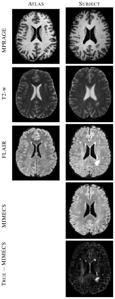
The lefthand column contains an atlas for FLAIR synthesis. The righthand column shows the subject’s true images, a synthetic MIMECS FLAIR image, and a subtraction image (true FLAIR minus synthetic MIMECS FLAIR).

Cross-sections of subject images and the synthetic MIMECS FLAIR image are shown in the right-hand column of Fig. 11. The true FLAIR image for this subject, which is not used in the synthesis algorithm, is shown for comparison. It is immediately evident that the lesions in the synthetic FLAIR image have been rendered as if they are GM—i.e., they are not bright like lesions in true FLAIR images. It is relatively easy to understand why this happens. If one visually identifies a lesion in the (atlas or subject) FLAIR image, it is readily apparent that these same regions on both the MPRAGE and T2-w have intensities that are similar to GM within their respective tissue contrasts. Thus, patches involving lesions in both MPRAGE and T2-w are indistinguishable from patches involving GM.

This experiment reveals a limitation of MIMECS synthesis. Stated simply, the set of pulse sequences used to synthesize a new image must contain intensity signatures that can uniquely identify the tissue classes that are present in the tissue contrast to be synthesized. This is certainly a cautionary note about MIMECS synthesis and it deserves further study to determine its specific limitations. On the other hand, the ability to synthesize images devoid of lesions presents an opportunity to enhance lesions by subtraction. The bottom right image in Fig. 11 is a subtraction image (true subject FLAIR minus synthetic FLAIR) that shows potential for visual enhancement of lesions or for computational assistance in finding lesions.

VI. Summary and Discussion

MIMECS is a new approach to image intensity normalization and tissue contrast synthesis. It is based on sparse dictionary reconstruction methods with a novel patch normalization approach that makes dictionary selection straightforward. For each voxel, a dictionary is found by casting all patches into one higher dimension and searching for “like” patches using a rapid kd-tree search with the ℓ₂ metric. A sparse and non-negative combination of dictionary patches is found to match the subject patch is found using an ℓ₁ solver. These same coefficients are then used to combine patches in another dictionary that is physically matched to the first dictionary. This process is shown in several provided examples to be capable of providing intensity normalization, tissue contrast synthesis, and tissue segmentation.

MIMECS shares strong similarities to non-local means methods [45], some of which have been applied in the medical imaging community for noise reduction [42], [84], [85], super-resolution [80], and segmentation [39], [41], [81]. Including our earlier conference publications on this topic [47]–[49], [86], MIMECS is the first approach of this class to be proposed and evaluated for contrast synthesis. The use of nonnegative coefficients in combining patches is a important aspect, heretofore not considered, in using the patch-based framework for contrast synthesis. As well, the proposed dictionary selection technique, which uses a higher-dimensional space to normalize patches, is novel and important in practical scenarios since it avoids prior segmentation (as we used in earlier reports) or atlas selection training. Finally, the importance of sparsity was demonstrated in Section IV-C and Fig. 3.

Comparisons with histogram matching methods (cf. [25], [87]) were omitted from this paper for length considerations, but results are included in [65] and previous conference reports [47]–[49]. Histogram matching methods are used in nearly every neuroimage processing pipeline and remain important. In fact, MIMECS depends on a crude histogram matching method (linear normalization to the WM peak) at its outset. But histogram matching has serious limitations. For example, histogram matching in its most basic form changes the intensities of the subject image so that its histogram is exactly equal to that of the target. If a simple tissue classifier (such as the EM algorithm for a Gaussian mixture model) were applied to these two images, then the computed volumes of the corresponding tissue classes would be identical. This process would therefore disguise potential differences in a population of subject images. More sophisticated histogram matching methods have been designed, of course, and their results are more sensible. But the whole approach becomes more suspect as the pulse sequences vary significantly and it is entirely wrong to perform histogram matching between images that have fundamentally different tissue contrasts. MIMECS therefore provides an alternative to histogram matching which does not suffer from these fundamental problems.

Our results demonstrate a collection of potential applications of MIMECS. We particularly emphasize the potential for MIMECS to solve the “missing” or “mis-matched” tissue contrast problem in routine neuroimage processing tasks. For example, the BLSA longitudinal study has been active for so long that the SPGR images that were acquired at 1.5 T on older scanners has been replaced by MPRAGE images that are acquired at 3.0 T on modern scanners. MIMECS offers a straightforward way to carry out consistent volumetric analysis across this large time span. The use of diverse data from multiple institutions and multiple studies creates similar difficulties, as illustrated by our average atlas and segmentation bias examples. These examples showed how MIMECS could be used to synthesize “like” data for potential improvement in the statistical analysis of anatomical shape differences through average atlasing or for merging volumetric analysis of normal subjects for greater power in cross-sectional studies.

The average atlas example demonstrated how registration could be improved by synthesizing images having the same tissue contrast. This was taken a step further with the example involving geometric distortion correction in diffusion MRI. Taken together, these two examples reveal a new approach to multimodal registration, one in which a “proxy” image is synthesized from either the subject or target image and registration is carried out using a simple image similarity criterion such as cross-correlation. This approach deserves further scrutiny since it provides an alternative to the mutual information similarity metric, which is problematic to optimize and often fails to provide accurate results, especially in deformable registration applications.

Super-resolution algorithms, and especially patch-based methods have gained a lot of attention in recent years [81], [83]. The MIMECS framework has strong similarity to other patch-based methods, but offers a twist—direct synthesis of an alternate tissue contrast—that could be advantageous. In fact, it is not difficult to envision putting some of the fundamental notions together, for example, having a multi-resolution atlas within the MIMECS framework. Again, certain elements of the MIMECS framework—non-negative patch combination and patch normalization in a higher-dimensional space—offer immediate advantages.

Use of patches for direct segmentation has been previously reported [81]. The advantages of MIMECS for this purpose are not clearly established in this paper as we did not include a comparison with these particular methods. However, our comparison to established state-of-the-art segmentation algorithms demonstrates a strong potential for its use in this way in the future. Like other patch-based methods, the use of examples rather than generative models may be advantageous when models are difficult to ascertain with precision as is often the case in medical imaging. A key limitation of this approach at present is that it provides only a tissue classification, not a structural labeling. FreeSurfer, to which it is compared subdivides the GM into anatomical structures with labels, a critically important set in many neuroimaging analyses.

Our final experiment involved FLAIR image synthesis, and it provides a cautionary lesson about the limitations of MIMECS. The FLAIR pulse sequence is unique in its ability to reveal WM lesions by nullifying the CSF signal using a 180° inversion recovery pulse. This accentuates the lesion signal relative to all other brain intensities. It is a nonlinear relationship to the signal coming from other pulse sequences because of the inversion recovery step, and this is (partly) what makes it impossible to synthesize using MIMECS directly. Lesions are not invisible in MPRAGE and T2-w images, but they are not distinguishable from GM by intensity and local pattern alone. We note that PD images, typically collected along with the T2-w images, do not help us since the lesions in a PD image also look like GM.

While we did illustrate how synthesizing images containing the absence of lesions could potentially be useful in lesion detection, the question still remains as to whether alternate methods or different source images might make FLAIR synthesis possible. It is also natural to ask what other anatomical features or pathologies might not be synthesized using standard MIMECS techniques and how these omissions might affect subsequent image processing steps such as segmentation and registration.

In summary, our case studies demonstrate the immediate utility of MIMECS for a wide variety of neuroimage processing tasks. There remains a great deal of flexibility in its use, particularly in the choice of atlas and source image(s) and new applications can be expected to be found. MIMECS represents a new class of neuroimage processing methods with a potentially rich future.

References

- 1.Bezdek JC, Hall LO, Clarke LP. Review of MR image segmentation techniques using pattern recognition. Med Physics. 1993;20(4):1033–1048. doi: 10.1118/1.597000. [DOI] [PubMed] [Google Scholar]
- 2.Bazin PL, Pham DL. Topology-preserving tissue classification of magnetic resonance brain images. IEEE Trans Med Imag. 2007 Apr;26(4):487–496. doi: 10.1109/TMI.2007.893283. [DOI] [PubMed] [Google Scholar]
- 3.Roy S, Agarwal H, Carass A, Bai Y, Pham DL, Prince JL. Fuzzy c-means with variable compactness. Intl Sym on Biomed Imag (ISBI) 2008 May;:452–455. doi: 10.1109/ISBI.2008.4541030. [DOI] [PMC free article] [PubMed] [Google Scholar]
- 4.Clark KA, Woods RP, Rottenberg DA, Toga AW, Mazziotta JC. Impact of acquisition protocols and processing streams on tissue segmentation of T1 weighted MR images. NeuroImage. 2006;29(1):185–202. doi: 10.1016/j.neuroimage.2005.07.035. [DOI] [PubMed] [Google Scholar]
- 5.Boesen K, Rehm K, Schaper K, Stoltzner S, Woods R, Lüders E, Rottenberg D. Quantitative comparison of four brain extraction algorithms. NeuroImage. 2004 Jul;22(3):1255–1261. doi: 10.1016/j.neuroimage.2004.03.010. [DOI] [PubMed] [Google Scholar]
- 6.Roy S, Carass A, Bazin PL, Resnick SM, Prince JL. Consistent Segmentation using a Rician Classifier. Medical Image Analysis. 2012;16(2):524–535. doi: 10.1016/j.media.2011.12.001. [DOI] [PMC free article] [PubMed] [Google Scholar]
- 7.Avants BB, Epstein CL, Grossman M, Gee JC. Symmetric diffeomorphic image registration with cross-correlation: evaluating automated labeling of elderly and neurodegenerative brain. Medical Image Analysis. 2008;12(1):26–41. doi: 10.1016/j.media.2007.06.004. [DOI] [PMC free article] [PubMed] [Google Scholar]
- 8.Rohde GK, Aldroubi A, Dawant BM. The adaptive bases algorithm for intensity-based nonrigid image registration. IEEE Trans Med Imag. 2003;22:1470–1479. doi: 10.1109/TMI.2003.819299. [DOI] [PubMed] [Google Scholar]
- 9.Rorden C, Bonilha L, Fridriksson J, Bender B, Karnath H. Age-specific CT and MRI templates for spatial normalization. NeuroImage. 2012;61(4):957–966. doi: 10.1016/j.neuroimage.2012.03.020. [DOI] [PMC free article] [PubMed] [Google Scholar]
- 10.Chen M, Carass A, Bogovic J, Prince P-LBJL. Distance transforms in multi channel MR image registration. Proceedings of SPIE Medical Imaging (SPIE-MI 2011); Lake Buena Vista, FL. February 12–17, 2011; 2011. [DOI] [PMC free article] [PubMed] [Google Scholar]
- 11.Ellingsen LM, Prince JL. Mjolnir: Extending HAMMER using a diffusion transformation model and histogram equalization for deformable image registration. International Journal of Biomedical Imaging. 2009;2009:281615. doi: 10.1155/2009/281615. [DOI] [PMC free article] [PubMed] [Google Scholar]
- 12.Resnick SM, Pham DL, Kraut MA, Zonderman AB, Davatzikos C. Longitudinal Magnetic Resonance Imaging Studies of Older Adults: A Shrinking Brain. Journal of Neuroscience. 2003;23(8):3295–3301. doi: 10.1523/JNEUROSCI.23-08-03295.2003. [DOI] [PMC free article] [PubMed] [Google Scholar]
- 13.Thambisetty M, Wan J, Carass A, An Y, Prince JL, Resnick SM. Longitudinal changes in cortical thickness associated with normal aging. NeuroImage. 2010;52(4):1215–1223. doi: 10.1016/j.neuroimage.2010.04.258. [DOI] [PMC free article] [PubMed] [Google Scholar]
- 14.Querbes O, Aubry F, Pariente J, Lotterie J, Démonet J, Duret V, Puel M, Berry I, Fort J-C, Celsis P and The Alzheimer’s Disease Neuroimaging Initiative. Early diagnosis of Alzheimer’s disease using cortical thickness: impact of cognitive reserve. Brain. 2009;132(8):2036–2047. doi: 10.1093/brain/awp105. [DOI] [PMC free article] [PubMed] [Google Scholar]
- 15.Raz N, Rodrigue KM, Acker JD. Hypertension and the brain: Vulnerability of the prefrontal regions and executive functions. Behavioral Neuroscience. 2003;117(6):1169–1180. doi: 10.1037/0735-7044.117.6.1169. [DOI] [PubMed] [Google Scholar]
- 16.Heckemann RA, Keihaninejad S, Aljabar P, Rueckert D, Hajnal JV, Hammers A and The Alzheimer’s Disease Neuroimaging Initiative. Improving intersubject image registration using tissue-class information benefits robustness and accuracy of multi-atlas based anatomical segmentation. NeuroImage. 2010;51(1):221–227. doi: 10.1016/j.neuroimage.2010.01.072. [DOI] [PubMed] [Google Scholar]
- 17.Unschuld PG, Edden RAE, Carass A, Liu X, Shanahan M, Wang X, Oishi K, Brandt J, Bassett SS, Redgrave GW, Margolis RL, van Zijl PCM, Barker PB, Ross CA. Brain metabolite alterations and cognitive dysfunction in early Huntington’s disease. Movement Disorders. 2012 Jun;27(7):895–902. doi: 10.1002/mds.25010. [DOI] [PMC free article] [PubMed] [Google Scholar]
- 18.Friedman L, Stern H, Brown GG, Mathalon DH, Turner J, Glover GH, Gollub RL, Lauriello J, Lim KO, Cannon T, Greve DN, Bockholt HJ, Belger A, Mueller B, Doty MJ, He J, Wells W, Smyth P, Pieper S, Kim S, Kubicki M, Vangel M, Potkin SG. Test-Retest and Between-Site Reliability in a Multicenter fMRI Study. Human Brain Mapping. 2008 Aug;29(8):958–972. doi: 10.1002/hbm.20440. [DOI] [PMC free article] [PubMed] [Google Scholar]
- 19.Kawas C, Gary S, Brookmeyer R, Fozard J, Zonderman A. Age-specific incidence rates of Alzheimer’s disease: the Baltimore Longitudinal Study of Aging. Neurology. 2000 Jun;54(11):2072–2077. doi: 10.1212/wnl.54.11.2072. [DOI] [PubMed] [Google Scholar]
- 20.Mueller SG, Weiner MW, Thal LJ, Petersen RC, Jack C, Jagust W, Trojanowski JQ, Toga AW, Beckett L. The Alzheimer’s disease neuroimaging initiative. Neuroimaging Clin N Am. 2005 Nov;15(4):869–877. doi: 10.1016/j.nic.2005.09.008. [DOI] [PMC free article] [PubMed] [Google Scholar]
- 21.Walter C, Kruessell M, Gindele A, Brochhagen HG, Gossmann A, Landwehr P. Imaging of renal lesions: evaluation of fast mri and helical ct. Br J Radiol. 2003 Oct;76(910):696–703. doi: 10.1259/bjr/33169417. [DOI] [PubMed] [Google Scholar]
- 22.Bergeest JP, Jäger F. Bildverarbeitung für die Medizin 2008, ser. Informatik Aktuell. ch. 8. Springer; Berlin Heidelberg: 2008. A Comparison of Five Methods for Signal Intensity Standardization in MRI; pp. 36–40. [Google Scholar]
- 23.Jäger F, Nyúl L, Frericks B, Wacker F, Hornegger J. Bildverarbeitung für die Medizin 2008, ser. Informatik Aktuell. ch. 20. Springer; Berlin Heidelberg: 2007. Whole Body MRI Intensity Standardization; pp. 459–463. [Google Scholar]
- 24.Nyúl LG, Udupa JK. On Standardizing the MR Image Intensity Scale. Mag Reson Med. 1999;42(6):1072–1081. doi: 10.1002/(sici)1522-2594(199912)42:6<1072::aid-mrm11>3.0.co;2-m. [DOI] [PubMed] [Google Scholar]
- 25.Nyúl LG, Udupa JK, Zhang X. New Variants of a Method of MRI Scale Standardization. IEEE Trans Med Imag. 2000 Feb;19(2):143–150. doi: 10.1109/42.836373. [DOI] [PubMed] [Google Scholar]
- 26.Madabhushi A, Udupa JK. New methods of MR image intensity standardization via generalized scale. Med Physics. 2006 Sep;33(9):3426–3434. doi: 10.1118/1.2335487. [DOI] [PubMed] [Google Scholar]
- 27.He R, Datta S, Tao G, Narayana PA. Information measures-based intensity standardization of MRI. Intl Conf Engg in Med and Biology Soc. 2008 Aug;:2233–2236. doi: 10.1109/IEMBS.2008.4649640. [DOI] [PubMed] [Google Scholar]
- 28.Christensen JD. Normalization of brain magnetic resonance images using histogram even-order derivative analysis. Mag Reson Im. 2003 Sep;21(7):817–820. doi: 10.1016/s0730-725x(03)00102-4. [DOI] [PubMed] [Google Scholar]
- 29.Weisenfeld NL, Warfield SK. Normalization of Joint Image-Intensity Statistics in MRI Using the Kullback-Leibler Divergence. Intl Symp on Biomed Imag (ISBI) 2004 Apr;1:101–104. [Google Scholar]
- 30.Ellingsen LM, Prince JL. Mjolnir:Extending HAMMER Using a Diffusion Transformation Model and Histogram Equalization for Deformable Image Registration. Int J Biomed Imaging. 2009;2009(281615) doi: 10.1155/2009/281615. [DOI] [PMC free article] [PubMed] [Google Scholar]
- 31.Dai Y, Wang Y, Wang L, Wu G, Shi F, Shen D and Alzheimer’s Disease Neuroimaging Initiative, . aBEAT: A Toolbox for Consistent Analysis of Longitudinal Adult Brain MRI. PLoS One. 2012;8(4):60344. doi: 10.1371/journal.pone.0060344. [DOI] [PMC free article] [PubMed] [Google Scholar]
- 32.Han X, Fischl B. Atlas Renormalization for Improved Brain MR Image Segmentation Across Scanner Platforms. IEEE Trans Med Imag. 2007;26(4):479–486. doi: 10.1109/TMI.2007.893282. [DOI] [PubMed] [Google Scholar]
- 33.Fischl B, Salat DH, van der Kouwe AJW, Makris N, Ségonne F, Quinn BT, Dale AM. Sequence-independent segmentation of magnetic resonance images. NeuroImage. 2004;23(Suppl 1):S69–84. doi: 10.1016/j.neuroimage.2004.07.016. [DOI] [PubMed] [Google Scholar]
- 34.Prince JL, Tan Q, Pham DL. Optimization of MR Pulse Sequences for Bayesian Image Segmentation. Med Physics. 1995 Oct;22(10):1651–1656. doi: 10.1118/1.597425. [DOI] [PubMed] [Google Scholar]
- 35.Deichmann R, Good CD, Josephs O, Ashburner J, Turner R. Optimization of 3-D MP-RAGE Sequences for Structural Brain Imaging. NeuroImage. 2000 Jul;12(1):112–127. doi: 10.1006/nimg.2000.0601. [DOI] [PubMed] [Google Scholar]
- 36.Miller MI, Christensen GE, Amit Y, Grenander U. Mathematical textbook of deformable neuroanatomies. Proc Natl Acad Sci. 1993 Dec;90(24):11 944–11 948. doi: 10.1073/pnas.90.24.11944. [DOI] [PMC free article] [PubMed] [Google Scholar]
- 37.Sabuncu MR, Yeo BTT, Van Leemput K, Fischl B, Golland P. A generative model for image segmentation based on label fusion. IEEE Trans Med Imag. 2010;29(10):1714–1729. doi: 10.1109/TMI.2010.2050897. [DOI] [PMC free article] [PubMed] [Google Scholar]
- 38.Rousseau F. Brain Hallucination. Proc. of the 10th European Conf. on Comp. Vision; 2008. pp. 497–508. [Google Scholar]
- 39.Coupé P, Eskildsen SF, Manjn JV, Fonov VS, Collins DL and the Alzheimer’s disease Neuroimaging Initiative, . Simultaneous segmentation and grading of anatomical structures for patient’s classification: application to Alzheimer’s disease. NeuroImage. 2012;59(4):3736–3747. doi: 10.1016/j.neuroimage.2011.10.080. [DOI] [PubMed] [Google Scholar]
- 40.Buades A, Coll B, Morel JM. A Non-Local Algorithm for Image Denoising. IEEE Comp Vision and Patt Recog. 2005;2:60–65. [Google Scholar]
- 41.Hu S, Coupé P, Pruessner JC, Collins DL. Nonlocal regularization for active appearance model: Application to medial temporal lobe segmentation. Human Brain Mapping. 2012;00(00):00. doi: 10.1002/hbm.22183. [DOI] [PMC free article] [PubMed] [Google Scholar]
- 42.Kervrann C, Boulanger J, Coupé P. Bayesian Non-local Means Filter, Image Redundancy and Adaptive Dictionaries for Noise Removal. Proc. of 1st international conference on Scale Space and Variational Methods in Comp. Vision; 2007. pp. 520–532. [Google Scholar]
- 43.Yang J, Wright J, Huang TS, Ma Y. Image Super-Resolution Via Sparse Representation. IEEE Trans Imag Proc. 2010 Nov;19(11):2861–2873. doi: 10.1109/TIP.2010.2050625. [DOI] [PubMed] [Google Scholar]
- 44.Candes EJ, Romberg JK, Tao T. Stable signal recovery from incomplete and inaccurate measurements. Comm on Pure and Appl Math. 2006 Aug;59(8):1207–1223. [Google Scholar]
- 45.Mairal J, Bach F, Ponce J, Sapiro G, Zisserman A. Non-local sparse models for image restoration. IEEE Intl Conf on Comp Vision. 2009:2272–2279. [Google Scholar]
- 46.Elad M, Aharon M. Image Denoising Via Sparse and Redundant Representations Over Learned Dictionaries. IEEE Trans Imag Proc. 2006;15(12):3736–3745. doi: 10.1109/tip.2006.881969. [DOI] [PubMed] [Google Scholar]
- 47.Roy S, Carass A, Prince JL. A Compressed Sensing Approach For MR Tissue Contrast Synthesis. Inf Proc in Med Imaging (IPMI) 2011:371–383. doi: 10.1007/978-3-642-22092-0_31. [DOI] [PMC free article] [PubMed] [Google Scholar]
- 48.Roy S, Carass A, Prince JL. Synthesizing MR contrast and resolution through a patch matching technique. Proceedings of SPIE Medical Imaging (SPIE); 2010. p. 7623. [DOI] [PMC free article] [PubMed] [Google Scholar]
- 49.Roy S, Carass A, Prince JL. Compressed sensing based intensity non-uniformity correction. Intl Sym on Biomed Imag (ISBI) 2011 Apr;:101–104. doi: 10.1109/ISBI.2011.5872364. [DOI] [PMC free article] [PubMed] [Google Scholar]
- 50.Mairal J, Sapiro G, Elad M. Learning Multiscale Sparse Representations for Image and Video Restoration. Multiscale Model Simul. 2008;7(1):214–241. [Google Scholar]
- 51.Elad M, Feuer A. Restoration of a Single Superresolution Image from Several Blurred, Noisy, and Undersampled Measured Images. IEEE Trans Imag Proc. 1997;6(12):1646–1658. doi: 10.1109/83.650118. [DOI] [PubMed] [Google Scholar]
- 52.Aharon M, Elad M, Bruckstein A. K-SVD: An Algorithm for Designing Overcomplete Dictionaries for Sparse Representation. IEEE Trans Sig Proc. 2006;54(11):4311–4322. [Google Scholar]
- 53.Kwatra V, Schödl A, Essa I, Turk G, Bobick A. Graphcut Textures: Image and Video Synthesis Using Graph Cuts. ACM Trans on Graphics. 2003;22(3):277–286. [Google Scholar]
- 54.Hertzmann A, Jacobs CE, Oliver N, Curless B, Salesin DH. Image analogies. Proc. of 28th Ann. Conf. on Comp. Graphics and Interactive Techniques, ser. SIGGRAPH ’01; 2001. pp. 327–340. [Google Scholar]
- 55.Donoho DL. For most large underdetermined systems of linear equations, the minimal ℓ1-norm near-solution approximates the sparsest near-solution. Communications on Pure and Applied Mathematics. 2006;59(7):907–934. [Google Scholar]
- 56.Tibshirani R. Regression Shrinkage and Selection via the Lasso. Journal of Royal Stat Soc Series B (Methodological) 1996;58(1):267–288. [Google Scholar]
- 57.Donoho DL, Tanner J. Sparse Nonnegative Solution of Underde-termined Linear Equations by Linear Programming. Proc Natl Acad Sci. 2005;102(27):9446–9451. doi: 10.1073/pnas.0502269102. [DOI] [PMC free article] [PubMed] [Google Scholar]
- 58.Koh K, Kim S, Boyd S. An interior-point method for large-scale l1-regularized logistic regression. Journal of Machine Learning Research. 2007;8:1519–1555. [Google Scholar]
- 59.Grant M, Boyd S. Recent Advances in Learning and Control, ser. Lecture Notes in Control and Information Sciences. Springer-Verlag Limited; 2008. Graph implementations for nonsmooth convex programs; pp. 95–110. [Google Scholar]
- 60.Elad M, Milanfar P, Rubinstein R. Analysis versus synthesis in signal priors. Inverse Problems. 2007;23(3):947968. [Google Scholar]
- 61.Seeger MW. Bayesian Inference and Optimal Design for the Sparse Linear Model. Journal of Machine Learning Research. 2008;9:759–813. [Google Scholar]
- 62.Friedman JH, Bentley JL, Finkel RA. An Algorithm for Finding Best Matches in Logarithmic Expected Time. ACM Trans on Mathematical Software. 1977;3(3):209–226. [Google Scholar]
- 63.Cocosco CA, Kollokian V, Kwan RKS, Evans AC. BrainWeb: Online Interface to a 3D MRI Simulated Brain Database. NeuroImage. 1997;5(4):S425. [Google Scholar]
- 64.Landman BA, Huang AJ, Gifford A, Vikram DS, Lim IL, Farrell JAD, Bogovic JA, Hua J, Chen M, Jarso S, Smith SA, Joel S, Mori S, Pekar JJ, Barker PB, Prince JL, van Zijl PCM. Multi-parametric neuroimaging reproducibility: A 3-T resource study. NeuroImage. 2011;54(4):2854–2866. doi: 10.1016/j.neuroimage.2010.11.047. [DOI] [PMC free article] [PubMed] [Google Scholar]
- 65.Roy S. PhD dissertation. Johns Hopkins University; 2013. MR Image Contrast Synthesis for Consistent Segmentation. [Online]. Available: http://iacl.ece.jhu.edu/~roy/roythesisjhu2013.pdf. [Google Scholar]
- 66.Carass A, Wheeler MB, Cuzzocreo J, Bazin P-L, Bassett SS, Prince JL. A Joint Registration and Segmentation Approach to Skull Stripping. Intl Sym on Biomed Imag (ISBI) 2007 Apr;:656–659. [Google Scholar]
- 67.Carass A, Cuzzocre J, Wheeler MB, Bazin PL, Resnick SM, Prince JL. Simple paradigm for extra-cerebral tissue removal: Algorithm and analysis. NeuroImage. 2011;56(4):1982–1992. doi: 10.1016/j.neuroimage.2011.03.045. [DOI] [PMC free article] [PubMed] [Google Scholar]
- 68.Sled JG, Zijdenbos AP, Evans AC. A non-parametric method for automatic correction of intensity non-uniformity in MRI data. IEEE Trans Med Imag. 1998;17(1):87–97. doi: 10.1109/42.668698. [DOI] [PubMed] [Google Scholar]
- 69.Moghekar A, Kraut M, Elkins W, Troncoso J, Zonderman AB, Resnick SM, O’Brien RJ. Cerebral white matter disease is associated with Alzheimer pathology in a prospective cohort. Alzheimer’s & Dementia. 2012;8(5):S71–S77. doi: 10.1016/j.jalz.2012.04.006. [DOI] [PMC free article] [PubMed] [Google Scholar]
- 70.Xue Z, Shen D, Davatzikos C. CLASSIC: Consistent Longitudinal Alignment and Segmentation for Serial Image Computing. NeuroImage. 2006;30(2):388–399. doi: 10.1016/j.neuroimage.2005.09.054. [DOI] [PubMed] [Google Scholar]
- 71.Reuter M, Schmansky NJ, Rosas HD, Fischl B. Within-Subject Template Estimation for Unbiased Longitudinal Image Analysis. NeuroImage. 2012;61(4):1402–1418. doi: 10.1016/j.neuroimage.2012.02.084. [DOI] [PMC free article] [PubMed] [Google Scholar]
- 72.Roy S, Carass A, Prince JL. Longitudinal Intensity Normalization of Magnetic Resonance Images using Patches. Proceedings of SPIE Medical Imaging (SPIE-MI 2013); Lake Buena Vista, FL. February 9–14, 2013; 2013. p. 86691J. [DOI] [PMC free article] [PubMed] [Google Scholar]
- 73.Marcus DS, Wang TH, Parker J, Csernansky JG, Morris JC, Buckner RL. Open Access Series of Imaging Studies (OASIS): cross-sectional MRI data in young, middle aged, nondemented, and demented older adults. Journal of Cognitive Neuroscience. 2007 Sep;19(9):1498–1507. doi: 10.1162/jocn.2007.19.9.1498. [DOI] [PubMed] [Google Scholar]
- 74.Dale AM, Fischl B, Sereno MI. Cortical Surface-Based Analysis I: Segmentation and Surface Reconstruction. NeuroImage. 1999;9(2):179–194. doi: 10.1006/nimg.1998.0395. [DOI] [PubMed] [Google Scholar]
- 75.Klauschen F, Goldman A, Barra V, Meyer-Lindenberg A, Lundervold A. Evaluation of Automated Brain MR Image Segmentation and Volumetry Methods. Human Brain Mapping. 2009;30(4):1310–1327. doi: 10.1002/hbm.20599. [DOI] [PMC free article] [PubMed] [Google Scholar]
- 76.Jezzard P, Balaban RS. Correction for geometric distortion in echo planar images from B0 field variations. Mag Reson Med. 1995;34(1):65–73. doi: 10.1002/mrm.1910340111. [DOI] [PubMed] [Google Scholar]
- 77.Ardekani S, Sinha U. Geometric distortion correction of high-resolution 3T diffusion tensor brain images. Mag Reson Med. 2005;54(5):1163–1171. doi: 10.1002/mrm.20651. [DOI] [PubMed] [Google Scholar]
- 78.Souplet J, Lebrun C, Ayache N, Malandain G. An Automatic Segmentation of T2-FLAIR Multiple Sclerosis Lesions. Multiple Sclerosis Lesion Segmentation Challenge Workshop (MICCAI 2008 Workshop); 2008. [Google Scholar]
- 79.Wu Y, Warfield SK, Tan IL, Wells WM, Meier DS, van Schijndel RA, Barkhof F, Guttmann CRG. Automated segmentation of multiple sclerosis lesion subtypes with multichannel MRI. NeuroImage. 2006;32(3):1205–1215. doi: 10.1016/j.neuroimage.2006.04.211. [DOI] [PubMed] [Google Scholar]
- 80.Manjon JV, Coupé P, Buades A, Fonovan V, Collins DL, Robles M. Non-Local MRI Upsampling. Medical Image Analysis. 2010;14(2):784–792. doi: 10.1016/j.media.2010.05.010. [DOI] [PubMed] [Google Scholar]
- 81.Coupé P, Manjon JV, Pruessner J, Robles M, Fonov V, Collins DL. Patch-based segmentation using expert priors: Application to hippocampus and ventricle segmentation. NeuroImage. 2011;54(2):940–954. doi: 10.1016/j.neuroimage.2010.09.018. [DOI] [PubMed] [Google Scholar]
- 82.Eskildsen SF, Coupé P, Fonov V, Manjon JV, Leung KK, Guizard N, Wassef SN, Ostergaard LR, Collins DL and The Alzheimer’s Disease Neuroimaging Initiative, . BEaST: Brain extraction based on nonlocal segmentation technique. NeuroImage. 2012;59(3):2362–2373. doi: 10.1016/j.neuroimage.2011.09.012. [DOI] [PubMed] [Google Scholar]
- 83.Rousseau F, Habas PA, Studholme C. A Supervised Patch-Based Approach for Human Brain Labeling. IEEE Trans Med Imag. 2011;30(10):1852–1862. doi: 10.1109/TMI.2011.2156806. [DOI] [PMC free article] [PubMed] [Google Scholar]
- 84.Manjón JV, Carbonell-Caballero J, Lull JJ, Garcia-Marti G, Marti-Bonmati L, Robles M. MRI denoising using non-local means. Medical Image Analysis. 2008;12(4):514–523. doi: 10.1016/j.media.2008.02.004. [DOI] [PubMed] [Google Scholar]
- 85.Wiest-Daessle N, Prima S, Coupé P, Morrissey SP, Barillot C. Rician noise removal by non-Local Means filtering for low signal-to-noise ratio MRI: applications to DT-MRI. Med Image Comp and Comp Asst Intervention (MICCAI) 2008;11:171–179. doi: 10.1007/978-3-540-85990-1_21. [DOI] [PMC free article] [PubMed] [Google Scholar]
- 86.Roy S, Carass A, Shiee N, Pham DL, Prince JL. MR Contrast Synthesis for Lesion Segmentation. Intl Sym on Biomedical Imaging. 2010:932–935. doi: 10.1109/ISBI.2010.5490140. [DOI] [PMC free article] [PubMed] [Google Scholar]
- 87.Wang L, Lai H, Barker GJ, Miller DH, Tofts PS. Correction for variations in MRI scanner sensitivity in brain studies with histogram matching. Mag Reson Med. 1998 Feb;39(2):322–327. doi: 10.1002/mrm.1910390222. [DOI] [PubMed] [Google Scholar]