Identification of important regressor groups, subgroups and individuals via regularization methods: application to gut microbiome data

Abstract

Motivation: Gut microbiota can be classified at multiple taxonomy levels. Strategies to use changes in microbiota composition to effect health improvements require knowing at which taxonomy level interventions should be aimed. Identifying these important levels is difficult, however, because most statistical methods only consider when the microbiota are classified at one taxonomy level, not multiple.

Results: Using L₁ and L₂ regularizations, we developed a new variable selection method that identifies important features at multiple taxonomy levels. The regularization parameters are chosen by a new, data-adaptive, repeated cross-validation approach, which performed well. In simulation studies, our method outperformed competing methods: it more often selected significant variables, and had small false discovery rates and acceptable false-positive rates. Applying our method to gut microbiota data, we found which taxonomic levels were most altered by specific interventions or physiological status.

Availability: The new approach is implemented in an R package, which is freely available from the corresponding author.

Contact: tpgarcia@srph.tamhsc.edu

Supplementary information: Supplementary data are available at Bioinformatics online.

1 INTRODUCTION

With improved culture-independent techniques, a typical study of gut microbiota now involves data from numerous microbes. The microbes are classified at multiple taxonomy levels, namely, phylum, class, order, family, genus and species. Each taxonomy level has many subdivisions, and the number of subdivisions increase on progression from phylum to species level. Strategies to use changes in microbiota composition to effect health improvements require knowing at which taxonomy level interventions should be aimed. Levels to target are those with subdivisions identified as having an impact on the target health outcome. From a biological perspective, only a few subdivisions at each level are believed to play a role in certain health outcomes. Identifying the few important subdivisions at each level is difficult, however, because of the increasing number of subdivisions on progression from phylum to species level and because the microbial data are typically based on small sample sizes. Thus, a method that overcomes these difficulties and identifies important subdivisions at multiple taxonomy levels is needed.

This biological problem corresponds to a variable selection problem where the variables are grouped at multiple levels, and the number of variables (p) far exceeds the sample size (n). We suppose that each level has sparse effects. In the microbiota data, sparse effects mean that only a few subdivisions within a particular taxonomy level actually impact the health phenotypes of interest. For our purposes, we consider the case where variables are divided into groups and subgroups within the groups. Our interest, thus, is developing a method that selects important groups (e.g. phyla), subgroups (e.g. families) and individual predictors (e.g. genera).

Selecting variables clustered into groups and subgroups is challenging. When the variables are divided only into groups (without subgroups), a popular technique is the group Lasso (Yuan and Lin, 2006), which selects an entire group of variables to be included or excluded from the model. The group Lasso, however, has substantial drawbacks. First, the method assumes that the model submatrices for each group are orthonormal. When orthonormality is not satisfied, the group Lasso may select an incorrect model (Friedman et al., 2010). Second, the group Lasso does not achieve sparsity within each group, which can be useful. For the microbial data, we could design more specific strategies for changing microbiota composition if we knew which particular families (i.e. subgroups) in phyla (i.e. group) impacted health phenotypes of interest.

To overcome the deficiencies of the group Lasso, Simon et al. (2012) recently proposed the sparse-group Lasso (SGL). The method imposes no orthonormality requirements on the group model submatrices and achieves sparsity between and within groups through a clever use of the Nesterov (2007) method for generalized gradient descent. The SGL works well when variables are clustered into groups, but not when they are clustered at more than one level—a feature inherent to gut microbiota data.

To accommodate selecting important groups, subgroups and individual predictors, we propose three new algorithms. The first algorithm, the sparse group-subgroup Lasso (SGSL), generalizes the work of Simon et al. (2012). It is based on using L₁ and L₂ regularizations in a linear regression model; convex non-linear regression models are discussed in the Supplementary Material. Our two other proposed algorithms use appropriate combinations of already existing variable selection procedures. First, we propose applying the group Lasso to the groups followed by SGL applied to the subgroups. Second, we propose applying the group Lasso to both the groups and subgroups followed by applying the Lasso (Tibshirani, 1996) to select among the individual predictors. We demonstrate in a simulation study that our first algorithm outperforms the other two.

SGSL is a special case of the tree-structured group Lasso (Jenatton et al., 2011; Liu and Ye, 2010; Zhao et al., 2009), where nodes on the tree represent groups or subgroups of features and ‘leaf’ nodes represent individual features. The tree-structured group Lasso, however, uses a smoothing proximal gradient method (Kim and Xing, 2012) to ‘prune’ the entire tree collectively, whereas our method uses an accelerated generalized gradient descent approach to determine sparsity among groups, then subgroups and then individual features. Moreover, we consider a tree without cycles, meaning there is no overlap between groups/subgroups of features; i.e. each individual feature only belongs to one subgroup, and each subgroup only belongs to one group. Hence, our problem differs from the overlapping group Lasso as in the analysis of breast cancer gene expression data (Van de Vijver et al., 2002) where the interest is finding important pathways among overlapping genes. Our problem also differs from a hierarchical variable selection (Zhao et al., 2009) where a feature is subject to selection only after another feature is selected first. We do not impose this requirement.

Like other Lasso-based procedures, SGSL also requires selecting tuning parameters, for which we propose a data-adaptive approach. Our approach involves multiple applications of 10-fold cross-validation that we show performs well in selecting the tuning parameters through various simulation studies. Therefore, the main contributions from our work include (i) a new variable selection procedure (SGSL), which identifies important groups, subgroups and individual predictors through combined L₁ and L₂ regularizations. (ii) We show that achieving sparsity at multiple levels cannot be achieved through simple combinations of existing Lasso approaches. We show that such combinations will select relevant features less often than SGSL or never (Section 3). (iii) We provide a data-adaptive cross-validation approach that improves over the traditional cross-validation to select the tuning parameters. (iv) In microbiome data, our method identifies which taxonomic levels were most altered by specific interventions or physiological status.

The rest of the article is as follows. Section 2 describes SGSL and Section 3 evaluates its performance compared with competing methods. In Section 4, we describe the microbiota data that motivated this methodology and analyze the data. Section 5 concludes the article.

2 METHODS

2.1 Data structure

We consider a linear regression model with sample size n, a response variable across the samples, and an matrix of predictors . For the microbial data, corresponds to measurements of health features, and contains information about the p microbes. We have , and without loss of generality, all variables are standardized to have mean zero and sample variance one, so that the intercept is excluded from the model.

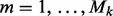
Because the predictors have subgroup and group memberships, we suppose there are L disjoint groups, and each group k has M_k disjoint subgroups, . By the disjointedness assumption, there is no overlap between groups, or overlap between subgroups.

We assume that group k contains p_k predictors denoted by the matrix . We also assume that subgroup m in group k contains predictors denoted by the matrix . The notation is such that refers to the predictors in group k; whereas refers to the predictors in subgroup m of group k. The total number of predictors across all subgroups in group k is p_k (i.e. ), and the total number of predictors across all groups is p (i.e. ). 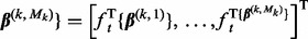Finally, denotes the coefficient vector associated with group k, and is associated with subgroup m in group k.

2.2 New criterion for achieving sparsity among groups, subgroups and individual predictors

2.2.1 SGSL: extension of the SGL

Our primary objective is identifying the relevant groups, subgroups and individual predictors in relation to . Doing so involves finding a sparse solution for the coefficient values; i.e. some coefficient values will be zero and some will be non-zero. If a group’s (subgroup’s) coefficient vector is all non-zero, then that group (subgroup) is relevant. Otherwise, if there is a mix of zero and non-zero coefficients in a subgroup, then those predictors with non-zero coefficient values are relevant and those predictors with zero coefficient values are not.

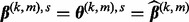
To determine which coefficient values are zero and non-zero, we propose solving where

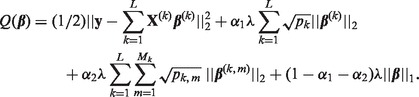Here, denotes the L₂-norm and denotes the L₁-norm. The regularization parameters and control the level of sparsity among the groups, subgroups and individual predictors, and satisfy two criteria: and . Sparsity among groups and subgroups results from the non-differentiability of the L₂-norm at zero. For example, because is non-differentiable at , the group coefficient can be exactly zero. Likewise, the subgroup coefficient can be exactly zero because is non-differentiable at . Though we define for a linear model, our method also extends to convex non-linear regression models; see the Supplementary Material.

The criterion also encompasses different versions of the Lasso. We have the Lasso (Tibshirani, 1996) at ; the group Lasso (Yuan and Lin, 2006) at ; the group Lasso at the subgroup level at ; SGL (Simon et al., 2012) among groups at ; SGL among subgroups at ; and we have sparsity only among groups and subgroups when and .

To find the minimizer of , we take advantage of the criterion’s convexity and separability between groups and subgroups. Through a careful analytical derivation involving properties of subgradients and the Karush–Kuhn–Tucker conditions, we derive the conditions for when the group coefficient and the subgroup coefficient are exactly zero; see Supplementary Material. These results motivate us to use a blockwise descent algorithm at the group and subgroup levels. When a subgroup’s coefficient vector is non-zero, we estimate the subgroup coefficients using the accelerated generalized gradient descent method (Nesterov, 2007) and a step-size optimization as in Simon et al. (2012).

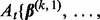
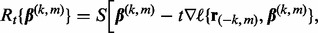
In the algorithm below, let denote the partial residual after removing group k, and denote the partial residual after removing subgroup m from group k. Let be the coordinate-wise soft thresholding operator (Donoho and Johnston, 1994): where . Let , and define as well as .

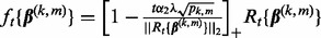Our proposed algorithm is then:

• 1. Group component: Iterate through each group . If for group k,

  (1)

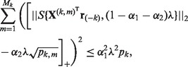
  set ; otherwise, and do step 2 for group k.
• 2. Subgroup component: Iterate through the subgroups of group k and do the following.

  • a. If , set . Otherwise, , and do step (b).
  • b. Set the step-size t = 1 and counter s = 1. Define and

    

    Let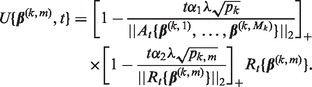 , where is the current value. Iterate through the following steps until convergence:

    • (1) Compute the gradient .
    • (2) Compute .
    • (3) If update the step size t to . Repeat until the inequality no longer holds to optimize t.
    • (4) Set as .
    • (5) Set as ; i.e. a Nesterov step.
    • (6) Update s to s + 1.

The algorithm above, known as SGSL, generalizes the SGL algorithm. When the predictors are divided only into groups (i.e. ), the above algorithm is actually distinctly different from SGL. This is because of the definition of in Step 2(b), which uses information from subgroups and groups, not just groups. When , the condition in Equation (1) is equivalent to when an entire group is excluded from the model in SGL (Simon et al., 2012).

2.2.2 Selection of regularization parameters

Different choices of yield different solutions . To select these tuning parameters, we proceed as follows.

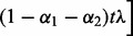
First, for a fixed , we choose the optimal λ by varying it over the range , where is the smallest λ such that is minimized at , and τ is a small fraction, such as 0.05. To find , note that from condition (1), minimizes when

(2)

for all groups . Thus, is the smallest λ value where the above inequality holds for all groups. A practical approach for approximating is taking for , and stopping at the first j for which condition (2) holds for all groups. At this first j, we have that 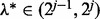. To further improve the estimate of , one may then bisect the interval repeatedly until , where . Here, when , condition (2) holds for all groups, and when , condition (2) fails to hold for at least one group. Finally, take .

Performing the algorithm in Section 2.2.1 at fixed and over the range of λ values yields different model fits. Among all fits, we choose the best descriptive model as the one that minimizes Mallows’ C_p criterion: , where denotes the number of predictors in the selected model, denotes the residual sum of squares and is an appropriate estimator of the model error variance. For example, when can be the residual mean square when using all available variables, or when can be the variance of (Hirose et al., 2013). Mallows’ C_p criterion balances the residual sum of squares of a fitted model with the number of non-zero parameter estimates. Other model selection criteria may also be used (Müller and Welsh, 2010).

The above procedure selects λ well for a fixed , and now we describe how to optimally select and . We propose selecting the optimal based on repeated 10-fold cross-validation as advocated by Garcia et al. (2013) and Martinez et al. (2011). For a fixed and , a single application of 10-fold cross-validation works as follows: (i) randomly partition the data into 10 non-overlapping equal-sized subsets; (ii) remove data subset d, and apply the algorithm in Section 2.2.1 at and over the range of λ, and select the model that minimizes Mallow’s C_p criterion. The minimizing model has associated solution denoted by (the subscript emphasizes the notion that data subset d was removed); (iii) repeat step (ii) for each data subset and compute the cross-validation score where and denote the response and explanatory variables for the data subset d that was removed and is the solution from step (ii). In our applications, we repeated this three-step procedure for taking values 0.01, 0.04, 0.07, 0.10, 0.15, 0.25, 0.35, 0.45, 0.55, 0.65, 0.75, 0.85, 0.95 such that . The optimal is the pair that minimizes the cross-validation score.

Analogous to the work done in Garcia et al. (2013) and Martinez et al. (2011), we did two additional steps to the above 10-fold cross-validation. First, when the minimizer of the cross-validation score was not unique, we took as the average of the minimizers. Second, because Step (i) yields a different random partition on each application, repeated applications of the 10-fold cross-validation may yield different optimal and thus different selected variables, especially when the signals are sparse and small. Martinez et al. (2011) also noted this and suggested performing the 10-fold cross-validation repeatedly, e.g. 100 times, to develop a complete understanding of the variables selected. The idea, thus, is to repeat the 10-fold cross-validation multiple times and retain those variables that were selected at least 60% of the time, say.

2.3 Repeated application of current Lasso methods

Other possible approaches for obtaining sparsity among groups, subgroups and individual predictors are through appropriate combinations of the Lasso, group Lasso and SGL.

2.3.1 Group Lasso and SGL

To achieve sparsity among the groups, one may first apply the group Lasso after orthonormalizing the group model matrices. The group Lasso criterion is when and in , and hence depends only on the regularization parameter λ. To optimally select λ, we evaluate the criterion with at a range of λ values as in Section 2.2.2. The optimal λ corresponds to the model that minimizes Mallows’ Cp criterion. Because the group Lasso selects an entire group of predictors to be included/excluded from the model, the chosen model will have some groups with all non-zero coefficients (i.e. groups retained by the group Lasso), and some groups with all zero coefficients (i.e. groups dismissed by the group Lasso).

After achieving sparsity among groups, we then proceed to achieve sparsity among the subgroups and individual predictors via SGL. For those groups selected by the group Lasso, we apply SGL to all subgroups within these groups. When applying SGL, we do not orthonormalize the subgroup model matrices as done for the group Lasso. The criterion for SGL among subgroups is when in and thus depends on . We choose the optimal λ and via a repeated 10-fold cross-validation as in Section 2.2.2.

2.3.2 Repeated group Lasso and Lasso

Another way to achieve the desired sparsity is as follows. First, apply the group Lasso to the orthonormalized group model matrices to select relevant groups. Second, using the selected groups, select relevant subgroups within by applying the group Lasso to the orthonormalized subgroup model matrices. Lastly, select relevant individual predictors by applying the Lasso to all predictors in the selected subgroups. In the last step, the Lasso is applied to the original predictors, not the orthonormalized versions. In each application of group Lasso and Lasso, criterion only depends on λ, which is chosen as in Section 2.2.2.

3 SIMULATION STUDY

3.1 Simulation design

We evaluated the performance of the proposed methods in Section 2 on simulated data where predictors have group and subgroup memberships. We considered L = 10 groups such that each group had 2 subgroups. We divided p = 80 predictors so that each subgroup had 4 predictors, and each group had 8 predictors.

Covariates in each group were generated from a distribution where 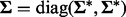and . Here, corresponds to a matrix of ones, and is the identity matrix. This data generation procedure implies that predictors within the same subgroup have a correlation of 0.7, but predictors in different subgroups/groups are independent.

We set sample size n = 30 and generated the response variable 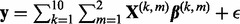, where is 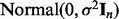. The parameter and the coefficient vectors for each subgroup were chosen according to two settings. In Setting 1, and . All remaining subgroup coefficients were zero. In Setting 2, and . Again, all remaining subgroup coefficients were zero.

For each parameter setting, we generated 500 datasets and applied seven methods: SGSL, the two variable selection procedures in Section 2.2.2 and the following four other competing methods.

1. Lasso: We applied the Least Angle Regression algorithm of Efron et al. (2004), which provides the entire sequence of model fits in the Lasso path. The best fitting model was that which minimized Mallows’ C_p criterion. This method ignores the grouped nature of the predictors.

2. Group Lasso: We applied the group Lasso after orthonormalizing the group model matrices. To find the best fitting model, we minimized , with , over a range of λ values as in Section 2.2.2, and chose the model that minimized Mallows’ C_p criterion. This method yields sparsity among groups, but not among subgroups, nor individual predictors.

3. Repeated group Lasso: We applied the group Lasso at the group and subgroup levels. In each application of the group Lasso, the best fitting model was that which minimized Mallows’ C_p criterion. This method yields sparsity among groups and subgroups, but not among individual predictors.

4. Sparse-group Lasso: We applied SGL among the groups; that is, we minimized where . To select the tuning parameter and λ, we applied the repeated 10-fold cross-validation in Section 2.2.2. This method ignores subgroup memberships and may not select significant subgroups.

For all methods requiring a selection of and/or , we repeated the 10-fold cross-validation 100 times to select the optimal and/or . Ultimately, this led to 100 possibly different values, and thus 100 possibly different ways variables were selected. Ultimately, we retained variables that were chosen at least 60% of the time in the 100 repeated applications. We did not use the average of the values to select the variables.

To evaluate the seven methods, we computed the average percentage of time predictors were selected, the observed false discovery rate (Benjamini and Hochberg, 1995, FDR) and geometric mean of specificity and sensitivity (defined later in the text). To compute these quantities, we divided the predictors in each subgroup into those whose true parameter values are non-zero (i.e. relevant predictors), and those whose true parameter values are zero (i.e. irrelevant predictors). We then reported the average percentage of time relevant and irrelevant predictors were selected in each subgroup. The observed FDR is the ratio of the average number of irrelevant predictors selected (i.e. false selections) over the average number of predictors selected. The geometric mean of sensitivity and specificity is (Kubat et al., 1998). Specificity is the proportion of irrelevant predictors that were not selected among irrelevant predictors, and sensitivity is the proportion of relevant predictors that were selected among relevant predictors. The range of G is [0,1], and large G-values indicate that most predictors are classified correctly. We prefer G over specificity and sensitivity alone, as it counteracts the imbalance between the number of relevant and irrelevant predictors (Kubat et al., 1998). Observed FDR and G-values were computed using all groups, and using only Groups 2 and 3 so as to demonstrate how the methods perform for these two groups, which have sparsity within their subgroups.

Among all methods, the reliable one will routinely select relevant predictors, and rarely or never select irrelevant predictors. Thus, the ideal method will have low FDRs and high G-values.

3.2 Simulation results

Results for the two simulation settings are given in Table 1. In general, our procedure based on the new criterion provided the most reliable results: it largely selected the relevant predictors and ignored irrelevant predictors (irrelevant predictors were incorrectly chosen <5% of the time). This performance resulted in small FDRs, often smaller than the FDRs from other methods. In comparison to SGL, we expected our method to perform equally well when determining relevant groups (both methods have essentially similar criterion for determining if a group is relevant or not), but we expected our method to outperform SGL in detecting sparsity between and within subgroups. SGL is not designed to detect relevant subgroups within a group, nor is it designed to detect relevant individual predictors within a subgroup. Our method, in contrast, can do this. The results from our simulation study confirmed these expectations.

Table 1.

Simulation results for Setting 1 and 2 based on 500 simulations

Group	Subgroup	SGSL	SGL	Lasso	GpL, SGL	GpL × 2, Lasso	GpL × 2	GpL	New method	SGL	Lasso	GpL, SGL	GpL × 2, Lasso	GpL × 2	GpL
		Setting 1							Setting 2
1	1 (Non-zero)	53.20	56.70	40.80	14.10	11.05	20.80	25.20	50.80	52.45	38.85	11.00	9.25	16.80	18.00
	2 (Non-zero)	54.05	56.35	41.50	14.10	12.65	23.00	25.20	52.50	52.95	39.90	11.10	8.20	15.20	18.00
2	1 (Non-zero)	16.55	12.55	13.40	0.00	0.00	0.00	0.00	17.65	12.75	15.45	0.00	0.00	0.00	0.00
	2 (Zero)	4.85	5.45	5.70	0.00	0.00	0.00	0.00	4.90	5.30	5.70	0.00	0.00	0.00	0.00
3	1 (Non-Zero)	19.20	13.60	21.30	0.00	0.00	0.00	0.00	26.50	19.70	25.80	0.00	0.00	0.00	0.00
	1 and 2 (Zero)	3.50	3.37	3.77	0.00	0.00	0.00	0.00	4.40	4.60	4.77	0.00	0.00	0.00	0.00
4–10	(Zero)	0.03	0.01	0.04	0.00	0.00	0.00	0.00	0.04	0.02	0.04	0.00	0.00	0.00	0.00
FDRa		0.07	0.07	0.10	0.00	0.00	0.00	0.00	0.08	0.09	0.11	0.00	0.00	0.00	0.00
Ga		0.64	0.64	0.56	0.30	0.28	0.38	0.41	0.63	0.63	0.56	0.27	0.24	0.33	0.35
FDRb		0.28	0.35	0.32	NA	NA	NA	NA	0.27	0.35	0.31	NA	NA	NA	NA
Gb		0.40	0.35	0.36	0.00	0.00	0.00	0.00	0.41	0.35	0.38	0.00	0.00	0.00	0.00

Note: Average percentages of time each set of variables is selected with our proposed sparse group–subgroup Lasso (‘SGSL’); sparse-group Lasso (‘SGL’); Lasso; group Lasso at group level and sparse-group Lasso at subgroup level (‘GpL, SGL’); group Lasso at group and subgroup levels, and Lasso at individual features level (‘GpL × 2, Lasso’); group Lasso at group and subgroup levels (‘GpL × 2’); and group Lasso (‘GpL’). A ‘non-zero’ subgroup means variables are relevant; a ‘Zero’ subgroup means variables are irrelevant.

^aWe also report observed false discovery rate (FDR) and G-values using all groups.

^bWe also report observed false discovery rate (FDR) and G-values using Groups 2 and 3.

‘NA’ denotes values were incomputable because of division by 0.

Our proposed procedure performed as well as SGL in selecting Group 1, which had all non-zero coefficients. But, our method better detected the true sparsity in Groups 2 and 3. Compared with SGL, our method correctly selected the relevant subgroups and relevant individual predictors at least 4% more often, and had nearly the same or fewer incorrect decisions in selecting irrelevant predictors. This correct classification is evident by the larger G-value for Groups 2 and 3 (see in Table 1). For these two groups, our proposed method has a G-value at least 1.14 times bigger than the G-value for SGL. When considering all groups together (see in Table 1), the G-values for our proposed method and SGL are similar because of the similar performance in Groups 1 and Groups 4–10. This is no surprise given that for Group 1 and Groups 4–10, our proposed method and SGL have similar selection criteria, and thus, should behave equally well as they do. However, when there is sparsity between and within subgroups (as is common in microbiome data; see Section 4), SGL fails to detect such a structure. Thus, when there is sparsity between and within groups and subgroups, our method has higher sensitivity and more power than SGL.

Our proposed method also yielded better results than the other five methods in terms of capturing the true clustering and achieving higher G-values. The Lasso, designed to select individual predictors but not entire subsets, largely ignored the relevant cluster of predictors in Group 1 and in Group 2, subgroup 1. For Group 3, which only had 3 of 10 relevant predictors, the Lasso did successfully select these variables as often as our proposed procedure did. Thus, when necessary, our method can behave similarly to the Lasso, which is an attractive feature when individual features need to be selected. Still, because our simulated data has a specific grouping structure which the Lasso cannot capture, our proposed method has larger G-values than the Lasso both when computed across all groups (0.64 for our method compared with 0.56 for the Lasso) and when computed for Groups 2 and 3 (0.40 for our method compared with 0.36 for the Lasso). Hence, because our interest goes beyond selecting individual predictors, we prefer our proposed method.

Lastly, the proposed iterative procedures all fared poorly, with G-values nearly half that of our proposed method. These iterative methods selected relevant predictors in Group 1 nearly three times less often than did our proposed method and never selected the relevant predictors in Groups 2 and 3. The inability to detect the relevant clusters in Groups 2 and 3 most likely resulted from the initial application of the group Lasso. As the group Lasso is designed to detect relevant groups, it has difficulty determining if an entire group is relevant when that group is sparse. Thus, the sparsity in Groups 2 and 3 prevented the group Lasso, and all forthcoming Lasso-based methods, from selecting these groups or the relevant clusters within.

4 EMPIRICAL EXAMPLE

4.1 Microbial data

Our motivating example is from a dietary treatment study in mice (Thomas et al., 2013) for which we measured fecal microbial diversity. The study used an obesity reversal paradigm and consisted of n = 30 obese male mice equally and randomly assigned to one of three diets: (i) a control soy-based diet with 0.5% (by weight) inorganic calcium; (ii) a high calcium soy-based diet with 1.5% (by weight) inorganic calcium; and (iii) a non-fat dry milk (NFDM) diet with 1.5% (by weight) calcium as NFDM-intrinsic and inorganic calcium. After 10 weeks of feeding, feces from all mice were analyzed for microbial communities via pyrosequencing. Mice on the NFDM diet had enhanced bodyfat loss (Thomas et al., 2013).

For each mouse, data consists of relative messenger RNA (mRNA) expression of CD68 in adipose and microbial percentages () from p = 51 microbes classified at the phylum, family and genus levels. The mRNA expression of CD68 is used to judge the extent to which macrophages have infiltrated adipose, an event that occurs with bodyweight gain and is associated with systemic inflammation (Thomas et al., 2013). The microbes were classified into two phyla: Bacteriodetes and Firmicutes. Each phylum had at least five families, with each family having at least two bacterial genera. The key interest is to find those microbial phyla, families and genera associated with CD68 mRNA expression in this setting.

A prior analysis in Garcia et al. (2013) demonstrated that diet has a significant impact on expression of mRNA for CD68. To accommodate this diet effect, we took the response variable () as the residuals from regressing expression of mRNA for CD68 on diet. See Garcia et al. (2013) for other approaches.

4.2 Results

We applied the same seven variable selection techniques from the simulation study to the microbial data. We found that our proposed procedure selected the entire family Streptococcaceae in the Firmicutes phyla to have an effect on expression of mRNA for CD68. The family consisted of Lactococcus and Streptococcus genera. In comparison, SGL and Lasso were only able to pick one member from this family (Streptococcus), which indicates the inflexibility of these latter two methods in selecting important families (i.e. subgroups).

Having our method select the Streptococcaceae family makes sense, as members of Streptococcaceae flourish in nutrient-rich environments, such as an overfed subject’s gut (e.g. obese mice). Moreover, mice in this study experienced chronic inflammation secondary to obesity and hyperglycemia as evidenced by elevated adipose CD68 arising from macrophage infiltration of adipose tissue (Thomas et al., 2013). At present, it seems unlikely that simple chronic caloric excess promoted Streptococcaceae abundance in the obese mice, as this relationship was not seen in newly obese mice [see Thomas et al. (2012) and Supplementary Material]. Secondary effects appear to play a role as changes in host inflammatory state were previously associated with Streptococcaceae family members in hosts with either strongly positive or negative energy balance. Intestinal infusion of fecal microbiota from lean donors improved glucose metabolism in obese humans with metabolic syndrome in conjunction with a 30% reduction in the Streptococcaceae family member Streptococcus bovis in the small intestine (Vrieze et al., 2012). Obesity driven type II diabetes and metabolic syndrome are considered chronic inflammatory states (Dandona et al., 2005).

In recent studies, the Streptococcaceae family has been shown to be associated with inflammation of various origins and in an energy independent fashion. First, host physiology can influence the composition of the microbiota. For example, poor glucose control in a cohort of European women was associated with Streptococcus sp. C150 (Karlsson et al., 2013). Second, microbiota composition can modulate host physiology in a variable way. For example, formula feeding is associated with increased frequency of pediatric intestinal inflammation including necrotizing enterocolitis; in a mouse model formula feeding increased Lactococcus at the expense of Lactobacillus and altered host gene expression to indicate increased oxidative stress, inflammation and impaired defense capacity (Carlisle et al., 2013). Third, Smith et al. (2013) showed that microbiota composition determines host health outcome in response to identical dietary shifts; in this case, microbiota from twin pairs discordant for the disease Kwashiorkor variably provoke disease depending on the complexity and adequacy of the diet.

Stability and resilience of intestinal microbial diversity is an active area of research, and it is now recognized that chronic alterations in host environmental exposure (e.g. diet) and physiological state (e.g. obese) can influence intestinal microbiota (Lozupone et al., 2012) and likewise microbiota can respond to diet to increase/decrease susceptibility of the host to disease (Carlisle et al., 2013; Smith et al., 2013). Our results further highlight the need to understand temporal dimension of interventions to improve efficacy.

5 DISCUSSION

We developed SGSL, a new variable selection procedure that yields sparsity among predictor groups, subgroups and individuals. For simulated data that had a rich clustering structure, our method outperformed competing methods with small FDRs and high geometric means of sensitivity and specificity. Our method was capable of capturing features detectable by SGL and Lasso, but went a step further: it correctly identified sparsity between and within subgroups, a feature common to microbiome data.

We applied our method to a gut microbiota dataset to select important phyla, families and genera that show an association with CD68 mRNA expression in adipose. After controlling for diet effects, our preferred method revealed a family level relationship in which members of the Streptococcaceae family were linked to CD68 expression in adipose tissue of mice with chronic obesity. All other methods could not detect this relationship. In the Supplementary Material, we analyze a second microbiome dataset, in which only our method and Lasso detects an important individual bacterial genus.

The data we analyzed were classified into different taxonomies following pyrosequencing, which can result in some genera being more diverse. If consistently sized operational taxa are needed, one could use operational taxonomic unit clustering (The Human Microbiome Project Consortium, 2012). Still, regardless of the classification, our method is applicable. Thus, one could apply our method using the different classifications to gain insight into how microbes impact health-related features. Of course, which classification to use depends on the project’s overall goal and available resources.

REFERENCES

- Benjamini Y, Hochberg Y. Controlling the false discovery rate: a practical and powerful approach to multiple testing. JRSSB. 1995;57:289–300. [Google Scholar]
- Carlisle EM, et al. Murine gut microbiota and transcriptome are diet dependent. Ann. Surg. 2013;257:287–294. doi: 10.1097/SLA.0b013e318262a6a6. [DOI] [PubMed] [Google Scholar]
- Dandona P, et al. Metabolic syndrome: a comprehensive perspective based on interactions between obesity, diabetes, and inflammation. Circulation. 2005;111:1448–1454. doi: 10.1161/01.CIR.0000158483.13093.9D. [DOI] [PubMed] [Google Scholar]
- Donoho DL, Johnston JM. Ideal spatial adaptation by wavelet shrinkage. Biometrika. 1994;81:425–455. [Google Scholar]
- Efron B, et al. Least angle regression. Ann. Stat. 2004;32:407–499. [Google Scholar]
- Friedman J, et al. A note on the group Lasso and a sparse-group Lasso. Technical Report. 2010 Preprint arXiv:1001.0736. [Google Scholar]
- Garcia TP, et al. Structured variable selection with q-values. Biostatistics. 2013;14:695–707. doi: 10.1093/biostatistics/kxt012. [DOI] [PMC free article] [PubMed] [Google Scholar]
- Hirose K, et al. Tuning parameter selection in sparse regression modeling. Computational Statistics and Data Analysis. 2013;59:28–40. [Google Scholar]
- Jenatton R, et al. Proximal methods for hierarchical sparse coding. Journal of Machine Learning Research. 2011;12:2297–2334. [Google Scholar]
- Karlsson FH, et al. Gut metagenome in European women with normal, impaired and diabetic glucose control. Nature. 2013;498:99–103. doi: 10.1038/nature12198. [DOI] [PubMed] [Google Scholar]
- Kim S, Xing EP. Tree-guided group lasso for multi-response regression with structured sparsity with an applicaton to eQTL mapping. Ann. Stat. 2012;6:1095–1117. [Google Scholar]
- Kubat M, et al. Machine learning for the detection of oil spills in satellite radar images. Mach. Learn. 1998;30:195–215. [Google Scholar]
- Liu J, Ye J. Advances in Neural Information Processing Systems. 2010. Moreau-Yosida Regularization for Grouped Tree Structure Learning. [Google Scholar]
- Lozupone CA, et al. Diversity, stability and resilience of the human gut microbiota. Nature. 2013;489:220–230. doi: 10.1038/nature11550. [DOI] [PMC free article] [PubMed] [Google Scholar]
- Martinez JG, et al. Empirical performance of cross validation with oracle methods in a genomics context. The American Statistician. 2011;65:223–228. doi: 10.1198/tas.2011.11052. [DOI] [PMC free article] [PubMed] [Google Scholar]
- Müller S, Welsh AH. On model selection curves. International Statistical Review. 2010;78:240–256. [Google Scholar]
- Nesterov Y. CORE report; 2007. Gradient methods for minimizing composite objective function. [Google Scholar]
- Simon N, et al. A sparse-group Lasso. J. Comput. Graph. Stat. 2012;22:231–245. [Google Scholar]
- Smith MI, et al. Gut microbiomes of Malawian twin pairs discordant for kwashiorkor. Science. 2013;339:548–554. doi: 10.1126/science.1229000. [DOI] [PMC free article] [PubMed] [Google Scholar]
- The Human Microbiome Project Consortium. A framework for human microbiome research. Nature. 2012;486:215–221. doi: 10.1038/nature11209. [DOI] [PMC free article] [PubMed] [Google Scholar]
- Thomas AP, et al. A high calcium diet containing nonfat dry milk reduces weight gain and associated adipose tissue inflammation in diet-induced obese mice when compared to high calcium alone. Nutr. Metabol. 2012;9:3. doi: 10.1186/1743-7075-9-3. [DOI] [PMC free article] [PubMed] [Google Scholar]
- Thomas AP, et al. A dairy-based high calcium diet improves glucose homeostatis and reduces steatosis in the context of preexisting obesity. Obesity. 2013;21:E229–E235. doi: 10.1002/oby.20039. [DOI] [PubMed] [Google Scholar]
- Tibshirani R. Regression shrinkage and selection via the Lasso. JRSSB. 1996;58:267–288. [Google Scholar]
- Van de Vijver MJ, et al. A gene-expression signature as a predictor of survival in breast cancer. N. Engl.J. Med. 2002;347:1999–2009. doi: 10.1056/NEJMoa021967. [DOI] [PubMed] [Google Scholar]
- Vrieze A, et al. Transfer of intestinal microbiota from lean donors increases insulin sensitivity in subjects with metabolic syndrome. Gastroenterology. 2012;143:913–916. doi: 10.1053/j.gastro.2012.06.031. [DOI] [PubMed] [Google Scholar]
- Yuan M, Lin Y. Model selection and estimation in regression with grouped variables. JRSSB. 2006;68:49–67. [Google Scholar]
- Zhao P, et al. The composite absolute penalties family for grouped and hierarchical variable selection. Ann. Stat. 2009;37:3468–3497. [Google Scholar]
Associated Data
This section collects any data citations, data availability statements, or supplementary materials included in this article.