

Abstract

Gay–Berne anisotropic potential has been widely used to evaluate the nonbonded interactions between coarse-grained particles being described as elliptical rigid bodies. In this paper, we are presenting a coarse-grained model for twenty kinds of amino acids and proteins, based on the anisotropic Gay–Berne and point electric multipole (EMP) potentials. We demonstrate that the anisotropic coarse-grained model, namely GBEMP model, is able to reproduce many key features observed from experimental protein structures (Dunbrack Library), as well as from atomistic force field simulations (using AMOEBA, AMBER, and CHARMM force fields), while saving the computational cost by a factor of about 10–200 depending on specific cases and atomistic models. More importantly, unlike other coarse-grained approaches, our framework is based on the fundamental intermolecular forces with explicit treatment of electrostatic and repulsion-dispersion forces. As a result, the coarse-grained protein model presented an accurate description of nonbonded interactions (particularly electrostatic component) between hetero/homodimers (such as peptide–peptide, peptide–water). In addition, the encouraging performance of the model was reflected by the excellent correlation between GBEMP and AMOEBA models in the calculations of the dipole moment of peptides. In brief, the GBEMP model given here is general and transferable, suitable for simulating complex biomolecular systems.
Introduction
Many interesting biological phenomena occur on the time and length scales that are usually beyond the capability of atomistic molecular dynamics (MD) simulation.1,2 To increase the ability of a molecular mechanics (MM)-based MD simulation to probe more biological processes, a variety of coarse-graining approaches have been suggested through reducing the total number of degrees of freedom of the system of interest.3−5 As such, the reduction of an atomistic structure into a simplified model would alleviate computational costs and at the same time allow larger integration time steps for MD simulations because of the elimination of fast motions, enabling the exploration of many mesoscopic scale phenomena that are inaccessible by atomistic models.6−11
The way of coarse-graining a protein is not unique, depending on the levels of granularity and specific applications. However, the schemes of reducing an atomistic structure into a simplified representation fall into two major categories: shape-based (SB) and residue-based (RB) approaches. In the case of proteins, the former approach is dependent on the protein shapes while the later one is associated with specific amino acid residues of the proteins. One of SB-CG examples is a model recently developed by Schulten’s group.12 In this CG model, a neural network like algorithm13 is employed to determine the CG mapping of an atomistic protein structure. By doing this, the shape of the protein is efficiently reproduced with as small number of CG beads as possible. Interactions between CG beads in this method, adopting the similar forms in the CHARMM atomistic force field, are described by bond, angle, 6–12 Leonnard-Jones and Coulomb potentials. This CG model, because of taking very simple form, is capable of studying very large macromolecular systems. However, the SB-CG would not be suitable for simulating protein folding or distinguishing the dynamics of the wide type and mutant proteins, which is possible for a RB-CG model since each amino acid residue in a protein is specifically considered. Some RB-CG models, employing either elastic network model (ENM)14,15 or knowledge-based potentials,16−18 have been proved quite useful in studying protein dynamics or predicting protein structures. Nevertheless, the CG models using knowledge-based potentials have been questioned recently because of their lack of physical meaning and fundamental basis.19−24
Alternatively physics-based CG potentials25 can be useful in interpreting the underlying principles behind a biological process in perspective. In general, the development of a physics-based CG model follows the similar philosophy of developing an atomistic MM model, in which the interactions between atoms are modeled after physical principles and the parameters for the bonded and nonbonded terms are optimized based on experimental or quantum mechanical data. Thus, a physics-based CG model has the potential to offer a correct physical interpretation of the observed biological phenomena. Various physics-based CG models have been developed and applied to different biological systems. For instance, one-bead coarse-grained model, developed by Tozzini and McCammon, was successfully applied to study the flap opening in HIV-1 protease,26 as well as the ligand binding to HIV protease;27 another one-bead coarse-grained model, called virtual atom molecular mechanics (VAMM),28 has been devised and used to calculate the atomic fluctuations of several proteins through normal model analysis (NMA), showing excellent agreement with experimental B-factors. Voth and co-workers proposed a multiscale coarse-graining (MS-CG) approach,29,30 where a transferable CG force field was derived from atomistic-scale trajectories by force matching, and the resulting CG models of the MS-CG method accurately reproduced many structural and dynamical properties of a few biomolecular and liquid-state systems. Recently, a very popular CG model, MARTINI model, has been extensively used for modeling large biomolecules including lipids and proteins;31,32 moreover, some hybrid schemes through combining MARTINI with the atomistic model or with elastic network model (ENM), have been proposed to improve the accuracy and transferability of MARTINI CG model;33,34 Feig and co-workers35 have developed PRIMO (protein intermediate model) coarse-grained force field, in which a additional hydrogen-bonding energy term is included, and this model has been proved to be quite useful in studying protein folding and dynamics. Yun-Dong Wu36,37 proposed a coarse-grained model (PACE) for proteins by coupling united atom model with the MARTINI coarse-grained water model (four real waters are clustered into one CG bead), and this hybrid model has been further improved to study more accurately protein dynamics and folding.38 However, the isotropic description of a CG particle in these physics-based CG models would ignore the importance of the anisotropic nature of the CG particle composing a group of atoms. Therefore, employing anisotropic potentials in a coarse-grained model has recently attracted more attentions than using isotropic potentials as the computational power increases exponentially roughly every two years.
On one hand, using ellipsoids to describe CG particles is attractive since it is able to give reasonable approximation to the anisotropic shape of the CG particles. The Gay–Berne anisotropic potential,39,40 based on a Gaussian-overlap potential,41 is quite well used to describe the nonbonded interactions between elliptic CG particles. In the United Residue (UNRES) coarse-grained model developed by Scheraga and co-workers,10,42 side chains are regarded as Gay–Berne ellipsoids while each peptide group is modeled as sphere. This feature enables the UNRES coarse-grained model to attack the protein folding problem effectively. Voth and his co-workers have developed a hybrid analytic–systematic coarse-grained (CG) model43 for lipids, in which the systematic component of the CG interactions is determined according to the MS-CG method (force matching) and the analytic component is associated with the anisotropic interactions between Gay–Berne ellipsoids.
On the other hand, electrostatic interactions between CG sites, which are usually ignored or are simply determined based on point charge models in most of coarse-grained models, should be described more accurately by introducing electric multipole potentials.44,45 In this paper, we present another physics-based CG model, namely, GBEMP model, consisting of anisotropic Gay–Berne ellipsoids and point electric multipoles (EMP).4,46−49 Similar to develop an empirical MM-based atomistic model, the parametrization of the GBEMP model is based on a combination of quantum mechanical principles and experimental data. In this model, the side chain and backbone information of an amino acid can be preserved as much as possible because of (i) the Gay–Berne elliptic representation of coarse-grained particles and (ii) point electric multipoles sharing the same local frame with the Gay–Berne ellipsoids.
In this article, we organize our work as follows. First, we describe the GBEMP coarse-grained model for amino acid dipeptide models followed by the force field parametrization and verification. Second, we present the results of two models (AMOEBA and GBEMP) for the nonbonded interactions between hetero/homodimers (peptide–peptide, peptide–water). Third, we show that the GBEMP model is able to reproduce many key features observed from experimental backbone and side-chain conformations. In the end, we demonstrate the good quality of the GBEMP model in studying two proteins.
Methods
GBEMP Mapping for Dipeptides
The GBEMP mapping for the alanine dipeptide has been described in our previous work48 in details. In this work we would extend the GBEMP model to all 20 types of amino acids. The GBEMP representations of all amino acid dipeptide models are depicted in Figure S1 (Supporting Information). As an example, the GBEMP mapping for phenylalanine dipeptide is shown in Figure 1.
Figure 1.
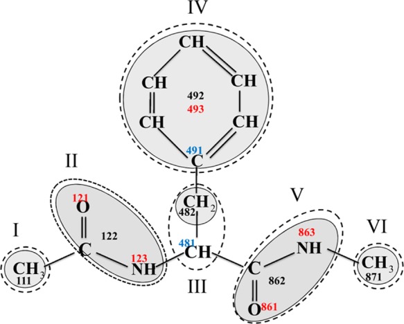
GBEMP mapping schemes for phenylalanine (Phe) dipeptides. Each rigid body, being enclosed by a dash line, consists of a Gay–Berne particle (represented by shadowed ellipsoid, sphere or disk) with a few electric multipoles or without any electric multipole. The indices of rigid bodies, Gay–Berne sites, interacting EMP sites and noninteraction EMP sites (just serve as connecting different rigid bodies), are indicated by Roman numbers and Arabic numbers in black, red, and blue, respectively.
In Figure 1, the GBEMP model of the phenylalanine dipeptide consists of six rigid bodies (I through VI) that are connected by virtual or valence bonds. Bonding occurs between two different rigid bodies through Gay–Berne or EMP sites. Each rigid body is composed of at least one Gay–Berne particle (ellipsoid, sphere, or disk) with or without EMP sites. The Gay–Berne sites 111, 482, 871 in the spherical rigid bodies (I, III and VI) corresponds to methyl groups (−CH2 or −CH3), the Gay–Berne sites 122 and 862 in the elliptical rigid bodies (II and V) are positioned at the centers of mass of corresponding peptide groups (−CONH-), and the Gay–Berne site 492 is located at the center of mass of disklike rigid body (IV) corresponding to the phenyl group (−C6H5); oxygen atoms of peptide groups are regarded as the positions of the EMP sites 121 and 861 included in the elliptical rigid bodies (II and V), and nitrogen atoms of peptide groups as the locations of the EMP sites 123 and 863 in the elliptical rigid bodies (II and V); the EMP site 493 shares the same spot with the Gay–Berne site 492 in the disklike rigid body (V); the EMP sites 481 and 491, located at α and γ carbon atoms respectively, are considered as the noninteraction sites serving the purpose to connect two different rigid bodies. In such that, bonds exist between sites (111,122), (123, 481), (482, 491), (481, 862), and (862, 871), one example of an angle consists of the sites (111, 122, 123) and that of a torsion angle is composed of the sites (111, 122, 123, 481). The nonbonded interactions between different Gay–Berne particles and between EMP sites in different rigid bodies are given in the following section.
GBEMP Energy Function
In GBEMP model, the effective energy function is a sum of different energy terms
| 1 |
where Ubond, Uangle, and Utorsion correspond to bond stretching, angle bending and torsional potentials, respectively. The bond stretching term adopts the fourth-order Taylor expansion of the Morse potential, the bond angle bending term utilizes a sixth-order potential, and a three-term Fourier series expansion is employed to calculate torsional energies. These valence potentials adopt similar functional forms being used by classical molecular mechanics potentials, such as MM350
| 2 |
| 3 |
| 4 |
The parameters for bond stretching, angle bending and torsional potentials were obtained through fitting to the potentials of mean force (PMFs) constructed by sampling atomic configurations from molecular dynamics simulations of dipeptides using CHARMM force field (with CMAP).51 Then, the parameters for torsional potentials were optimized in the CG MD simulations of dipeptides through iteratively matching to experimental results for the distributions of backbone torsion (ϕ/ψ) and side chain torsion χ1.
Gay–Berne Potential
The Gay–Berne anisotropic potential energy function UGB is given by the form
 |
5 |
The range parameter σ and the strength parameter ε for pairwise interactions are functions of the relative orientation of the Gay–Berne particles. Each uniaxial molecule is associated with a set of Gay–Berne parameters that describe its shape (ellipsoid, sphere, or disk) and the orientation of its principal axis in the inertial frame, defined according to the all-atom model. The term dw is used to control the “softness” of the potential.40 A generalized form of the range parameter σ(ûi, ûj, r̂ij) is described as
| 6 |
where
| 7 |
| 8 |
| 9 |
The notations l and d describe the length and breadth of Gay–Berne particles. The terms χα2, χα–2, and χ2 can be calculated as
| 10 |
| 11 |
| 12 |
The total well-depth parameter is computed as
| 13 |
The term ε0 refers to the well depth of the cross configuration; the orientation-dependent strength terms ε1 and ε2 are calculated in the following manner
| 14 |
| 15 |
where
| 16 |
| 17 |
The notation εE is the well depth of the end-to-end/face-to-face configuration, and εS is the well depth of the side-by-side configuration. Between unlike pairs, all values and their εS and εE are specified explicitly or computed using a combining rule employed in AMOEBA polarizable force field.52,53 The parameters μ and ν were set to canonical values of 2.0 and 1.0, respectively. The terms χ′2, χ′α′2, and χ′α′–2 were treated as inseparable and computed directly as:
| 18 |
| 19 |
| 20 |
The procedure of obtaining the parameters for the Gay–Berne energy term UGB is described in more details in the Results and Discussion.
Electric Multipole Potential
The interaction energy between two electric multipole sites can be expressed in its polytensor form:52
| 21 |
or in its expanded form
 |
22 |
where q, d, and Q are charge, dipole, and quadrupole moments, respectively. The point–multipole model can accurately describe the electrostatic interactions between CG particles being separated with a certain distance (>5 Å). When two CG particles are getting too close, however, the point-multipoles cannot correctly represent the actual overlap of their charge distributions such that the penetration error is produced. To avoid the spurious interaction energy when two CG particles interacting at very short-range (<5 Å), an effective solution to correct the penetration error would be to introduce a damping function,54 which was implemented to the multipole moments in each pair of interaction sites. The damping function in this work has the functional form
| 23 |
where u is the effective distance and defined by u = rij/(αiαj), in which rij represents the actual distance between particles i and j, and αi indicates the “size” of the particle i. The factor a is a dimensionless parameter to control the damping strength. In this model, the value of a was tentatively set to 0.49. The λ is applied to the regular formula of multipole interaction energy and forces and approaches unity as the distance rij increases. This method has proven to be effective in dealing with polarization catastrophe of point polarizable model.52 By introducing the damping function, the point multipoles are replaced by smeared charge distributions. As such, the penetration problem can be avoided. The parametrization of electric multipole potential UEMP is presented in more details in the Results and Discussion.
Molecular Dynamics Simulations of Dipeptides
To determine the GBEMP parameters for bond stretching, angle bending, and torsional potentials, we have carried out atomistic molecular dynamics simulation on amino acid dipeptides using the CHARMM22 force field with the CMAP torsion potential.51 Each dipeptide was blocked with an acetyl group (ACE) at the N terminus and with N-methylamide (NME) at the C terminus. Each system was solvated in explicit waters (at pH 7) in a cubic box with the distance of at least 12 Å from the surface of the dipeptide to the edge of the box. Each charged amino acid was neutralized with either chlorine or solium ion, which was randomly placed by replacing the overlapping water molecules. Initial configuration was briefly minimized and then heated up to from 100 to 300 K through a series of simulations. Then a 100 ps NPT simulation (equilibration run) under 300 K was followed by a NPT production run of at least 100 ns to generate the trajectory for final analysis. The periodic boundary condition was employed to avoid solvent boundary artifact. Electrostatic interactions were calculated with the particle-mesh Ewald method55 using a 32 × 32 × 32 grid for the discrete fast Fourier transform (FFT) and a direct space cutoff of 9 Å. During the simulation, SHAKE56 was applied to constrain the lengths of bonds involving hydrogen so that an integration time step of 2 fs could be used. The temperature was controlled using the Nose–Hoover algorithm.57
The coarse-grained (CG) MD simulation protocol used in this work is described as follows. For each dipeptide model, the CG MD simulation in generalized Kirkwood (GK) implicit solvent58 was carried out in the “GBEMP” suite based on TINKER program and the equation of motion was integrated using the Euler’s rigid body integrator46 with the integration step of 5 fs. The nonbonded interaction cutoff was set to 12 Å with the truncate scheme, and van Der Waals (vdW) interactions between 1 and 2 and 1 and 3 neighbors were scaled by 0.01 and 0.7, respectively. Each system was minimized and then was followed by an equilibration MD run of a few nanoseconds under the temperature of 300 K. To generate the trajectory for final analysis, at least 1 microsecond CG MD simulations were carried out on dipeptides while 20 ns CG MD simulations were performed on two proteins under the temperature of 300 K.
Results and Discussion
Parameterization of Gay–Berne Potential
To determine Gay–Berne parameters for the CG particles predefined in the phenylalanine dipeptide model (Figure 1), the atomistic energy profiles for the van der Waals (vdW) interactions between homodimers of CH4, HCONH2, and C6H6, each of which adopts different special configurations (such as, side-by-side, end-to-end/face-to-face, etc.) at various separations (from short to long distances), were constructed using AMOEBA all-atom model. At each separation, the homodimer interaction energy (Figure 2) was calculated as a Boltzmann average over conformations generated by rotating one molecule around its primary axis. In this work, the Gay–Berne particles for CH4, HCONH2, and C6H6 were treated as sphere, ellipsoid, and disk, respectively. By employing a genetic algorithm, we obtained the Gay–Berne parameters by fitting to the atomistic energy profiles in gas phase and were further refined in the CG simulations of dipeptides if necessary, and the final Gay–Berne parameters for CH4, HCONH2, and C6H6 are listed in Table 1.
Figure 2.

Atomistic energy profiles (dash lines) for the vdW interactions between homodimers of the (A) CH4, (C) HCONH2, and (E) C6H6 molecules, each of which adopts different special configurations at various separations, were constructed using AMOEBA all-atom model. The solid lines represent Gay–Berne interaction energies. Meanwhile, the correlations between the Gay–Berne and AMOEBA results for the vdW interactions between homodimers of (B) CH4, (D) HCONH2, and (F) C6H6, were measured in this work, respectively.
Table 1. Gay–Berne Parameters of the Coarse-Grained Particles Defined in the Phenylalanine Dipeptide Model.
| index of Gay–Berne site | L (Å) | D (Å) | dw | ε0 (kcal/mol) | εE (kcal/mol) | εS (kcal/mol) |
|---|---|---|---|---|---|---|
| 111 | 2.475 | 2.475 | 1.000 | 0.343 | 1.000 | 1.000 |
| 122 | 3.763 | 2.462 | 1.202 | 0.681 | 1.479 | 1.437 |
| 482 | 2.475 | 2.475 | 1.000 | 0.343 | 1.000 | 1.000 |
| 492 | 2.475 | 2.475 | 1.000 | 0.343 | 1.000 | 1.000 |
| 862 | 3.763 | 2.462 | 1.202 | 0.681 | 1.479 | 1.437 |
| 871 | 2.475 | 2.475 | 1.000 | 0.343 | 1.000 | 1.000 |
To determine the Gay–Berne parameters of the coarse-grained particles included in the rigid bodies I and VI of phenylalanine dipeptide model, one needs to construct the atomistic energy profile for the vdW interactions between the CH4 homodimer. As the shape of the CH4 molecule was considered to be spherical in this work, the Gay–Berne potential, describing the vdW interactions between the two spherical particles, is equivalent to the well-known Lennard-Jones potential. Finally, the Gay–Berne parameters of the coarse-grained particles were determined from the match between Gay–Berne and AMOEBA results, as shown in Figure 2A. In the case of the HCONH2 molecule, the corresponding coarse-grained particle was considered as an ellipsoid, three special configurations (cross, end-to-end, and t-shape) of the HCONH2 homodimer were used to acquire the Gay–Berne parameters of the coarse-grained particles defined in the rigid bodies II and V of phenylalanine dipeptide model. As illustrated in Figure 2B, the comparison between Gay–Berne and AMOEBA results can reveal the quality of the obtained Gay–Berne parameters. In the case of the C6H6 molecule, the shape of the molecule was regarded to be disklike; thereby, three special configurations (face-to-face, side-by-side and t-shape) of the C6H6 homodimer were used for the calculation of the vdW intermolecular interactions at different separations. By fitting to the atomistic energy profile (see Figure 2C), the Gay–Berne parameters were obtained for the Gay–Berne particle in the rigid body IV of the phenylalanine dipeptide model. Meanwhile, the correlations between Gay–Berne and AMOEBA results for the vdW interaction energies of these homodimers were evaluated as given in Figure 2B, 2D, and 2F respectively, indicating the quality of the Gay–Berne parameters.
Similarly, for the other amino acid models, the Gay–Berne parameters of the CG particles defined in Supporting Information Figure S2 were obtained through fitting to the AMOEBA atomistic interaction energy profiles of corresponding all-atom models and were further refined in the following CG simulations of dipeptides. The final Gay–Berne parameters of the CG particles for all amino acids are given in Supporting Information Table S1.
Parameterization of Electric Multipole Potential
In the GBEMP model of phenylalanine dipeptide, one EMP site was included in the rigid body III and two EMP sites were placed in the rigid bodies II, IV, and V, respectively. Among these EMP sites, one should note that the sites 481 and 491 are noninteraction EMP sites, which just serve as the purpose of connecting two different rigid bodies. Thus, to obtain the EMP parameters of phenylalanine dipeptide model, one only needs to determine the EMP parameters of the coarse-grained particles of the corresponding HCONH2 and C6H6 molecules. Note that AMOEBA atomic multipole moments for atoms were calculated from the ab initio quantum mechanics using Stone’s distributed multipole analysis,59 so it is quite straightforward to expand the point multipoles at any location in HCONH2 and C6H6. In this work, the point multipoles were placed at oxygen and nitrogen atoms for the HCONH2 molecule, and at the center of mass of corresponding atoms for the C6H6 molecule. To optimize the EMP parameters of the coarse-grained particles (HCONH2 and C6H6), we have constructed the AMOEBA atomistic energy profiles for the electrostatic interactions between HCONH2 and H2O, and between the C6H6 homodimer, respectively, as given in Figure 3. The correlations between EMP and AMOEBA electrostatic interaction energies were measured as shown in Figure 3B and 3D, showing good agreement between two models. The final optimized EMP parameters for the phenylalanine dipeptide model are listed in Table 2. In the same way, the EMP parameters for the other amino acid models were derived from the QM calculations based on the Stone’s distributed multipole analysis and were further refined in the calculations of electrostatic interactions between homodimers and/or between heterodimers, and all EMP parameters are given in Supporting Information Table S2.
Figure 3.

Atomistic energy profiles (dash lines) for the electrostatic interactions (A) between HCONH2 and H2O and (C) between C6H6 homodimer, have been constructed using AMOEBA all-atom model. The solid lines represent the coarse-grained EMP energy profiles. Meanwhile, the correlations between the coarse-grained and AMOEBA models for two systems (HCONH2–H2O and C6H6–C6H6) were measured and given in panels B and D, respectively.
Table 2. EMP Parameters of the Coarse-Grained Particles Defined in the Phenylalanine Dipeptide Model.
| index of EMP site | charge | dipole | quadrupole | ||
|---|---|---|---|---|---|
| 121 | 0.000 | –1.463 | 2.001 | –1.148 | –0.014 |
| 0.281 | –1.148 | –0.927 | 0.009 | ||
| –0.003 | –0.014 | 0.009 | –1.074 | ||
| 123 | 0.000 | 0.879 | 1.067 | –1.148 | 0.138 |
| –0.437 | –1.148 | 1.258 | –0.128 | ||
| –0.024 | 0.138 | –0.128 | –2.325 | ||
| 493 | 0.000 | 0.879 | 1.067 | –1.148 | 0.138 |
| –0.437 | –1.148 | 1.258 | –0.128 | ||
| –0.024 | 0.138 | –0.128 | –2.325 | ||
| 861 | 0.000 | –1.463 | 2.001 | –1.148 | –0.014 |
| 0.281 | –1.148 | –0.927 | 0.009 | ||
| –0.003 | –0.014 | 0.009 | –1.074 | ||
| 863 | 0.000 | 0.879 | 1.067 | –1.148 | 0.138 |
| –0.437 | –1.148 | 1.258 | –0.128 | ||
| –0.024 | 0.138 | –0.128 | –2.325 | ||
The quality of the optimized EMP parameters for different dipeptide models have been further evaluated by calculating their dipole moments using both GBEMP and AMOEBA models. The correlations between the two models for the magnitude of dipeptide dipole moment and x, y, and z components have been calculated respectively, as shown in Figure 4 and Supporting Information Figure S2, demonstrating good quality of the GBEMP model, especially for hydrophobic amino acid residues. In the calculations of the dipole moment for each dipeptide, the atomistic configurations were chosen randomly from the structures generated from atomistic MD simulations (using AMOEBA force field), and the correlations did not vary significantly by randomly selecting different sets of conformations. Furthermore, for each dipeptide model, a number of waters were generated randomly surrounding it (any heavy atom in a dipeptide molecule was separated from an oxygen atom of the water molecule in the range of 3.0–5.0 Å), and then the electrostatic interaction energies were calculated between the dipeptide and a single water being placed at different positions, showing rather encouraging agreement between GBEMP and AMOEBA models, as seen in Figure 5.
Figure 4.


Correlations between the GBEMP and AMOEBA results for the magnitude of the dipole moment of different dipeptide models (20 kinds of dipeptides in total). In the calculations of the dipole moment for each dipeptide model, various conformations were chosen randomly from the atomistic structures generated from atomistic MD simulation (using AMOEBA force field).
Figure 5.


Correlations between GBEMP and AMOEBA results for electrostatic interactions between dipeptides and a single water (each water was placed in different positions, see insert figures). For each dipeptide (its atomistic representation is shown in colored sticks in each inset figure respectively), a number of waters (only oxygen atoms are shown in red beads in inset figures) were generated randomly surrounding it (any heavy atom in a dipeptide molecule was separated from an oxygen atom of any generated water molecule in the range of 3.0–5. 0 Å), and then the electrostatic interaction energies were calculated between the dipeptide and a single water placed in different positions respectively.
Intermolecular Interactions between Dipeptides
The performance of the GBEMP model for amino acid dipeptides was further examined by comparing the GBEMP and atomistic results for the intermolecular interaction energies between dipeptide homodimers and heterodimers. In this work, we have constructed twenty dipeptide homodimers (such as Ala/Ala, Arg/Arg, ..., Val/Val), and the intermolecular interaction energies of each system were calculated at different separations by using AMOEBA atomistic and GBEMP coarse-grained force fields respectively. In addition, three specific dipeptide heterodimers, such as Gln/Glu, Gln/Lys, and Glu/Lys, were chosen for the study because they represent the intermolecular interactions between neutral and charged amino acids, and between charged amino acids respectively. The comparison between GBEMP and AMOEBA results for a few representative intermolecular interactions are given in Figure 6, and van der Waals, electrostatic and total interaction energies for all dipeptide dimers are presented in left, middle and right columns of Supporting Information Figure S3, respectively, showing the promising future of the GBEMP model in the study of intermolecular interactions between dipeptide dimers.
Figure 6.

Intermolecular interaction energies for peptide dimers: (A) Phe/Phe, (B) Glu/Glu, (C) Gln/Gln, (D) Gln/Glu, (E) Gln/Lys, and (F) Lys/Lys, using AMOEBA atomistic force field (in black) and GBEMP coarse-grained force field (in red).
From Supporting Information Figure S3, it can be observed that, comparing to atomistic AMOEBA model, the GBEMP model slightly underestimated the van der Waals interaction energies in the attractive region. The worse case was found in the calculation of the vdW interaction energies for the Asp homodimer, showing the difference of 2.5 kcal/mol between two models at the deepest point of the potential well (Supporting Information Figure S3). The difference of less than 1.0 kcal/mol between two models, however, was observed for most of cases, indicating that the current Gay–Berne parameters for dipeptide models are satisfactory.
The electrostatic interaction energies for dipeptide dimers have been compared between the AMOEBA and GBEMP models in Supporting Information Figure S3. Particularly, we have shown that our GBEMP model was able to correctly capture the repulsive feature of the electrostatic interactions for some dipeptide dimers, such as Arg/Arg, Asp/Asp, Glu/Glu, Gly/Gly, Gln/Glu, Lys/Lys, and Pro/Pro, as well as the attractive property of the electrostatic interactions for some other dipeptide dimers, such as Ala/Ala, Asn/Asn, Cys/Cys, Gln/Gln, Ile/Ile, Leu/Leu, Met/Met, Phe/Phe, Ser/Ser, Thr/Thr, Trp/Trp, Tyr/Tyr, Val/Val, Gln/Lys, and Lys/Glu.
In summary, the outstanding agreement between the GBEMP and AMOEBA models in the calculations of intermolecular interactions between dipeptide homodimers or between dipeptide heterodimers, including the electrostatic and vdW components, should lie on the anisotropic nature of the Gay–Berne potential as well as the explicit treatment of electric multipole potential. To further improve the transferability of the GBEMP model, it appears to be more reasonable if dipeptide dimers adopting more different configurations are chosen as the training sets to optimize force field parameters. However, it is impractical to comply with this idea because of computational expenses or insufficient sampling. It is believable that the best way of increasing the quality of GBEMP protein model should be to use a large training set of proteins from protein data bank for the parametrization, which is ongoing work.
Distribution of the Backbone Torsions (ϕ/ψ)
Under a physiological condition, a folded protein usually consists of α-helical and β-strand secondary structure elements connected by random coils, such as turns and loops. It has been recognized that both protein structure and conformational dynamics are essential to biology function. Therefore, to thoroughly understand protein functions, it is necessary to obtain dynamic information of secondary structure elements, which are related to two degrees of freedom: the backbone torsion angles ϕ(C–N–Ca–C) and ψ(N–Ca–C–N). For instance, the Ramachandran plot,60 describing the (ϕ/ψ) distribution, has been extensively used to illustrate the propensity of the formation of secondary structures for amino acids. In general case (except for glycine and proline), the well-known Ramachandran plot gives two major minima: (1) the first one is located in the neighborhood of αR (ϕ ≈ −60, ψ ≈ −40) which belongs to α basin; (2) the second one is observed in the region PPII (ϕ ≈ −60, ψ ≈ 150) or C5 (ϕ ≈ −150, ψ ≈ 170) of β basin. In addition, some minor minima having higher relative free energies are observed at αL (ϕ ≈ 60, ψ ≈ 40) and C7ax (ϕ ≈ −75, ψ ≈ 75), which are believed to be relevant to the formation of turns and loops. However, the conformational preferences of proline (Pro) are restricted to two regions αR (ϕ ≈ −60, ψ ≈ −40) and PPII (ϕ ≈ −60, ψ ≈ 150). In contrast, glycine (Gly) has more conformational preferences distributed in many different regions.
From the data gathered from Dunbrack Library,61 (see Figure 7), it appears that, in the β basin, alanine (Ala), arginine (Arg), cysteine (Cys), glutamine (Gln), glutamic acid (Glu), histidine (His), leucine (Leu), lysine (Lys), methionine (Met), phenylalanine (Phe), serine (Ser), threonine (Thr), and tyrosine (Tyr) follow a similar energy pattern that two minima are separated by a very shallow barrier. From the GBEMP results (Figure 8), two minima were also found in the β basin for arginine (Arg), glutamic acid (Glu), phenylalanine (Phe), serine (Ser), threonine (Thr), and tyrosine (Tyr), but only one minimum was observed for alanine (Ala), cysteine (Cys), glutamine (Gln), histidine (His), leucine (Leu), lysine (Lys), and methionine (Met). However, the relative populations of the β region for these amino acids are matched reasonably well between the GBEMP model and experimental results, see Table 3.
Figure 7.

Potential of mean force (PMF) results for the backbone torsion (ϕ/ψ) distributions of amino acids, calculated from the experimental protein structures (Dunbrack Library). The color bars represent the free energy in the unit of kcal/mol.
Figure 8.

Potential of mean force (PMF) results for the backbone torsion (ϕ/ψ) distributions of amino acids, calculated from the GBEMP simulations of dipeptides. The color bars represent the free energy in the unit of kcal/mol.
Table 3. Relative Populations of Different Regions (αR, β and αL) in the (ϕ/ψ) Distribution for Amino Acids Obtained from the Experimental Protein Structures (Dunbrack Library) and GBEMP Simulations of Dipeptides.
| αR |
β |
αL |
||||
|---|---|---|---|---|---|---|
| amino acid | experiment | GBEMP | experiment | GBEMP | experiment | GBEMP |
| Ala | 0.463 | 0.464 | 0.450 | 0.447 | 0.040 | 0.033 |
| Arg | 0.568 | 0.654 | 0.389 | 0.271 | 0.022 | 0.049 |
| Asn | 0.471 | 0.587 | 0.362 | 0.269 | 0.097 | 0.101 |
| Asp | 0.522 | 0.651 | 0.366 | 0.296 | 0.044 | 0.034 |
| Cys | 0.601 | 0.577 | 0.356 | 0.412 | 0.026 | 0.000 |
| Gln | 0.601 | 0.588 | 0.356 | 0.325 | 0.026 | 0.050 |
| Glu | 0.644 | 0.639 | 0.324 | 0.326 | 0.018 | 0.022 |
| His | 0.476 | 0.617 | 0.454 | 0.382 | 0.033 | 0.000 |
| Ile | 0.429 | 0.380 | 0.564 | 0.619 | 0.001 | 0.000 |
| Leu | 0.567 | 0.570 | 0.413 | 0.388 | 0.007 | 0.014 |
| Lys | 0.581 | 0.589 | 0.373 | 0.410 | 0.029 | 0.000 |
| Met | 0.560 | 0.715 | 0.408 | 0.284 | 0.013 | 0.000 |
| Phe | 0.450 | 0.475 | 0.512 | 0.478 | 0.015 | 0.046 |
| Ser | 0.468 | 0.462 | 0.484 | 0.503 | 0.016 | 0.000 |
| Thr | 0.455 | 0.485 | 0.512 | 0.501 | 0.003 | 0.010 |
| Trp | 0.489 | 0.589 | 0.475 | 0.368 | 0.012 | 0.004 |
| Tyr | 0.452 | 0.563 | 0.506 | 0.432 | 0.016 | 0.000 |
| Val | 0.378 | 0.355 | 0.614 | 0.618 | 0.001 | 0.013 |
The experimental free energy maps for the hydrophobic residues, isoleucine (Ile) and valine (Val), exhibit a single minimum in the β basin that is close to the C7eq region. This feature has been captured by our GBEMP result for valine (Val). It is surprising that two minima were observed from the GBEMP energy map but one single minimum was found in the experimental free energy map. The difference may be ascribed to the reason that the GBEMP results were obtained from simulating dipeptides while the experimental results were actually derived from the folded protein structures. In fact, the similar results have been observed from both the earlier work done by Feig62 and our current work by performing the atomistic simulation of valine (Val) using CHARMM force field (Supporting Information Figure S4).
Comparing to some other amino acids, aspartic acid (Asp) and asparagines (Asn) have overall broader β basin that includes the C7eq region. Although the GBEMP model for Asp and Asn have failed to reproduce this feature, the relative populations of the β region in the (ϕ/ψ) distribution are comparable between the GBEMP model and experimental results, see Table 3.
In the α basin, the experimental energy landscape based on the folded protein structures (Dunbrack Library) displays that the predominated conformations around the αR region have been sampled for all amino acids (Figure 7), which were observed in GBEMP results as well (Figure 8). In addition, the relative populations of the αR region are matched reasonably well between the two methods, see Table 3.
According to the experimental Ramachandran plot based on the Dunbrack library, most of amino acids have a shallow minimum in the αL basin, which are also captured by our GBEMP model in some cases. However, comparing to the β and αR basins, αL conformations are less populated, which have been correctly shown by our GBEMP model, explaining the excellent correlation between the experimental and GBEMP results in the (ϕ, ψ) distribution, see Figure 9.
Figure 9.

Correlation between the GBEMP and experimental (Dunbrack Library) results for the relative population of the three regions (αR, β, and αL) based on the Ramachandran plot for non-proline and non-glycine amino acids.
Distribution of the Side Chain Torsion χ1
According to the distribution of the side chain torsion χ1 for amino acids (except for Gly, Ala, and Pro residues) calculated from either experimental protein structures (Dunbrack Library) or our GBEMP simulations of dipeptides (see Figure 10), three dominated conformations were sampled in three narrow regions g– (∼ 60°), t (∼180°), and g+ (∼300°), and in general the relative population of the three regions follows the order of preference: g+ > t > g–, demonstrating the excellent correlation between the experimental and GBEMP results, as seen in Figure 11.
Figure 10.

Distributions of the side chain torsion χ1for amino acids (except for Gly, Ala, and Pro), calculated from the experimental protein structures (Dunbrack Library) and GBEMP simulations of dipeptides. Experimental and GBEMP results are represented by the dash and solid lines, respectively.
Figure 11.

Correlation between the GBEMP coarse-grained and experimental (Dunbrack Library) results for the relative population of the three regions (g–, t, and g+) in the χ1distribution for amino acids (except for Gly, Ala, and Pro).
In cases of the amino acids having the nonpolar or aromatic side chains, such as isoleucine (Ile), (leucine) Leu, (methionine) Met, valine (Val), phenylalanine (Phe), tryptophan (Trp) and tyrosine (Tyr), the slight difference between the GBEMP and experimental results for the χ1 distribution was observed. In particular, the excellent agreement between the GBEMP and experimental results was found in the most dominated region g+, where the relative population has been measured as of 0.51–0.81, see Table 4.
Table 4. Relative Populations of Different Regions (g–, t, and g+) in the χ1 Distribution for Amino Acids Obtained from the Experimental Protein Structures (Dunbrack Library) and GBEMP Simulations of Dipeptides.
|
g– |
t |
g+ |
||||
|---|---|---|---|---|---|---|
| amino acid | experiment | GBEMP | experiment | GBEMP | experiment | GBEMP |
| Arg | 0.087 | 0.177 | 0.338 | 0.329 | 0.575 | 0.494 |
| Asn | 0.148 | 0.099 | 0.299 | 0.294 | 0.553 | 0.607 |
| Asp | 0.164 | 0.087 | 0.332 | 0.357 | 0.504 | 0.556 |
| Cys | 0.171 | 0.231 | 0.264 | 0.302 | 0.565 | 0.467 |
| Gln | 0.071 | 0.061 | 0.312 | 0.395 | 0.617 | 0.544 |
| Glu | 0.080 | 0.246 | 0.336 | 0.250 | 0.584 | 0.504 |
| His | 0.125 | 0.093 | 0.350 | 0.254 | 0.524 | 0.652 |
| Ile | 0.123 | 0.057 | 0.086 | 0.135 | 0.791 | 0.807 |
| Leu | 0.013 | 0.082 | 0.332 | 0.215 | 0.655 | 0.703 |
| Lys | 0.069 | 0.056 | 0.344 | 0.453 | 0.587 | 0.490 |
| Met | 0.070 | 0.163 | 0.291 | 0.190 | 0.638 | 0.647 |
| Phe | 0.118 | 0.057 | 0.341 | 0.426 | 0.541 | 0.517 |
| Ser | 0.463 | 0.615 | 0.243 | 0.165 | 0.294 | 0.220 |
| Thr | 0.468 | 0.529 | 0.078 | 0.143 | 0.454 | 0.328 |
| Trp | 0.156 | 0.154 | 0.340 | 0.342 | 0.504 | 0.504 |
| Tyr | 0.123 | 0.203 | 0.346 | 0.317 | 0.531 | 0.480 |
| Val | 0.093 | 0.171 | 0.333 | 0.210 | 0.574 | 0.619 |
Among the amino acids with polar and uncharged side chains, asparagine (Asn), cysteine (Cys), and glutamine (Gln) still favor the g+ conformation, for instance, the relative populations of the three regions (g+, t, and g–) have been measured as of 0.55–0.62, 0.26–0.31 and 0.07–0.14, respectively, according to the experimental χ1 distribution (Dunbrack Library). However, in cases of serine (Ser) and threonine (Thr), the most dominated region switches to the g– conformation, the experimental relative population of which has been measured as of 0.46–0.47. It is exciting that these features observed from the experiment have been captured quite well by our GBEMP model, as shown in Table 4 and Figure 10. The obvious difference between the GBEMP and experimental results for serine (Ser) has been observed in the t region, perhaps owing to the different sampling methods adopted by experiment and theoretical modeling, as we mentioned above. For instance, this difference was similarly observed in the atomistic CHARMM simulation of serine dipeptide (see Supporting Information Figure S5).
As for the charged amino acids, such as arginine (Arg), aspartic acid (Asp), Glu, and lysine (Lys), their relative populations in the χ1 distribution have been measured as of 0.50–0.56, 0.33–0.34, and 0.07–0.16 for the g+, t, and g– regions, respectively, on the basis of the Dunbrack library. Generally speaking, our GBEMP model was able to capture main features observed from the experimental results, especially in cases of charged amino acids with long side chain, such as Arg, Glu, and Lys. Although the apparent difference in the χ1 distribution between experimental and GBEMP methods was observed for the charged amino acid having short side chain, such as Asp, the overall correlation between GBEMP and experimental results can be satisfactorily achieved in the χ1 distribution. As a matter of fact, the visible difference in the χ1 distribution has also been detected between atomistic and experimental results when the atomistic simulation of Asp dipeptide was performed by using CHARMM 27 force field with CMAP (Supporting Information Figure S5). The sampling method employed in theoretical and experimental models might contribute to the difference, as it happened in the case of serine (Ser).
Molecular Dynamics Simulations of Proteins
In this work, we attempt to apply the GBEMP model to study the dynamics of two test cases of proteins (PDB IDs 2M6O and 2LXY),63,64 which have different secondary structures and sizes. Actinobacterial transcription factor RdpA (PDB ID 2M6O)63 is a small protein (48 amino acid residues) consisting of two antiparallel β-sheets; 2-mercaptophenol-α3C (PDB ID 2LXY)64 is a three α helix-bundle protein of 67 amino acid residues. In order to evaluate the quality of our GBEMP model in modeling the proteins, we have also carried out atomistic MD simulations on the two cases using AMBER 03 force field65 in the AMBER simulation package.66
The backbone Cα root-mean-square deviations (RMSDs) of two proteins, plotted in Figures 12A and 13A, were measured as of around 4.0 Å, indicating that the overall native structures of the proteins were reasonably maintained throughout the coarse-grained MD simulations. Figures 12A and 13A show that the coarse-grained MD simulations reached equilibrium within 10 ns while the equilibrium can be obtained within 2 ns as for the atomistic MD simulations. So, the last 10 and 3 ns were considered as the production runs for the coarse-grained and atomistic MD simulations respectively. Although larger RMSD values were observed for the GBEMP model when comparing to atomistic AMBER model, the difference of the equilibrated RMSD values between the GBEMP and atomistic AMBER models is about 1.5 Å, acceptable for a coarse-grained model.
Figure 12.
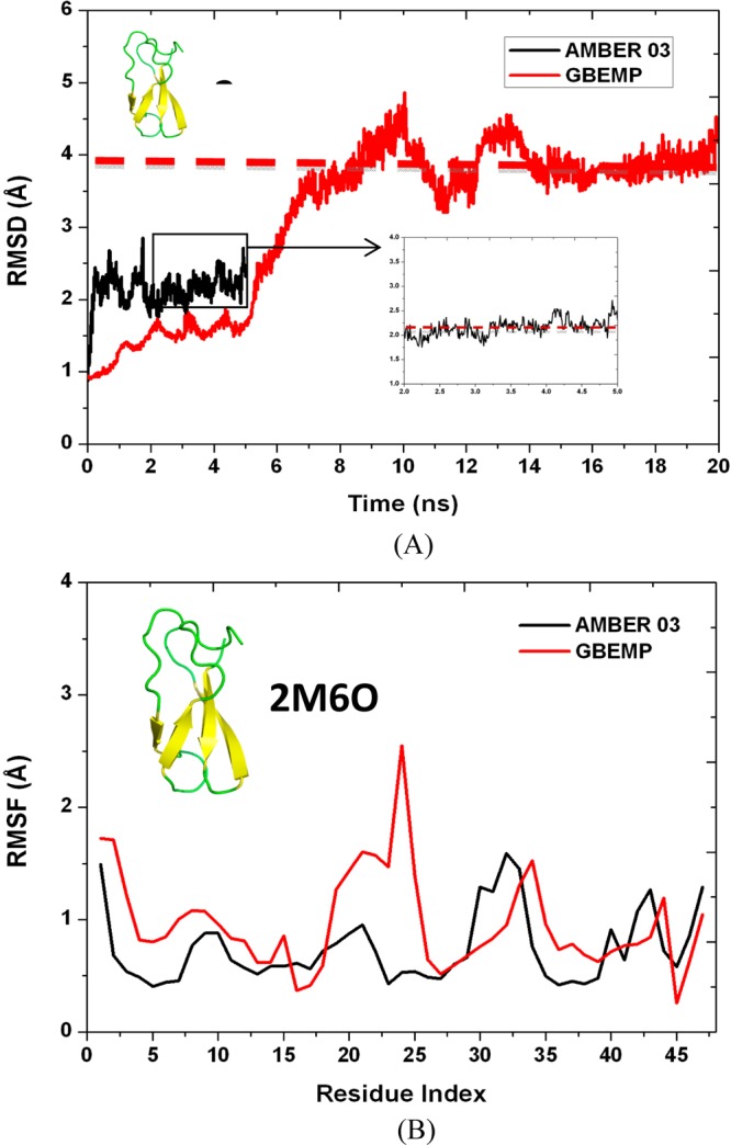
(A) RMSD values of the backbone Cα atoms from the crystal structure (PDB ID 2M6O) and (B) RMSF values of the backbone Cα atoms were calculated using AMBER 03 atomistic force field (in black) and GBEMP coarse-grained force field (in red).
Figure 13.

(A) RMSD values of the backbone Cα atoms from the crystal structure (PDB ID 2LXY) and (B) RMSF values of the backbone Cα atoms were calculated using AMBER 03 atomistic force field (in black) and GBEMP coarse-grained force field (in red).
The backbone Cα root-mean-square fluctuations (RMSFs) along amino acid sequence of a protein can provide the information about the protein’s flexibility. The peaks indicate the high flexibility while the valleys are associated with the low flexibility. In the case of the actinobacterial transcription factor RdpA, the overall RMSF landscape of the atomistic AMBER model is consistent with that of our GBEMP model (Figure 12B), especially in the regions near either N-terminus or C-terminus. The RMSF values in the region (residues 20–25) were overestimated by GBEMP model; however, the segment (residues 20–25) belongs to an intrinsically flexible loop connecting two antiparallel beta sheets. In the case of 2-Mercaptophenol-alpha3C protein, the atomistic model has shown that the two regions (residues 22–26 and residues 44–48) are significantly flexible, and this feature was captured by the GBEMP model (Figure 13B). Overall the peaks and valleys in the atomistic RMSF landscape were reasonably well reproduced by the coarse-grained model, demonstrating that this anisotropic model is promising in modeling proteins.
In the end, we would like to point out that the computational efficiency of our GBEMP model is upbeat in modeling proteins. When we simulated the protein 2M6O (48 residues) by using coarse-grained GBEMP and atomistic AMBER models with a single processor, a day was needed for the GBEMP simulation to acquire the 20 ns MD trajectory while it was necessary to spend about 13 days to obtain the 5 ns atomistic MD trajectory. Similarly, in the case of the protein 2LXY (67 residues), 2.5 days was required for the 20 ns GBEMP simulation and a month for the 5 ns AMBER simulation with TIP3P waters. Therefore, in both cases, the GBEMP model would be able to speed up MD simulation by the factor of around 50 with acceptable loss of accuracy. In this respect, our GBEMP model can outperform the PRIMO CG model, which has been tested with achieving about 10 to 20 speedup compared to CHARMM atomistic simulation in an explicit solvent. Although our GBEMP model underperforms the MARTINI coarse-grained model (achieving about 75–100 speedup)67 in terms of speed, it is believable that our GBEMP model would be more accurate than the MARTINI model due to the use of anisotropic Gay–Berne potential and the inclusion of electric multipoles. Furthermore, by comparing the speed of GBEMP model with that of AMOEBA and CHARMM models in simulating dipeptides in implicit solvents (GK model for AMOEBA and GB model for CHARMM), the speedup factor of about 50–200 can be achieved compared to implicit AMOEBA simulations and that of about 10–50 can be reached compared to implicit CHARMM simulations respectively, depending on the type of amino acids. This speed-up will be further improved by optimizing the preliminary rigid-body MD code.
Conclusions
In most of coarse-grained models, the coarse-grained particles are considered to be isotropic. However, in a biomolecular system, a coarse-grained particle, representing a group of atoms, is actually anisotropic, and thus it is necessary to use anisotropic potentials to provide accurate description of the nonbonded interactions. Among a variety of anisotropic potentials, the Gay–Berne potential, based on a Gaussian-overlap potential, has been extensively used to measure the van der Waals interactions between the coarse-grained particles being considered to be elliptic. In this paper, we presented the extension of the GBEMP coarse-grained model, adopting the framework of combining anisotropic Gay–Berne potential with point electric multipole (EMP) potential, to accurately and efficiently model amino acid dipeptides and proteins. In the GBEMP model, the atomistic information of amino acids was well preserved in the rigid bodies composed of Gay–Berne particles and point electric multipoles. Thus, the GBEMP model can not only be used to study proteins in a standalone fashion but can also be combine with other atomistic models in the “parallel” or “serial” manner.
The GBEMP model was parametrized to reproduce the individual energy components, vdW, and electrostatics, of the atomistic force field. As for various peptide–peptide and peptide–water systems, the coarse-grained model was able to provide the description of nonbonded interactions comparable to atomistic AMOEBA model. Furthermore, for each dipeptide model, the excellent correlation between GBEMP and AMOEBA models was observed in the calculations of the dipole moment (total magnitude, x-, y-, and z-components), providing additional support for the promising performance of the GBEMP model
For a variety of common amino acids, the conformational distributions of the backbone torsional angles (ϕ, ψ) and the side chain torsion χ1 were both in excellent agreement with PDB structural statistics (Dunbrack Library). In addition, two proteins (2M6O and 2LXY) having different sizes and structures were simulated to evaluate the quality of the GBEMP model. It has been shown that the native structures of the proteins were reasonably maintained and the landscape of B-factors derived from atomistic simulations was mostly reconstructed by the GBEMP model. Meanwhile comparing to AMOEBA, AMBER and CHARMM force fields, the computational cost of the GBEMP model in simulating proteins can be reduced about 10–200 times, depending on specific cases or atomistic models.
Acknowledgments
This work is supported by grants from the Ministry of Science and Technology of China (863 project No. 2012AA01A305; 973 project No. 2012CB721002), and the National Science Foundation of China under Contract No. 31370714, 91227126). “Hundreds Talent Program” of Chinese Academy of Sciences. P.R. acknowledges support by Welch foundation (F-1691) and National Institute of Health (GM106137).
Supporting Information Available
Gay–Berne and EMP parameters for the coarse-grained particles defined in dipeptide models (as shown in Figure S1), the correlations between the GBEMP and AMOEBA results for the calculations of x-, y-, z-components of the dipole moment of different dipeptide models, the comparison between the GBEMP and AMOEBA results for intermolecular interaction energies of dipeptide homodimers and heterodimers, the potentials of mean force (PMFs) for the (ϕ/ψ) distribution for valine (Val), calculated from the GBEMP and CHARMM simulations, and the distributions of the side chain torsion χ1 for serine (Ser) and aspartic acid (Asp) from the experimental protein structures (Dunbrack Library) and CHARMM atomistic simulations of dipeptides. This material is available free of charge via the Internet at http://pubs.acs.org.
Author Contributions
GH Li designed the study. GH Li, H.S., and Y.L. performed the research. GH Li, P.R., H.S. and Y.L. analyzed the data. GH Li and H.S. wrote the manuscript with comments from P.R.. H.S. and Y.L. contributed equally to this work.
The authors declare no competing financial interest.
Funding Statement
National Institutes of Health, United States
Supplementary Material
References
- Sherwood P.; Brookes B. R.; Sansom M. S. P. Curr. Opin. Struct. Biol. 2008, 18, 630–640. [DOI] [PMC free article] [PubMed] [Google Scholar]
- Tozzini V. Acc. Chem. Res. 2010, 43, 220–230. [DOI] [PubMed] [Google Scholar]
- Merchant B. A.; Madura J. D. Annu. Rep. Comput. Chem. 2011, 7, 67–85. [Google Scholar]
- Shen H.; Xia Z.; Li G.; Ren P. Annu. Rep. Comput. Chem. 2012, 8, 129–148. [Google Scholar]
- Ayton G. S.; Voth G. A. Curr. Opin. Struct. Biol. 2009, 19, 138–144. [DOI] [PMC free article] [PubMed] [Google Scholar]
- Karzbrun E.; Shin J.; Bar-Ziz R. H.; Noireaux V. Phys. Rev. Lett. 2011, 106, 048104. [DOI] [PubMed] [Google Scholar]
- Clementi C. Curr. Opin. Struct. Biol. 2008, 18, 10–15. [DOI] [PubMed] [Google Scholar]
- Wohlert J.; Berglund L. A. J. Chem. Theory Comput. 2011, 7, 753–760. [Google Scholar]
- Scott K. A.; Bond P. J.; Ivetac A.; Chetwynd A. P.; Khalid S.; Sansom M. S. P. Structure 2008, 16, 621–630. [DOI] [PubMed] [Google Scholar]
- Liwo A.; Khalili M.; Scheraga H. A. Proc. Natl. Acad. Sci., U.S.A. 2005, 102, 2362–2367. [DOI] [PMC free article] [PubMed] [Google Scholar]
- Wu C.; Shea J. E. Curr. Opin. Struct. Biol. 2011, 21, 209–220. [DOI] [PubMed] [Google Scholar]
- Arkhipov A.; Freddolino P. L.; Schulten K. Structure 2006, 14, 1767–1777. [DOI] [PubMed] [Google Scholar]
- Martinetz T.; Schulten K. Neural Networks 1994, 7, 507–522. [Google Scholar]
- Tirion M. Phys. Rev. Lett. 1996, 77, 1905–1908. [DOI] [PubMed] [Google Scholar]
- Haliloglu T.; Bahar I.; Erman B. Phys. Rev. Lett. 1997, 79, 3090–3093. [Google Scholar]
- Buchete N. V.; Straub J. E.; Thirumalai D. Curr. Opin. Struct. Biol. 2004, 14, 225–232. [DOI] [PubMed] [Google Scholar]
- Lazaridis T.; Karplus M. Curr. Opin. Struct. Biol. 2000, 10, 139–145. [DOI] [PubMed] [Google Scholar]
- Skolnick J. Curr. Opin. Struct. Biol. 2006, 16, 166–171. [DOI] [PubMed] [Google Scholar]
- Moult J. Curr. Opin. Struct. Biol. 1997, 7, 194–199. [DOI] [PubMed] [Google Scholar]
- Betancourt M. R. Proteins 2009, 76, 72–85. [DOI] [PubMed] [Google Scholar]
- Dehouck Y.; Gilis D.; Rooman M. J. Biophys. J. 2006, 90, 4010–4017. [DOI] [PMC free article] [PubMed] [Google Scholar]
- Ben-Naim A. J. Chem. Phys. 1997, 107, 3698–3706. [Google Scholar]
- Thomas P. D.; Dill K. A. J. Mol. Biol. 1996, 257, 457–469. [DOI] [PubMed] [Google Scholar]
- Mullinax J. W.; Noid W. G. Proc. Natl. Acad. Sci. U.S.A. 2010, 107, 19867–19872. [DOI] [PMC free article] [PubMed] [Google Scholar]
- Levitt M.; Warshel A. Nature 1975, 235, 694–698. [DOI] [PubMed] [Google Scholar]
- Trylska J.; Tozzini V.; Chang C. E.; McCammon J. A. Biophys. J. 2007, 92, 4179–4187. [DOI] [PMC free article] [PubMed] [Google Scholar]
- Tozzini V.; Trylska J.; Chang C. E.; McCammon J. A. J. Struct Biol. 2007, 157, 606–615. [DOI] [PubMed] [Google Scholar]
- Korkut A.; Hendrickson W. A. Proc. Natl. Acad. Sci. U.S.A. 2009, 106, 15667–15672. [DOI] [PMC free article] [PubMed] [Google Scholar]
- Izvekov S.; Voth G. A. J. Phys. Chem. B 2005, 109, 2469–2473. [DOI] [PubMed] [Google Scholar]
- Izvekov S.; Voth G. A. J. Chem. Phys. 2005, 123, 134105. [DOI] [PubMed] [Google Scholar]
- Marrink S. J.; Risselada H. J.; Yefimov S.; Tieleman D. P.; de Vries A. H. J. Phys. Chem. B 2007, 111, 7812–7824. [DOI] [PubMed] [Google Scholar]
- Monticelli L.; Kandasamy S. K.; Petiole X.; Larson R. G.; Tieleman D. P.; Marrink S. J. J. Chem. Theory Comput. 2008, 4, 819–34. [DOI] [PubMed] [Google Scholar]
- Periole X.; Cavalli M.; Marrink S. J.; Ceruso M. J. Chem. Theory Comput. 2009, 5, 2531–2543. [DOI] [PubMed] [Google Scholar]
- Shen H.; Moustafa I. M.; Cameron C. E.; Colina C. M. J. Phys. Chem. B 2012, 116, 14515–14524. [DOI] [PMC free article] [PubMed] [Google Scholar]
- Kar P.; Gopal S. M.; Cheng Y.; Predeus A.; Feig M. J. Chem. Theory Comput. 2013, 9, 3769–3788. [DOI] [PMC free article] [PubMed] [Google Scholar]
- Han W.; Wan C.-K.; Jiang F.; Wu Y.-D. J. Chem. Theory Comput. 2010, 6, 3373–3389. [DOI] [PubMed] [Google Scholar]
- Han W.; Wan C.-K.; Wu Y.-D. J. Chem. Theory Comput. 2010, 6, 3390–3402. [DOI] [PubMed] [Google Scholar]
- Han W.; Schulten K. J. Chem. Theory Comput. 2012, 8, 4413–4424. [DOI] [PMC free article] [PubMed] [Google Scholar]
- Gay J. G.; Berne B. J. J. Chem. Phys. 1981, 74, 3316–3319. [Google Scholar]
- Cleaver D. J.; Care C. M.; Allen M. P.; Neal M. P. Phys. Rev. E. 1996, 54, 559–567. [DOI] [PubMed] [Google Scholar]
- Berne B. J.; Pechukas P. J. Chem. Phys. 1972, 56, 4213–4216. [Google Scholar]
- Shen H.; Liwo A.; Scheraga H. A. J. Phys. Chem. B 2009, 113, 8738–8744. [DOI] [PMC free article] [PubMed] [Google Scholar]
- Ayton G. S.; Voth G. A. J. Phys. Chem. B 2009, 113, 4413–4424. [DOI] [PMC free article] [PubMed] [Google Scholar]
- Liu Y.; Ichiye T. J. Phys. Chem. 1996, 100, 2723–2730. [Google Scholar]
- Ichiye T.; Tan M. J. Chem. Phys. 2006, 104, 134504. [DOI] [PubMed] [Google Scholar]
- Golubkov P. A.; Ren P. J. Chem. Phys. 2006, 125, 064103. [DOI] [PubMed] [Google Scholar]
- Golubkov P. A.; Wu J. C.; Ren P. Phys. Chem. Chem. Phys. 2008, 10, 2050–2057. [DOI] [PMC free article] [PubMed] [Google Scholar]
- Wu J.; Xia Z.; Shen H.; Li G.; Ren P. J. Chem. Phys. 2011, 135, 155104. [DOI] [PMC free article] [PubMed] [Google Scholar]
- Xu P.; Shen H.; Yang L.; Ding Y.; Li B.; Shao Y.; Mao Y.; Li G. J. Mol. Mod. 2013, 19, 551–558. [DOI] [PubMed] [Google Scholar]
- Allinger N. L.; Yuh Y. H.; Lii J. H. J. Am. Chem. Soc. 1989, 111, 8551–8566. [Google Scholar]
- MacKerell A. D.; Feig M.; Brooks C. L. III J. Am. Chem. Soc. 2004, 126, 698–699. [DOI] [PubMed] [Google Scholar]
- Ren P.; Ponder J. W. J. Phys. Chem. B 2003, 107, 5933–5947. [Google Scholar]
- Yue S.; Xia Z.; Zhang J.; Best R. B.; Wu C.; Ponder J. W.; Ren R. J. Chem. Theory Comput. 2013, 9, 4046–4063. [DOI] [PMC free article] [PubMed] [Google Scholar]
- Stone A. J. J. Phys. Chem. A 2011, 115, 7017–7027. [DOI] [PubMed] [Google Scholar]
- Darden T. A.; York D.; Pedersen L. G. J. Chem. Phys. 1993, 98, 10089–10092. [Google Scholar]
- Ryckaert J. P.; Ciccotti G.; Berendsen H. J. C. J. Comput. Phys. 1977, 23, 327–341. [Google Scholar]
- Nose S. Mol. Phys. 1984, 52, 255–268. [Google Scholar]
- Schnieders M.; Ponder J. W. J. Chem. Theory Comput. 2007, 3, 2083–2097. [DOI] [PMC free article] [PubMed] [Google Scholar]
- Stone A. J.; Alderton M. Mol. Phys. 1985, 56, 1047–1064. [Google Scholar]
- Ramachandran G. N.; Ramakrishnan C.; Sasisekharan V. J. Mol. Biol. 1963, 7, 95–99. [DOI] [PubMed] [Google Scholar]
- Berkholz D. S.; Driggers C. M.; Shapovalov M. V.; Dunbrack R. L; Karplus P. A. Proc. Natl. Acad. Sci. U. S. A. 2012, 109, 449–453. [DOI] [PMC free article] [PubMed] [Google Scholar]
- Feig M. J. Chem. Theory Comput. 2008, 4, 1555–1564. [DOI] [PubMed] [Google Scholar]
- Tabib-Salazar A.; Liu B.; Doughty P.; Lewis R. A.; Ghosh S.; Parsy M. L.; Simpson P. J.; O’Dwyer K.; Matthews S. J.; Paget M. S. Nucleic Acids Res. 2013, 41, 5679–5691. [DOI] [PMC free article] [PubMed] [Google Scholar]
- Tommos C.; Valentine K. G.; Martinez-Rivera M. C.; Liang L.; Moorman V. R. Biochemistry 2013, 52, 1409–1418. [DOI] [PMC free article] [PubMed] [Google Scholar]
- Duan Y.; Wu C.; Chowdhury S.; Lee M. C.; Xiong G.; Zhang W.; Yang R.; Cieplak P.; Luo R.; Lee T.; Caldwell J.; Wang J.; Kollman P. J. Comput. Chem. 2003, 24, 1999–2012. [DOI] [PubMed] [Google Scholar]
- Case D. A.; Cheatham T. E. III; Darden T.; Gohlke H.; Luo R.; Merz K. M.; Onufriev A.; Simmerling C.; Wang B.; Woods R. J. Comput. Chem. 2005, 26, 1668–1688. [DOI] [PMC free article] [PubMed] [Google Scholar]
- Gu J.; Bai F.; Li H.; Wang X. Int. J. Mol. Sci. 2012, 13, 14451–14469. [DOI] [PMC free article] [PubMed] [Google Scholar]
Associated Data
This section collects any data citations, data availability statements, or supplementary materials included in this article.