Encoding for computation: Recognizing brief dynamical patterns by exploiting effects of weak rhythms on action-potential timing

Abstract

Many stimuli have meaning only as patterns over time. Most auditory and many visual stimuli are of this nature and can be described as multidimensional, time-dependent vectors. A simple neuron can encode a single component of the vector in a firing rate. The addition of a small subthreshold oscillatory current perturbs the action-potential timing, encoding the signal also in a timing relationship, with little effect on the coexisting firing rate representation. When the subthreshold signal is common to a group of neurons, the timing-based information is significant to neurons receiving inputs from the group. This information encoding allows simple implementation of computations not readily done with rate coding. These ideas are examined by using speech to provide a realistic input signal to a biologically inspired model network of spiking neurons. The output neurons of the two-layer system are shown to specifically encode short linguistic elements of speech.

Simple neurons and neural circuits have a limited set of computational operations that they do efficiently and rapidly. Whether a given computation is difficult or easy to perform with particular kinds of circuit elements depends on how input information is represented. Beyond the sensory periphery, encoding information in action-potential trains so that it can be used in an algorithmic step carried out by the following neurons, rather than encoding for optimal information transmission, is important for efficient neural computation (1).

Sensory information changes over time, both because stimuli intrinsically change with time and because we actively explore our sensory inputs. We can recognize a friend by the way she walks from a distance so great that her face cannot be recognized. A mouse-like motion immediately attracts the attention of a cat. Recognizing such visual patterns, or recognizing words, music, or a vocal call, involves signal analysis that must be integrated over time.

The effect of weak subthreshold oscillation on action-potential timing is shown here to permit simple neural circuits to recognize brief dynamical signal patterns while at the same time having little effect on the “firing rate” representation of information. Speech is used as the example of a natural dynamical signal. Brief epochs with linguistic identity will be recognized through exploiting the information contained in action-potential timing. The feed-forward circuit used here is like the circuit previously used for olfactory processing and learning (2, 3), but the dynamics of the neural system in response to time-varying input signals, such as speech, is far more complex (and thus more computationally powerful) than it is for quasistatic olfactory input.

Dynamical Signal Encoding in the Presence of a Subthreshold γ-Rhythm

Fig. 1 shows the response of a simple leaky integrate-and-fire (IAF) neuron to a time-dependent signal in the presence of membrane noise. The signal is one component of the multidimensional time-dependent vector that describes a stimulus (e.g., joint angles in the case of a person walking or intensity in frequency bands for a vocalization). To have a realistic simulation, the IAF neuron was driven with a signal I_s(t) derived from the sound of speech, proportional to the logarithm of the speech power in a frequency band centered at 1,000 Hz (see below). The spikes generated by the IAF neuron were decoded by convolution with a Gaussian (σ = 20 ms) to obtain a smooth signal for comparison with the input signal.

Fig. 1.

(a) The sound power in the frequency band during 2 s of speech. The intensity scale is in decibels [10 log₁₀(intensity)] with the reference zero at the auditory threshold. The IAF neuron was driven by this signal. The calculation of the signal power involved a convolution with a Gaussian of a 20-ms half-width, corresponding to a filter half-power point of 10 Hz. (b) The signal f_d(t) reconstructed from the action potentials of 10 IAF neurons with different Gaussian noise currents. The y-axis scale was chosen such that in steady state it corresponds to the firing rate of one neuron. The plotted points are sampled values of the reconstruction of the individual neurons, to show the multineuron averaging involved in the solid line. (c) Conditions were as in b, with an additional weak subthreshold oscillating γ-current at 35 Hz. The resting potential of the cell is slightly below threshold.

The decoded signal f_d(t) averaged over 10 neurons is shown in Fig. 1b and closely follows I_s. f_d(t) is plotted versus I_s(t) in Fig. 2a. The points lie on a smooth almost linear curve describing an I_s→f_d transfer function. The reconstruction has comparable errors from model membrane noise and information loss in the IAF encoding/ad hoc decoding process.

Fig. 2.

(a) Eighty points sampled at 25-ms intervals taken from I_s and I_r of Fig. 1 a and b plotted against each other. (b) Conditions were as in a, except that the γ-rhythm is present and data was from Fig. 1 a and c. Systematic errors indicate the limitations of an instantaneous mapping reconstruction.

Figs. 1c and 2b show simulation results when a weak subthreshold current oscillating at 35 Hz is introduced. The peak-to-peak amplitude of the membrane potential oscillation it generates is 10% of the threshold-to-reset voltage difference of the IAF neuron. A comparison of Fig. 1c with 1b shows that this oscillatory current somewhat alters the “decoded” signal, but the structures in the curve of Fig. 1c still clearly follow those in Fig. 1a. Fig. 2b shows that the subthreshold oscillation alters somewhat the shape of the reconstruction function and modestly increases the noise.

Although causing only mild degradation of the “rate coding” of the input signal, the subthreshold oscillatory current (STOC) transfers reliable and computationally useful information into the timing domain. To see this information, one needs to display the timing of the action potentials with respect to the underlying rhythm of period τ. The phase time of a spike occurring at t_a describes the position of the spike in the oscillatory cycle and is defined as the remainder in the mathematical division t_a/τ. Fig. 3b shows the phase times of the action potentials of one IAF neuron of Fig. 1c responding to the same input signal. To illustrate reliability and noise, 10 repeats with different random noise are superposed. There are epochs, exemplified by times 0.5–1.4 and 2.2–2.8, in which the phase time is reproducible and has a clear relationship to the input current. In other epochs, exemplified by 0.0–0.2 sec and 1.4–2.2 sec, the phase time is unreliable. Fig. 3c shows the effect of increasing the sound intensity by 4 dB. It is similar to b, except that the points are shifted upward and slightly different parts of 3a are faithfully replicated.

Fig. 3.

(a) The input signal, as in Fig. 1b. (b) The phase times of action potentials generated by and IAF neuron in response to the signal in a in the presence of a weak STOC. The wrap-around that makes phase times t and t ± τ equivalent requires a cylindrical plotting surface for accurate representation. The arbitrary phase zero has been chosen so as to do minimal visual damage by cutting and flattening the cylinder. Data is from 10 repeats of the same experiment, differing only in the noise input. (c) Conditions were as in b, except that the sound was 4 dB louder. (d) The phase times for a time-reversed input signal. The presentation is also reversed, so its orientation is the same as in b, but d was generated by running the signal from right to left as time progresses, whereas in b the signal progressed naturally, from left to right.

During the epochs in which the action potentials are reliably timed, the phasing in Fig. 3 tracks the input current in the way that would be expected from the steady state behavior (2), with delay and smoothing, much as if it had been low-pass filtered with a time constant of ≈40 ms.

Fig. 3d shows the results for a time-reversed input signal. The action potentials are plotted in the time reverse sense, so that one might expect Fig. 3d to look like Fig. 3b, but shifted ≈2 × 40 ms to the left because the direction of presentation was reversed. A shift to the left is apparent, but more complicated effects are also apparent. Although the phasing in Fig. 3b between 0.35 and 0.5 s (representing the region of a peak in 3a) is unreliable from trial to trial, the phasing in 3d in this corresponding (but shifted) time segment is highly reliable and tracks the peak in the input current. The reverse situation is seen in the interval 1.25–1.5 s. The information encoded in action-potential timing has a form of memory as the result of dynamical processes with time scales up to ≈200 ms.

This behavior can be qualitatively interpreted in terms of Lyapunov (ref. 4 and http://hypertextbook.com/chaos/43.shtml) exponents. There are values of steady input current for which a noiseless leaky IAF neuron synchronizes its action potentials with the underlying oscillation and has a negative Lyapunov exponent. For some other values of input currents, the Lyapunov exponent is positive and synchrony does not occur. Fig. 2 suggests that the time-dependent input signal produces a Lyapunov exponent whose magnitude and sign vary along the trajectory. Extended time epochs with a large negative Lyapunov exponent will result in reproducible action-potential phase timing, extended time regions with large positive exponents showing very noisy phase timing, and time regions with Lyapunov exponents near zero exhibiting noisy timing if entered from a prior noisy epoch but exhibiting reliable timing if entered from a prior reliable epoch.

Although a minor perturbation on the rate coding, this time-encoding can be exploited by downstream neurons acting as sloppy coincidence detectors. They implement a powerful computation because input neurons that are active either too early or too late are both ineffective in driving the detector cell. This fact is key to implementing analog vector pattern recognition with a single neuron, allowing it to implement a “many are equal” operation in the quasistatic case (5) and to recognize odor patterns across receptor cells (2, 3).

Detecting Linguistic Dynamical Patterns in Speech

Preprocessing the Acoustic Signal. Early auditory centers have tonotopic maps, with frequency mapped in an orderly fashion. These frequency-specific responses are modeled by a mathematical calculation that decomposes an acoustic signal into a set of 20 frequency bands covering the range from 200–5,000 Hz, spread uniformly on the mel scale (6) used in auditory psychophysics. These 20 intensity-within-frequency band signals were low-pass-filtered to remove responses above 10 Hz. Channel intensity was normalized so that all channels had similar maximal responses to speech. The logarithm of the filtered signal (above a threshold) was taken, in keeping with the logarithmic response characteristics observed in vertebrate auditory systems. (details in Appendices). A false-color presentation of the 20 preprocessed signals closely resembles a sonogram of conventional digital speech processing.

The preprocessing is a surrogate for the processing in early auditory centers in the brain. The information retained is impoverished compared with that actually available. The preprocessing removes voicing and pitch information, both of which appreciably aid human perception of speech, although neither directly conveys information about the words being spoken in most Indo-European languages. It smoothes rapid transients. Nonetheless, the processing preserves enough information that highly intelligible speech can be reconstructed from these 20 signals, by passing white noise through the 20 filters, modulating each channel with the power-versus-time signal used for input to the first layer of neurons, and adding all 20 channels. The reconstruction has a “power spectrum over time” sonogram identical to the sonogram from which it was constructed, but it sounds like whispered speech. Five such channels suffice to produce intelligible speech, although at that level errors in syllable identification are common (7).

The Network of Spiking Neurons. The significant part of the system is a network of spiking neurons, modeled as leaky IAF units. The basic neural circuit is shown in Fig. 4a. The cellular properties, synapse properties, noise, and neural circuit are from related olfactory modeling (2, 3). Layer I cells have membrane time constants of 20 ms, a threshold for action potential generation of 20 mV, a reset potential of 0 mV, and an absolute refractory period of 2 ms. Layer II (output) neurons have membrane time constants of 6 ms but are otherwise the same as layer I cells. The cells are electrically compact. Action potentials have negligible durations. Gaussian noise is injected at each time step.

Fig. 4.

(Left) The anatomy of the spiking neural system. Layer I cells (n = 2,000) are arrayed in a sheet. In the simulation, there were 20 horizontal frequency rows, each containing 100 cells with randomly chosen intensity thresholds, laid out in order. Each layer II cell (large circles) receives synapses from five randomly located patches (squares) of layer I cells (small circles). Each patch lay within a single frequency row and contained 20 cells spread along the threshold dimension. (Right) Spike rasters for layer I cells. (Raster 1) High-threshold cell in the absence of speech. (Raster 2) Medium-threshold cell in the absence of speech. (Raster 3) Low-threshold cell in the absence of speech. (Raster 4) Medium-threshold cell with center frequency at 1,500 in the presence of speech. (Raster 5) Medium-threshold cell with a center frequency at 500 in the presence of speech. (Raster 6) Conditions were as in line 5 but without the STOC. The γ-rhythm causes only subtle differences between rasters 5 and 6.

Intensity tuned cells are common in early auditory processing areas (8). The rudiments of such diversity are modeled by giving each layer I cell a different intensity threshold, accomplished by adding to each layer I cell a random (over a limited range) fixed leakage current. The layer I cells are laid out in a sheet as in Fig. 4, with input frequency mapped along one axis and intensity threshold mapped in the perpendicular direction. There are suggestions of such intensity organization in human auditory cortex (9). Spike rasters for a few layer I cells are illustrated in Fig. 4.

Layer I cells make excitatory synapses on layer II cells. All non-zero excitatory synapses have the same strength and are modeled as currents rising instantaneously when an action potential occurs and falling exponentially with a time constant of 2 ms. Although the system to be described will function with only excitatory synapses, it is more robust when slower inhibitory pathways are added. Indirect inhibitory pathways are mimicked by attributing to each excitatory synapse a slower inhibitory current that has the same average effect as a disynaptic inhibitory pathway (2, 10). These inhibitory currents were modeled as α-function currents, with a time constant of 6 ms. The integrated excitatory current was balanced by an equal integrated inhibitory current.

Each layer I cell receives input from a single frequency band. In addition, there is a common γ-rhythm input, modeled by driving each layer I cell with the sinusoidal input current used in Figs. 1 and 3. The frequency (range, 34–36 Hz) and the initial phase of this signal are randomly chosen in each trial. Subthreshold γ-rhythms are widespread in sensory cortex, including auditory cortex (11).

For computations based on phasing, it is essential that the oscillatory rhythm be common to all layer I cells. However, a phase gradient of this signal across layer I would make little difference to the overall operation of the system, as long as the phase relationships between cells is fixed. In some computations, spatial phase gradients in the γ-rhythm can substitute for the spatial variation of leakage current.

The Synaptic Connection Pattern Between Layers I and II. Layer II cells receive input only from layer I cells and are not directly driven by a γ-current. The pattern of connections between layer I and II is chosen to represent a naive or newborn animal, with layer II cells broadly tuned and responsive to a variety of environmental or speech sounds. These naïve connections are based on randomness and a developmentally plausible spatial pattern. A related approach was used as the basis for olfactory single-trial learning based on spike timing dependent plasticity (3).

Each layer II cell receives synapses from several localized patches on the sheet of layer I cells illustrated in Fig. 4. An individual patch lies within a single frequency band, and extends over 20 adjacent cells along the intensity threshold axis. Locations of patches are chosen at random in the frequency and intensity threshold directions.

A modestly sparse response to sounds is appropriate for producing cells in a naive system that can represent a variety of elemental dynamical patterns of speech (or of any other environmental acoustic signal). The synapse strength was chosen to produce layer II cells broadly enough tuned that most of them responded many times during a 50-s sample of speech; this synapse strength also produces activity in at least a few of layer II cells at most times in speech. In most of the computer experiments, five patches were used. Similar results were obtained with four to seven patches. In contrast, when 20 patches are used (and the synapse strength scaled to keep the total input synapse strength constant), layer II cells are very highly tuned, and most of them spike less than once during 50 s of speech. Thus, 2,000 highly tuned cells is not an adequate repertoire for analyzing general sound patterns.

The γ-Current Induces a Reliable Sparse Responsiveness of Layer II Cells. Fig. 5 shows the post-stimulus time histogram of typical layer II cells. The 29-ms time bins are narrow enough that two spikes virtually never occur within a single bin during a single trial, making the height an index of reliability over trials. The cells respond with appreciable reliability at sparse locations. Such sparse but reliable responses are reminiscent of recent electrophysiological studies in rat primary auditory cortex (12).

Fig. 5.

Post-stimulus time histogram calculated for four layer II cells, summed on 10 repeats of the same speech segment with different random noise and random γ-rhythm parameters. Each post-stimulus time histogram contains ≈600 spikes. a–c are examples of typical random cells. The cell in d was chosen because it has a strong peak in the same time bin 650 (marked by a dot along the top of the panel) as the cell in c.

The spike rasters of Fig. 5 c and d show reliable responses in the same time bin (bin 650). These two cells are both well driven by the sound that occurs just before time bin 650, but their response profiles are otherwise quite different.

In the absence of the γ-rhythm to the layer I cells, the layer II cells are completely silent. When the synapse strength is increased by a factor of 2.7 to restore the mean responsiveness of the layer II cells to the level it was in the presence of the γ-rhythm, the rasters do not show sparse reliability and instead have the appearance of a uniform Poisson process. The γ-rhythm is essential to the interesting specificity in the layer II cell responses.

Multiunit Analysis of Specificity. While the post-stimulus time histograms of individual layer II cells indicate that they carry reliable information about the speech signal, they do not show the linguistic significance of that information. Each layer II cell has its own unique set of reliable response locations during the 50-s speech segment, corresponding to many different sounds as judged by listening to the speech before these locations. We will see that the combined rasters from selected layer II cells encode elemental sound patterns with useful identity.

Fig. 6a shows the number of layer II cells responding reliably as a function of time, which has a striking peaky structure that I did not anticipate. For large enough numbers of layer II cells, the fraction of cells responding will be independent of the particular random set of synaptic connections. Already at 2,000 cells, there is close similarity (Fig. 6b) between different random samples. The peaks in Fig. 6 a and b are caused by the nature of speech in interaction with the general network anatomy and dynamics, not an artifact of the particular random connections. Sounds immediately preceding these peaks in layer II response are patterns to which every random system of this type is particularly attuned. Psychophysics suggests that phoneme intersections or regions of rapid change are identification elements for human speech recognition (6, 13).

Fig. 6.

(a) The number of layer II cells firing reliably (at least one spike in a bin in 7 of 10 repeats) in 0.29-ms-long time bins during 50 s of speech. (b)An expansion of a during 9 s of speech. The solid and dashed curves are two experiments with different random connectivity patches, different membrane noise, and different random frequency and phase parameters. (c) Sim₆₉₀(m) over the same time interval as in b. The + signs are the locations of the “d” in “said” during the three utterances of “said” occurring in this interval. (d) Conditions were as in c, except that the speech presentation and the plotting are both reversed, so time flows from right to left in this presentation, rather than from left to right as in the other plots. (e) The solid line indicates summed spike rasters of all layer II cells averaged over 10 trials. The points indicate a single trial.

The existence of peaks in Fig. 6 a, b, and e is related to Fig. 3. Each layer II cell receives input from five patches of layer I cells. Within each patch, all layer I cells receive the same auditory input signal, have similar input biases, and, hence, behave like the different runs of a single cell illustrated in Fig. 3 b and c. There will be speech epochs when the 20 cells belonging to a single patch fire at the same phase time and other epochs when these 20 are relatively uncorrelated so that their combined synaptic currents to a layer II cell will chiefly cancel. To drive a layer II cell over threshold with the strength of synapses used, about four of its corresponding layer I patches must have well defined phase times, and the phase times of these patches must be within an ≈6-ms spread. Within a given input frequency band, different patches along the threshold dimension will have different phase times, so by random chance combinations can be found that are aligned. However, nearby frequency bands often have related signal fluctuations, and there are overall intensity fluctuations during a syllable. Correlations in intensity will produce large fluctuations in the number of patches that are exhibiting reliable timing, which, because several patches are needed, will lead to larger fluctuations in the number of layer II cells driven.

Consider a time bin when a large set of layer II cells are simultaneously reliable, resulting in a peak in Fig. 6 a and b. Omit the trivial rapidly firing cells (>1.6 spikes per second), and let the remaining set of cells (≈25 cells for a typical peak like 690 in Fig. 6b) be used to characterize the peak.

Define the multiunit raster obtained by summing the rasters of this set of reliable-in-time-bin-k layer II cells over 10 repeats as S_k(m). The index m runs over the time bins. Because of the low firing rate and the diverse responses of cells in this subset (see Fig. 5), typical values of S_k(m) for m ≠ k are much smaller than S_k(k). If, however, the brief sound just before time bin r is very similar to that before time bin k, S_k(r) should also be large.

S_k(m) does not take into account the fact that the nonspecific response of the system also depends on time. Fig. 6e shows the rasters summed over all 2,000 layer II cells. In any time bin, Fig. 6e has comparable contributions from both cells that are reliable and from cells that are not reliable in that bin. An improved similarity measure Sim_k(m) is defined as follows. Let H(k)bethe raster sum over all layer II cells and all 10 repeats:

The correction factor in brackets has two terms. The first is the fraction of the H(m) which is accounted for by S_k(m). It takes into account, ad hoc, the fact that if H at m has unusually many contributors which do not contribute at k, (making H(m) large) that should of itself imply less similarity between the sounds at k and at m. The m-independent factor [H(k)/S_k(k)] merely normalizes Sim_k(m) so that Sim_k(k) = S_k(k).

Using this measure, I illustrate that robust dynamical information for speech recognition is encoded in layer II cell rasters. Fig. 6c shows a segment of Sim₆₉₀(m), based on time bin k = 690 (location of a strong peak in Fig. 6b). This time bin occurs early in the “d” sound of “said.” The largest peak in Sim₆₉₀(m) is at m = 690, as expected. There are a total of seven occurrences of the word “said.” Of the seven next largest peaks, five occur in the “d” of other instances of “said,” two of which are visible as peaks at 573 and 829 in Fig. 6c.

Given that bin 690 is a significant peak in Fig. 6b, locations identified in Fig. 6c as similar to 690 should also correspond to significant peaks in Fig. 6b. The peak at 573 in Fig. 6b is an example, matching a “said” peak at 573 in Fig. 6c.

A different peak at 650–651 in Fig. 6b corresponds to a position during the “s” in “his.” Sim₆₅₀(m) has its two next strongest peaks at 318 and 1225, both corresponding to the same sound position in other occurrences of “his.” A smaller peak at 838 corresponds to the “rab” sound in “rabbit.” The four next largest peaks in Sim₈₃₈ identify three of the other four locations of rabbit in the text. (The other peak is at the “d” in “lad,” a natural confusion given the “b” and “d” closeness in English and the “l” or “r” problem in Japanese.)

Analysis based on some other peaks reveals more related acousto-linguistic features. Some peaks are solitary caused by strongly identifiable sounds that occur only once in the speech segment (e.g., the “squ” sound of “squirrel”) or the peculiarity with which a particular syllable was spoken. Room noise during speech silences produced identifiable peaks. Many peaks are driven by less obvious multiplicities of sounds.

There are 18 occurrences of the sound “short e” (the vowel sound in “said,” “tell,” and “friend”) during the 50-s speech segment, 35 occurrences of the “s” sound, and 19 occurrences of “d.” The fact that “short e” or “s” or “d” in general is not identified by an analysis keyed to a peak corresponding to “said” or that examples of “his” are picked out despite 20 other occurrences of “short i” suggests that the dynamical trajectory of the speech spectrum is being recognized. To examine this point the speech was presented in reversed time and analyzed with the same layer II cells as in Fig. 6c. If the response is due to an instantaneous spectrum, the responses in 6 c and d should be the same. The strong peak at 690 in Fig. 6c is greatly reduced in Fig. 6d, and other peaks from the word “said” are typically reduced by 40%, indicating the importance of dynamics and spectral sequence to the response. The reversed peaks are shifted by ≈100 ms. Experiments with short sound clips were used to evaluate the relevant time interval for the dynamics. The height of a peak is reduced by one-half if the sound interval before a peak is only 100 ms long, whereas an interval of 200 ms results in ≈0.9-fold of the original height. These facts are consistent with the experiments presented in Fig. 3, which show the forward–backward differences and the long time memory in the layer I cells.

When information is complexly encoded in spike timing, it may not be available to the biological system, even though it can be measured by mathematical analysis of experimental data or seen as peaks in an appropriate plot. If one can in a simple fashion construct a grandmother cell that will exploit the encoded information, then the information is readily available to a biological system. If not, then there is much less reason to believe that the information is actually of use. Appendix C shows that the mathematically defined Sim_k(m) implicitly describes the synaptic connections for a grandmother cell tuned to spike at times when the speech is like that at time k.

Conclusion

Animals receive many stimuli as patterns over time that can be described as time-dependent high-dimensional vectors. The injection of a common weak oscillatory current into each of a set of neurons that receive signals from the stimulus creates a new information representation and a new computational response of further neurons in the circuit while leaving rate coding little altered. This new encoding is related to the simpler phase encoding of quasiconstant signals but in addition has significant dynamical memory over times up to 200 ms. By encoding information in the timing of action potentials of many cells with respect to a common underlying rhythm, it permits the spike coincidence operation of a following short time-constant neuron to implement a complex analog pattern-over-time recognition with intensity insensitivity.

Natural speech was used as the test-bed for examining the capabilities of this information representation in dynamic pattern analysis. A model neural network for responding to sound was simulated, involving a two-layer network of spiking neurons. The second layer (driven by random synapses from the first layer and not receiving a direct oscillatory input) showed a selective and reliable response to speech but only when the common oscillatory signal was present. A method of analysis using the simultaneously recorded rasters from many cells demonstrated that useful linguistic pattern analysis had been performed. In this analysis, the system “recognizes” speech patterns ≈150 ms long, the duration of a long phoneme, a diphone, or a short syllable. Recognition involves the trajectory of the input, given that the response is much less when the signal is presented backward in time. The information available in the ensemble of layer II cells is in a format readily used by downstream neurons.

There is no compact algorithm for describing the recognition or encoding algorithm. A qualitative description of the encoding and response has direct connections to the representation favored in engineering approaches to speech analysis, which involves cepestral coefficients and their time derivatives as the representation of the sound (14). The use of the logarithm of intensity, the insensitivity to overall power, and sampling the data at a set of logarithmically spaced points in frequency space are all common elements between engineering and this neural auditory system. Preliminary experiments on recognition in the presence of background sounds indicate some robustness because of the ability of the system to ignore outliers in the input. The usual engineering approach, by contrast, does not ignore outliers in the spectral data. The engineering system equally emphasizes all time periods in speech, whereas the model neural system almost ignores some and strongly emphasizes others, a selectivity also found in auditory psychophysics (6, 13).

The system network simulated had random connections. Connections specific to the variety of patterns coming from the environment should be much more effective. A spike timing-based rule for unsupervised learning, recently developed for the related problem of olfaction (3), should be capable of refining the initial random connections into a set tuned to the particular language (or other stimulus environment) the system experiences. Alternatively, because of the spike-timing nature of the input and output of the layer II cells, highly specific cells could be developed from the same plasticity rules for the connections between layer II and downstream neurons.

This system showed linguistically relevant specific responses with respect to speech. It defined brief periods of a speech signal that were most readily identified (naïve atoms of speech) and would similarly do so for other environmental auditory stimuli. Given appropriate preprocessing for visual patterns, it would define naïve atoms of motional pattern recognition. Appropriate preprocessing is sensory–modality specific, but nothing in the operation of the network involves knowing about the nature of the preprocessing. The essential feature for all such processing is the common reference signal. This signal could be in the α, θ, or γ bands, as relevant to the motion under consideration. It need not be sinusoidal or even periodic and could have phase shifts across the layer I sheet. In some cases the stimulus itself might contain a common across-channel reference that can replace the internal oscillatory rhythm.

Appendices

Appendix A: Signal Preprocessing. Speech sampled at 16 kHz and 16 bits per sample was recorded with a $10 RadioShack microphone as input to a personal computer. Natural sounds have immense dynamical range, and the human auditory system contends with some of that range by having ≈30 dB of automatic gain control (AGC) through the mechanism of the outer hair cells. Fast AGC was implemented by incrementing the gain upward at a rate of 0.002 ms^-1 if the signal was below 2 and incrementing it downward at a rate of 0.2 ms^-1 if the signal was above 2. Typical gain levels were ≈0.5. The gain was limited to a maximum value of 2. Fast gain control distorts the signal, but the distortion of this AGC does not change with sound intensity scaling unless the system goes to the rail, which happens only in long pauses. To our ear, there is little effect of this AGC except for increased noise when the speech is silent, perhaps because we are accustomed to our own AGC. For comparing signals in the forward and backward direction, the signal was run through the automatic gain control before time-reversing it, so that the input signals to the network were truly the time-reverse of each other. The range of true AGC actually used was about 10 dB (power).

The frequency bands were centered at 0.20, 0.29, 0.39, 0.50, 0.62, 0.76, 0.91, 1.07, 1.25, 1.45, 1.67, 1.92, 2.18, 2.48, 2.80, 3.16, 3.55, 3.99, 4.47, and 5.00 kHz. The response in a frequency band was computed by convoluting cos(ω_center(t - t′)) Gaussian ((t - t′)/width_center) with the signal. The values of the width parameters were chosen so that the amplitude response of each filter had dropped to 0.5 at the midpoint (on the mel scale) between adjacent frequency band. The absolute value of this signal was then convoluted with a Gaussian with σ = 20 ms. This filtering is not causal but has the enormous simplification that it neither retards nor advances the signal, so that the real auditory signal and the preprocessed signal are in registry.

The signals in the 20 bands were next normalized so that typical large response (the size of 97th percentile signal) in each frequency band was normalized to 1.0. With this normalization, a threshold was defined at a level of 0.001. The input to each channel was then 0 (if the signal was below threshold) or log(signal/threshold).

The room had appreciable background air duct noise, so in operation all channels were always well above threshold.

Appendix B: The Speech Selection. The speech selection was chiefly taken from Winnie-the-Pooh (15), and read

Pooh is difficult, thought Piglet. Sammy squirrel was a sad small lad. Winnie-the-Pooh took his head out of the hole, and thought for a little, and he thought to himself, “There must be somebody there, because somebody must have said `Nobody.”' So he put his head back in the hole, and said: “Hallo, Rabbit, isn't that you?” “No,” said Rabbit, in a different sort of voice this time. “But isn't that Rabbit's voice?” “I don't think so,” said Rabbit. “It isn't meant to be.” “Oh!” said Pooh. He took his head out of the hole, and had another think, and then he put it back, and said: “Well, could you very kindly tell me where Rabbit is?” “He has gone to see his friend Pooh Bear, who is a great friend of his.” “But this is Me!” said Bear, very much surprised.

Appendix C: Making a Grandmother Neuron. If the procedure for recognition is by thresholding Sim, then an equivalent procedure is to threshold G_k(m) = S_k(m)/H(m)^1/2 ∼ (Sim)^1/2. (The normalization factor is irrelevant.) H has contributions from 2,000 neurons, has small trial-to-trial differences, and can be replaced by 10 times the H of a single run with little error (see Fig. 6e) with this approximation:

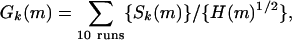where {} means evaluated for a single run. A grandmother cell to recognize the locations similar to m should therefore receive excitatory synapses of equal strength from the subset of layer II neurons that are reliable responders in time bin m. The cell should have a time constant equal to the time bin size. The cell should have shunting inhibition (dividing inhibition) from a global inhibitory signal involving all of the neurons, and that inhibition should be shaped so as to approximate the square root of the total activity of the layer II cells. The input to the grandmother neuron as a function of time will then be a single-run term in the sum (1). Given an appropriate threshold, the only significant difference between using the spikes generated by the grandmother cell and or thresholding Sim_k(m) to find locations m similar to k is that the grandmother cell makes a threshold decision on a trial-by-trial basis, whereas Sim_k(m) thresholds a 10-trial average. Graded excitatory synapse strengths are not needed. The form of the global inhibition is not critical; 1/H(m)^1/2 can be replaced by the more realistic form 1/(1 + B H(m)) or by an additive inhibitory current.

References

- 1.Hopfield, J. J. (1995) Nature 376, 33-36. [DOI] [PubMed] [Google Scholar]
- 2.Brody, C. D. & Hopfield, J. J. (2003) Neuron 37, 843-852. [DOI] [PubMed] [Google Scholar]
- 3.Hopfield, J. J. & Brody, C. D. (2004) Proc. Natl. Acad. Sci. USA 101, 337-342. [DOI] [PMC free article] [PubMed] [Google Scholar]
- 4.Strogatz, S. H. (1994) Non-linear Dynamics and Chaos (Addison Wesley, Reading, MA) 366-368.
- 5.Hopfield, J. J. and Brody, C. D. (2001) Proc. Natl. Acad. Sci. USA 98, 1282-1287. [DOI] [PMC free article] [PubMed] [Google Scholar]
- 6.Junqua, J.-C. & Haton, J.-P. (1996) Robustness in Automatic Speech Recognition (Kluwer Academic, Boston) 28, 235-236. [Google Scholar]
- 7.Shannon, R. V., Zeng, F-G., Kamath, V., Wygonski, J., and Mekelid, M. (1997) Science 270, 303-304. [DOI] [PubMed] [Google Scholar]
- 8.Ehret, G. (1997) J. Comp. Physiol. A 181, 547-557. [DOI] [PubMed] [Google Scholar]
- 9.Fantev, V., Hoke, M., Lehnertz, K. & Lutkenhoner, B. (1989) Electroenecphalogr. Clin. Neurophysiol. 72, 225-231. [DOI] [PubMed] [Google Scholar]
- 10.Hopfield, J. J. and Brody, C. D. (2000) Proc. Natl. Acad. Sci. USA 97, 13919-13924. [DOI] [PMC free article] [PubMed] [Google Scholar]
- 11.Brett, B. & Barth, D. S. (1997) J. Neurophysiol. 78, 573-581. [DOI] [PubMed] [Google Scholar]
- 12.De Weese, M. R., Wehr, M. & Zador, A. M. (2003) J. Neurosci. 23, 7940-7949. [DOI] [PMC free article] [PubMed] [Google Scholar]
- 13.Ohala, J. J. (1985) in Linguistics and Automatic Processing of Speech, NATO Advanced Study Institute series F, eds. De Mori, R. & Suen, C. Y (Springer, Berlin), Vol 16, p. 461. [Google Scholar]
- 14.Rabiner, L. R. & Juang, B.-H. (1993) Fundamentals of Speech Recognition (Prentice Hall, Englewood, NJ) 115-117,163-171.
- 15.Milne, A. A. (1926), Winnie-the-Pooh (Dutton, New York) 1988 Ed., pp. 24-25.