

Abstract
The aim of the study was to establish a parametric transfer function to describe the relationship between ocular perfusion pressure (OPP) and blood flow (BF) in the optic nerve head (ONH). A third-order parametric theoretical model was proposed to describe the ONH OPP-BF relationship within the lower OPP range of the autoregulation curve (< 80 mmHg) based on experimentally induced BF response to a rapid intraocular pressure (IOP) increase in 6 rhesus monkeys. The theoretical and actual data fitted well and suggest that this parametric third-order transfer function can effectively describe both the linear and nonlinear feature in dynamic and static autoregulation in the ONH within the OPP range studied. It shows that the BF autoregulation fully functions when the OPP was > 40 mmHg and becomes incomplete when the OPP was < 40 mmHg. This model may be used to help investigating the features of autoregulation in the ONH under different experimental conditions.
Keywords: Optic nerve head, autoregulation, intraocular pressure, transfer function
Introduction
Blood flow (BF) autoregulation (AR) is an intrinsic ability of the retina and optic nerve head (ONH), among many other bodily tissues, to maintain a relatively constant level of blood in response to variations in perfusion pressure and metabolic demand [1-3]. This process involves multiple mechanisms that may fail as a part of pathogenic processes e.g. glaucoma [2,4-7]. Thus, assessment of autoregulation capacity in ocular tissues is important to understand the mechanisms of the disease and to establish potential therapeutic targets.
The classic method to assess autoregulation capacity within ocular tissue is to compare BF changes before and after ocular perfusion pressure (OPP) is altered, by manipulation of either arterial blood pressure (BP) or intraocular pressure (IOP) [6,8-11]. After this induced OPP change, autoregulation proceeds chronologically in two phases: dynamic (dAR) and static (sAR). During the dAR phase, the pressure change evokes a rapid BF response (increase or decrease), which lasts on average 10-20 sec. When the vascular resistance and BF stabilizes to either its original or a new level, the sAR phase is then reached [12]. A series of BF changes measured during the sAR phase in response to varying levels of perfusion pressure constitute a classic AR curve, or P-F relationship [1] as demonstrated in Figure 1.
Figure 1.

A schematic view of the relationship between OPP and BF. The middle segment of the curve represents the autoregulation range, within which the autoregulation remains effective. When OPP fluctuations exceed this range, i.e. higher than the upper or lower than the lower limit, BF will passively increase or decrease.
Whilst sAR analysis utilizes the BF change in amplitude before and after the OPP change, analysis of the dAR phase includes both amplitude and time latencies [13]. Thus, dAR analysis has been considered as a more effective clinical method at revealing potential autoregulation dysfunction, as demonstrated in ischemic and traumatic brain injuries [14-18]. Yet, previous studies relating to ocular autoregulation have focused on sAR, and overlooked the dAR component.
The inherent complexities of BF AR encourage the use of mathematical modeling. Utilizing the mechanistic features of autoregulation, discrepancies between theoretical systems behaviors and actual behaviors measured in vivo can point to hitherto unknown components that are missing, thereby assisting in developing a more comprehensive picture of this biological process. However, there are limited BF AR mathematical models [19,20] and few studies specifically focusing on the eye [3,21]. One of the difficulties applying a mathematic model to describe autoregulation capacity is the nonlinearity of the relationship between BF response and OPP [22].
Previously, first-order linear time-invariant transfer functions have been used for analysis of dAR. However, most of these first-order linear models are focused specifically upon the plateau region of the autoregulation curve [22,23]. Consequently, grading the autoregulatory response is limited to either, the lower or upper critical points of the autoregulation curve or the shifts of the curve by altering the physiological parameters.
Second-order transfer functions, designed within the scenario of spontaneous BP fluctuations have been used to represent the properties of BF autoregulation in which the perfusion pressure changes do not extend to the nonlinear range of the autoregulation curve, though it is adequate to describe the descending phase and the steady state of the BF response, the model is too rigid to depict the gradually ascending property during recovery so that it describes only the linear property of autoregulation but not the full course of autoregulation from dAR phase to sAR.
As such, a higher order of differential model may be more appropriate to represent the autoregulation pattern since it is capable of providing more flexibility to describe both the linear and nonlinear features of autoregulation during the BF response. In our previous study [24], it has shown that the magnitude of both maximal dAR change and the steady state BF are closely related to the IOP and BP and for both dAR and sAR, the OPP is a determining factor to mediate the interaction between sAR and dAR. To incorporate sAR and dAR into a single model, BF response to variations of different OPP need to be assessed.
To accomplish the previously stated goals a theoretical third-order parametric model was established to describe the OPP-BF relationship incorporating both dAR and sAR. This model was then validated utilizing in vivo data, where the ONH dAR and sAR responses were induced by rapidly increasing the IOP. The resultant parametric transfer function may serve as a tool to predict and gauge the impairment of autoregulation in disease conditions and may have a potential application to assess the autoregulation capacity in humans.
Materials and methods
Quantification of rapid IOP increase induced BF autoregulation in ONH
Six male rhesus (Macaca mulatta) monkeys without observable eye diseases, ranging from 9 to 12 (10.7 ± 1.4, mean ± SD) years old and weighing 5.6 to 13 kg (10.1 ± 3.4 kg), were used. All experimental protocols and animal care procedures adhered to the ARVO Statement for the Use of Animals in Ophthalmic and Vision Research and were approved by the Legacy Research Institutional Animal Care and Use Committee.
The animal was sedated initially by an intramuscular injection of ketamine/xylazine (15 mg.kg-1 and 0.8 mg.kg-1); anesthesia was maintained thereafter by continuous administration of pentobarbital (6-9 mg.kg-1.hour-1, IV) using an infusion pump (Aladdin, World Science Instruments Inc., Sarasota, FL). Pentobarbital was selected because this anesthetic, unlike the volatile gas anesthetics [18,25], has minimal impact on autoregulation capacity [26-28]. Animals were intubated and breathed with room air.
The animal was placed on a table in prone position. Body temperature was maintained with a 37°C circulating warm-water heating pad. Pulse rate and oxygen saturation were monitored continuously (Propaq Encore model 206EL; Protocol Systems, Inc., Beaverton, OR) and maintained between 85-125 per minute and O2 above 95%, respectively. One of the superficial arteries in a leg was cannulated with a 27G needle, which was connected to a pressure transducer (BLPR2, WPI, NH) and a four-channel amplifier system (Lab-Trax-4/24T, WPI, NH). BP in the artery was recorded continuously and stored into a computer.
A laser speckle flowgraphy (LSFG. Softcare, Japan) device was used to estimate the BF in the ONH. In brief, a fundus camera equipped within the LSFG device was focused on an area centered on the ONH. The area is approximately 3.8 mm x 3 mm (Width x Height). After the laser is switched on (λ = 830 nm, maximum output power, 1.2 mW), a speckle pattern is generated due to random interference of the scattered light from the illuminated tissue area. The speckle pattern is continuously imaged by a charge coupled device (700 x 480 pixels) at a frequency of 30 frames per second for 4 seconds at a time. Offline analysis software (LSFG Analysis, Softcare, Iizuka, Japan) computed a mean blur rate (MBR) of the speckle images. MBR is a squared ratio of mean intensity to the standard deviation of light intensity of the image, which varies temporally and spatially according to the velocity of blood cells movement and correlates well with capillary BF within the ONH validated by the microsphere [29] and the hydrogen clearance methods [30]. Thus, the MBR has been used as a BF index. A composite MBR map representing BF distribution within the ONH disc was generated from the images of each 4-second series. After eliminating the area corresponding to large blood vessels within the images, capillary BF within the remaining ONH disc area was averaged and reported in arbitrary units (A.U.) of MBR.
Manometrical IOP control and recording
Two 27G needles were inserted into the anterior chamber of the eye via the temporal corneoscleral limbus. One of the two needles was connected to a pressure transducer to register the IOP; the other needle was connected to either one of two sterile saline reservoirs, each set at a different height. The connection of the reservoirs to the anterior chamber was controlled by a solenoid valve (Valcor Engineering, Springfield, NJ), which allows one of the reservoirs to be opened and the other closed so that the IOP can be changed from one level to the other nearly instantaneously. A computer mouse synchronized the valve control with the BF measurement program. The OPP was computed using the equation OPP = BP – IOP – 5 (mmHg), where 5 mmHg is the height difference from eye to heart when the animal was in a prone position.
IOP step increase induced sAR and dAR responses
Under a range of BP between 80 and 95 mmHg and IOP set manometrically at 10 mmHg, baseline ONH BF images was acquired by the LSFG. Ten seconds after the completion of baseline imaging, the electronic valve connected to a saline reservoir at a height equivalent to either 30 or 40 or 50 mmHg (IOP1030; IOP1040; IOP1050 respectively) was switched open by the synchronized computer mouse to induce a rapid IOP change. The BF recording continued for 60 seconds and, thereafter, for 10 seconds every minute for a total of 5 minutes. The above tests were repeated three times in both eyes of the 6 animals (12 eyes) to obtain the empirical BF response at varied OPPs. The percentage difference of BF between the baseline value and that at the end of 5 min of IOP increase was calculated as sAR. All the sAR measured over different OPPs was used for the construction of the autoregulation curve and the subsequent mathematic modeling.
Mathematical modeling of autoregulation system
As the schematically illustrated OPP-BF relationship, or sAR autoregulation curve shown in Figure 1, a plateau covers a range of OPP where the autoregulation remains effective. When the OPP exceeds the critical range defined by this plateau, i.e. beyond the upper and below lower limits of the AR range, BF will passively become either greater or lower following the OPP changes.
Because BF autoregulation is not a simple response to a mechanical stimulus, but also to different chemical and biological stimuli through a variety of scales and pathways, thus complicates efforts to represent it. In order to simplify the mathematical analysis of the system, all procedures could be described as an input-output model (black-box) between OPP and BF (Figure 2). Subsequently, a linear or nonlinear transfer function, in terms of spatial or temporal frequency, can be derived to depict the relationship between OPP and BF. The transfer function then can be estimated using a system identification method or curve fitting from a series of experimental measurements.
Figure 2.
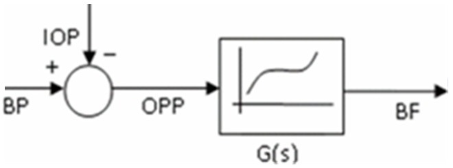
Simplified transfer function representation of the relationship between BF and OPP. Where the OPP is considered as an input, determined by both BP and IOP, and utilizing the black box system, the BF or the output is processed and exported.
The transfer function in Figure 2 can be expressed as a quotient of polynomials
G(s) = p(s)/q(s) = (bmsm+…+b 1 s+b 0)/(ansn+…+a 1 s+a 0), n ≥ m (1)
where s is the Laplace operator; n ≥ m according to the initial value theorem and final value theorem [31].
Considering the model is an approximation of a physiology procedure, the degree of activation of the vascular smooth muscle arising through the myogenic mechanism is given by a first order transfer function [32,33]:
G 1 (s) = k 1/(Tps+1) (2)
where k 1 is the regulation gain and Tp the time constant.
Based on published models on transfer function analysis, the degree of activation arising through the metabolic and other mechanisms was hypothesized to fit by a second order transfer function of the form [34,35].
G 2 (s) = k 2/(1+2ζTws+Tw 2 s 2) (3)
where k 2 is regulation gain, Tw is a time constant, and ζ is the damping ratio.
Combining the two procedures, the autoregulation procedure of BF could be expressed by a third-order transfer function of the form:
BF/OPP = G(s) = KP/(1+2ζTws+Tw 2 s 2)(1+Tps) (4)
where Kp = k 1 k 2.
To verify the validity of the third order model, we analyzed the experimental data from six monkeys. This third order system conformed to the model prepared from in vivo measurements as shown in Figure 3. When applying the same input to the theoretical model with parameters Kp = 0.03, Tp = 14.46, Tw = 2.54, ζ = 1.20 in Equation 4, the output of the transfer function model (simulated BF) correlates with the in vivo experimental output (measured BF) as illustrated in Figure 4.
Figure 3.

A typical recording of OPP (calculated based on the BP and IOP) and BF response. A: IOP was acutely increased from 10 mmHg to 40 mmHg, starting at the 10th second and induced an OPP decrease from 76 to 46 mmHg; B: BF decreases correspondingly during the initial OPP decrease for approximately 10-15 seconds (dAR phase) and then gradually returns towards a stabilized level (sAR).
Figure 4.

The simulated BF response (red dotted) fits with the in vivo BF response (solid black). In this typical example, the IOP was increased from 10 mmHg to 40 mmHg. As shown in the 60 seconds recording (solid black curve), BF response induced by this IOP increase underwent dAR and sAR phases. The simulated BF response by the parametric transfer function was fitted well with the experimental derived BF response.
BF autoregulation is clearly a nonlinear phenomenon, thus, a linear approximation of a nonlinear model can be justified in a small range of OPP around a point of equilibrium by utilizing the segmental linear property of the autoregulation curve without altering the features of the curve. Therefore, a piecewise linear transfer function, i.e., a parametric transfer function, was used to describe the static and dynamic properties of autoregulation under different OPP. Since BF is a nonlinear function of OPP, the OPP level can be used as a parametric input of the piecewise transfer function, that is, each parameter in Equation 4 could be described as a function of the OPP level. Defining x as an independent variable representing the OPP level, it is possible to find the functions Kp = f 1 (x), Tp = f 2 (x), Tw = f 3 (x), and ζ = f 4 (x), from experimental data to complete the parametric transfer function over the full range of OPP. All values of Kp at a full range of OPP, is composed of the static autoregulation curve from the final value theory of linear system step response. In the scenario of this study, the OPP was limited to the lower half of the autoregulation curve (OPP < 80 mmHg) since BP was from 80 mmHg to 100 mmHg in all experiments.
Results
Quantification of rapid IOP increase induced BF autoregulation in ONH
Static BF autoregulation curve of ONH
Due to varied BP in animals during each test, the IOP increase from 10 mmHg to either 30, 40 or 50 mmHg resulted in a range of OPP decrease between 15 and 67 mmHg. The percentage BF change after IOP elevation normalized to their baseline values are plotted against each corresponding OPP to construct portion of a complete autoregulation curve as shown in Figure 5.
Figure 5.

The sAR measured at a range of OPP. Each data point (averaged from three repeated measures) represents the sAR at a given level of OPP. The data is best fit with a polynomial function. Since the highest OPP in these anesthetized animals can only be reached to a certain level below 70 mmHg, the curve represents only a portion of the autoregulation curve within the lower OPP range.
The BF and OPP were fitted to a polynomial function to describe the static relationship between OPP (x) and BF (yBF) at the lower half (OPP < 70 mmHg) of the static autoregulation curve:
yBF = 7.6 × 10-6 x 3 – 1.1 × 10-3 x 2 + 5.6 × 10⁻² x (P<0.0001, r=0.8) (5)
The shape of the fitted curve resembles the theoretical autoregulation curve in the lower half of OPP shown in Figure 1. In the curve, BF maintained at a constant level when the OPP was higher than 40 mmHg, reflecting BF recovering to baseline completely and a fully functional autoregulation. When the OPP was below 40 mmHg, BF decreased with the decrease of OPP, indicating an incomplete recovery.
Parameters of transfer function
Figure 6 shows the four parameters (Kp, Tp, Tw and ζ) in Equation 4 estimated from the experiments measured at different OPP levels. The data points of each parameter in Figure 6 were derived from the measured BF curves at a different range of OPP (see Figure 4). Each parameter was fitted to a polynomial function of the OPP (x) at steady state:
Figure 6.

Estimations of Kp, Tp, Tw and ζ from experimental data. Each parameter is a nonlinear function of OPP to gain (A), the time constants Tp (B) and Tw (C), and a damping ratio ζ (D).
Kp = 1.31 × 10-5 x 2 – 1.5 × 10⁻³ x + 6.15 × 10⁻² (P<0.0001, r=0.94) (6)
Tp = 9.9 × 10-3 x 2 – 0.347x + 12.50 (P<0.0001, r=0.85) (7)
Tw = 6.9 × 10-4 x 2 – 0.0852x + 4.84 (P<0.0001, r=0.69) (8)
ζ = 2.41 × 10-4 x 2 – 0.047x + 2.69 (P<0.0001, r=0.92) (9)
In Figure 6A, the gain of the transfer function (Kp) has a nonlinear relationship with OPP, which decreases when OPP increases and reaches a constant when OPP is above a certain value. Panel B and Panel C illustrate the relationship of the two time constants (Tp and Tw) with the OPP. Tp increases monotonically with OPP and approaches to a constant of 10 sec when OPP becomes lower than 25 mmHg. Tw is a monotonically descendant function of OPP and converges to a value of 2.5 seconds when OPP is above 50 mmHg. Tw is relative stable and varies in a range of 1.7-3.8 seconds. The damping ratio ζ is a quasi-linear function of OPP and monotonically decreasing with OPP; the lower the OPP, the lower the damping ratio.
Dynamic autoregulation time duration
In order to find out the dynamic duration of the BF autoregulation, BF measured at 45 seconds and 55 seconds were compared with averaged BF measured from 4-5 minutes, as shown in Table 1. Since BF stabilizes at approximately a constant after 5 minutes, averaged BF measured from 4-5 minute can be readily assumed as final value. At 45 seconds, the BF reached a state which was less than 5% variation from the steady state (2 ± 3% and 4 ± 1% for IOP1030 and IOP1040, respectively). If a percentage variation of ± 5% from the final value was considered a new steady state, it is reasonable to conclude that the dynamic autoregulation happened in duration of about 1 min; thus, a continuous time course measurement of BF of 1 min provides enough spatial resolution for dynamic analysis.
Table 1.
Percentage change of BF at 45 sec and 55 sec compared to 5 min under IOP1030 and IOP1040
| IOP | BF deviation at 45 sec | BF deviation at 55 sec |
|---|---|---|
| 10-30 mmHg | 2 ± 3% | 2 ± 3% |
| 10-40 mmHg | 3 ± 1% | 4 ± 1% |
IOP: intraocular pressure; BF: blood flow.
The transient changes of OPP induced by different IOP elevations, the experimentally and predicted BF changes are presented in Figure 7. The OPP was considered as the input of transfer function and the parameters of the transfer functions were calculated from Equations 6 to 9 using the steady state OPP of each mean. The simulated BF followed the mean in vivo BF, suggesting that the transient BF change under different OPPs can be modeled by a parametric transfer function even though autoregulation is nonlinear to OPP.
Figure 7.

Comparison of predicted transient BF responses with the measured BF responses during OPP lowing. The OPP was reduced manometrically by IOP1030 (A), IOP1040 (B) and IOP1050 (C), respectively (top panels). The BF responses at each corresponding OPP decrease are shown in bottom panels. The broken red lines are the BF responses simulated by the parametric transfer function. The solid blue lines are mean BF responses obtained experimentally from the 6 animals (solid lines = mean, dotted lines = SD).
Discussion
In this study, a mathematical model was developed that utilized a parametric transfer function to analyze the relationship between BF and OPP following acute IOP elevations. This transfer function consists of 4 parameters: gain Kp, time constant Tp, time constant Tw and a damping ratio, ζ. The real parts of all poles of the denominator within Equation 4 are negative, which requires that ζ > 0. This criterion is satisfied as long as OPP < 80 mmHg, as shown in Figure 6D.
The gain Kp is a monotonically decreasing function of the OPP and is directly related to the recovery rate of the BF in the steady state. After the transient phase of the BF response following IOP elevation, Kp is the only functional parameter in this model; and it resembles the capability of static autoregulation. The higher the value of Kp, the less the BF recovers to the baseline.
The first-order model represents the response time of the vascular muscle after acute OPP drop [33,36]. Tp is the only parameter in this equation monotonically increasing function of OPP. From system simulation, it is found that a smaller Tp reproduces a bigger change of BF and strongly regulated the BF back to the baseline. This complies with the phenomenon that a larger drop of OPP resulting in larger BF decrease and consequently stronger recovery. Therefore, the parameter Tp likely represents the strength of the vascular muscle and depicts the myogenic process of the BF response following IOP elevation.
Two parameters, Tw and ζ, are involved in the second-order model. Tw was a monotonically decreasing function of OPP and varied in a range of 2-4 sec. Compared with the wide range variation of Tp, it may be applicable to limit Tw as a constant of 3 second and thus to assume the second-order model is more related to the metabolic process. ζ is an unvarying decreasing function of OPP and was a damping ratio of second-order equation from simulation. However, from the facts of dynamic response of BF, ζ means more than a damping ratio since it also reflects the regulation strength in the second-order model. In system simulation it is well known that higher ζ indicates higher damping thus less overshoot. In a scenario where bigger drop of OPP results in bigger BF decrease; considering only the activities of the vascular muscle in the recovery period, the BF will recover quicker with the consequence of higher overshoot. However, in all experiments no such overshoot was observed; this leads to the assumption that a high value of ζ exerted to yield the overshoot of the BF. The assumption is consistent to the estimation results that OPP drop is proportional to value of ζ. Since ζ functions dominantly in the recovery period, it might be very informative when exploring the autoregulation in pathological condition.
Our previous study introduced factors affecting the normal pattern of dAR and sAR including the magnitude of the stimuli (IOP), the response time, the magnitude of BF response and the recovery rate [24]. These multiple factors interact with each other and obscure the interpretation of whether an autoregulation response is normal. The transfer function provided a method to detect the early or moderate change of dynamic response of certain pathologies by comparing the parameters of transfer function estimated from pathological condition and control condition.
The challenge of modeling a physiological system mathematically is to balance its predictive capability and its simplicity to enable interpretation of the physiology dynamics. There must also be a balance between the scope of questions posed and comprehensiveness of the model. The first limitation of the model is that the parameters of this model were limited to an OPP less than 80 mmHg since the regression of all curves were performed under OPP 80 mmHg. Clearly, the model applies to dynamic autoregulation caused by an acute IOP elevation or an acute BP decrease, but is not applicable to a spontaneous fluctuation of OPP. The second limitation is that this model does not specify each parameter with the underlying physiological processes. The first-order differential equation likely represents the action of vascular smooth muscle [33], but the second-order differential equation may better correspond with the processes [34,37]; more than metabolic mechanism, which remains to be determined in future work. The other limitation is the use of multiple parameters) to simulate spatially distributed hemodynamics, i.e., the parametric linear approximation of the autoregulation curve. Clearly the predicted BF autoregulation is just an approximation around small equilibrium points, but it enables valuable data to be extrapolated from the experimental data.
As has been noted above, the ocular BF autoregulation system is more complex than the parametric transfer function presented in this study. However, one of the advantages of the parametric transfer function is that it describes the relationship between OPP and BF not only within the linear range but also in the nonlinear range of autoregulation. In addition, it predicts the quantitative BF change over a range of OPP that represents the systematic property of BF autoregulation. Though this estimated parametric transfer function cannot to be phrased as a theorem, the model gives reasonable behavior despite many uncertainty and inaccuracies in parameter estimation. Presumably it reflects the fact that the biological system have evolved to be robust.
Conclusions
The simulated BF response within the transfer function model corroborated the in vivo measured BF response in not only static autoregulation but also within the dynamic autoregulation. Thus, a parametric third-order transfer function can effectively describe the ONH BF autoregulation following IOP elevation, because it illustrates the linear and nonlinear features of autoregulation and predicts quantitative BF change over a wide range of OPPs. Future studies may extend the application of the model to investigate the effect of physiological variation such as aging effects and blood pressure induced OPP changes in BF autoregulation.
Acknowledgements
The study was supported by NIH EY019939 (LW); non restriction fund from Translational Medicine, Pfizer Inc. (LW); Good Samaritan Foundation (LW); Reserve Talents of Universities Overseas Research Program of Heilongjiang by Heilongjiang Education Department, P R China (JY).
Disclosure of conflict of interest
None.
References
- 1.Bill A, Sperber GO. Aspects of oxygen and glucose consumption in the retina: effects of high intraocular pressure and light. Graefes Arch Clin Exp Ophthalmol. 1990;228:124–127. doi: 10.1007/BF00935720. [DOI] [PubMed] [Google Scholar]
- 2.Anderson DR. Introductory comments on blood flow autoregulation in the optic nerve head and vascular risk factors in glaucoma. Surv Ophthalmol. 1999;43(Suppl 1):S5–9. doi: 10.1016/s0039-6257(99)00046-6. [DOI] [PubMed] [Google Scholar]
- 3.Arciero J, Harris A, Siesky B, Amireskandari A, Gershuny V, Pickrell A, Guiodoboni G. Theoretical analysis of vascular regulatory mechanisms contributing to retinal blood flow autoregulation. Invest Ophthalmol Vis Sci. 2013;54:5584–5593. doi: 10.1167/iovs.12-11543. [DOI] [PMC free article] [PubMed] [Google Scholar]
- 4.Spaeth GL. Fluorescein angiography: its contributions towards understanding the mechanisms of visual loss in glaucoma. Trans Am Ophthalmol Soc. 1975;73:491–553. [PMC free article] [PubMed] [Google Scholar]
- 5.Harris A, Kagemann L, Cioffi GA. Assessment of human ocular hemodynamics. Surv Ophthalmol. 1998;42:509–533. doi: 10.1016/s0039-6257(98)00011-3. [DOI] [PubMed] [Google Scholar]
- 6.Li G, Shih YY, Kiel JW, De La Garza BH, Du F, Duong TQ. MRI study of cerebral, retinal and choroidal blood flow responses to acute hypertension. Exp Eye Res. 2013;112:118–124. doi: 10.1016/j.exer.2013.04.003. [DOI] [PMC free article] [PubMed] [Google Scholar]
- 7.Cherecheanu AP, Garhofer G, Schmidl D, Werkmeister R, Schmetterer L. Ocular perfusion pressure and ocular blood flow in glaucoma. Curr Opin Pharmacol. 2013;13:36–42. doi: 10.1016/j.coph.2012.09.003. [DOI] [PMC free article] [PubMed] [Google Scholar]
- 8.Bill A. Blood circulation and fluid dynamics in the eye. Physiol Rev. 1975;55:383–417. doi: 10.1152/physrev.1975.55.3.383. [DOI] [PubMed] [Google Scholar]
- 9.Pournaras CJ. Autoregulation of ocular blood flow. In: Kaiser HJ, Flammer J, Hendrickson P, editors. Ocular Blood Flow. Basel: Karger; 1995. pp. 40–50. [Google Scholar]
- 10.Michelson G, Groh MJ, Langhans M. Perfusion of the juxtapapillary retina and optic nerve head in acute ocular hypertension. Ger J Ophthalmol. 1996;5:315–321. [PubMed] [Google Scholar]
- 11.Weigert G, Findl O, Luksch A, Rainer G, Kiss B, Vass C, Schmetterer L. Effects of moderate changes in intraocular pressure on ocular hemodynamics in patients with primary open-angle glaucoma and healthy controls. Ophthalmology. 2005;112:1337–1342. doi: 10.1016/j.ophtha.2005.03.016. [DOI] [PubMed] [Google Scholar]
- 12.Quaranta L, Manni G, Donato F, Bucci MG. The effect of increased intraocular pressure on pulsatile ocular blood flow in low tension glaucoma. Surv Ophthalmol. 1994;38(Suppl):S177–181. doi: 10.1016/0039-6257(94)90064-7. discussion S182. [DOI] [PubMed] [Google Scholar]
- 13.Panerai RB. Transcranial Doppler for evaluation of cerebral autoregulation. Clin Auton Res. 2009;19:197–211. doi: 10.1007/s10286-009-0011-8. [DOI] [PubMed] [Google Scholar]
- 14.Dineen NE, Brodie FG, Robinson TG, Panerai RB. Continuous estimates of dynamic cerebral autoregulation during transient hypocapnia and hypercapnia. J Appl Physiol. 2010;108:604–613. doi: 10.1152/japplphysiol.01157.2009. [DOI] [PMC free article] [PubMed] [Google Scholar]
- 15.Panerai RB. Cerebral autoregulation: from models to clinical applications. Cardiovasc Eng. 2008;8:42–59. doi: 10.1007/s10558-007-9044-6. [DOI] [PubMed] [Google Scholar]
- 16.Panerai RB, Chacon M, Pereira R, Evans DH. Neural network modelling of dynamic cerebral autoregulation: assessment and comparison with established methods. Med Eng Phys. 2004;26:43–52. doi: 10.1016/j.medengphy.2003.08.001. [DOI] [PubMed] [Google Scholar]
- 17.Panerai RB, Kelsall AW, Rennie JM, Evans DH. Analysis of cerebral blood flow autoregulation in neonates. IEEE Trans Biomed Eng. 1996;43:779–788. doi: 10.1109/10.508541. [DOI] [PubMed] [Google Scholar]
- 18.Tiecks FP, Lam AM, Aaslid R, Newell DW. Comparison of static and dynamic cerebral autoregulation measurements. Stroke. 1995;26:1014–1019. doi: 10.1161/01.str.26.6.1014. [DOI] [PubMed] [Google Scholar]
- 19.Sgouralis I, Layton AT. Autoregulation and conduction of vasomotor responses in a mathematical model of the rat afferent arteriole. American journal of physiology. Renal physiology. 2012;303:F229–239. doi: 10.1152/ajprenal.00589.2011. [DOI] [PMC free article] [PubMed] [Google Scholar]
- 20.Niijima T, Aso Y, Akaza H, Fujita K, Fuse H, Hosaka M, Isurugi K, Kamidono S, Katayama T, Kawabe K, et al. [Clinical phase I and phase II study on a sustained release formulation of leuprorelin acetate (TAP-144-SR), an LH-RH agonist, in patients with prostatic carcinoma. Collaborative++ Studies on Prostatic Carcinoma by the Study Group for TAP-144-SR] . Hinyokika Kiyo. 1990;36:1343–1360. [PubMed] [Google Scholar]
- 21.Harris A, Guidoboni G, Arciero JC, Amireskandari A, Tobe LA, Siesky BA. Ocular hemodynamics and glaucoma: the role of mathematical modeling. Eur J Ophthalmol. 2013;23:139–46. doi: 10.5301/ejo.5000255. [DOI] [PMC free article] [PubMed] [Google Scholar]
- 22.Giller CA, Mueller M. Linearity and non-linearity in cerebral hemodynamics. Med Eng Phys. 2003;25:633–646. doi: 10.1016/s1350-4533(03)00028-6. [DOI] [PubMed] [Google Scholar]
- 23.Zhang R, Zuckerman JH, Giller CA, Levine BD. Transfer function analysis of dynamic cerebral autoregulation in humans. Am J Physiol. 1998;274:H233–241. doi: 10.1152/ajpheart.1998.274.1.h233. [DOI] [PubMed] [Google Scholar]
- 24.Liang Y, Downs JC, Fortune B, Cull GA, Cioffi GA, Wang L. Impact of Systemic Blood Pressure on the Relationship between Intraocular Pressure and Blood Flow in the Optic Nerve Head of Non-Human Primates. Invest Ophthalmol Vis Sci. 2009;50:2154–2160. doi: 10.1167/iovs.08-2882. [DOI] [PubMed] [Google Scholar]
- 25.Werner C, Lu H, Engelhard K, Unbehaun N, Kochs E. Sevoflurane impairs cerebral blood flow autoregulation in rats: reversal by nonselective nitric oxide synthase inhibition. Anesth Analg. 2005;101:509–516. doi: 10.1213/01.ANE.0000160586.71403.A4. [DOI] [PubMed] [Google Scholar]
- 26.Kremser PC, Gewertz BL. Effect of pentobarbital and hemorrhage on renal autoregulation. Am J Physiol. 1985;249:F356–360. doi: 10.1152/ajprenal.1985.249.3.F356. [DOI] [PubMed] [Google Scholar]
- 27.Preckel MP, Leftheriotis G, Ferber C, Degoute CS, Banssillon V, Saumet JL. Effect of nitric oxide blockade on the lower limit of the cortical cerebral autoregulation in pentobarbital-anaesthetized rats. Int J Microcirc Clin Exp. 1996;16:277–283. doi: 10.1159/000179186. [DOI] [PubMed] [Google Scholar]
- 28.Paterno R, Heistad DD, Faraci FM. Potassium channels modulate cerebral autoregulation during acute hypertension. Am J Physiol Heart Circ Physiol. 2000;278:H2003–2007. doi: 10.1152/ajpheart.2000.278.6.H2003. [DOI] [PubMed] [Google Scholar]
- 29.Wang L, Cull GA, Piper C, Burgoyne CF, Fortune B. Anterior and posterior optic nerve head blood flow in nonhuman primate experimental glaucoma model measured by laser speckle imaging technique and microsphere method. Invest Ophthalmol Vis Sci. 2012;53:8303–8309. doi: 10.1167/iovs.12-10911. [DOI] [PMC free article] [PubMed] [Google Scholar]
- 30.Takahashi H, Sugiyama T, Tokushige H, Maeno T, Nakazawa T, Ikeda T, Araie M. Comparison of CCD-equipped laser speckle flowgraphy with hydrogen gas clearance method in the measurement of optic nerve head microcirculation in rabbits. Exp Eye Res. 2013;108:10–15. doi: 10.1016/j.exer.2012.12.003. [DOI] [PubMed] [Google Scholar]
- 31.Fox JG, Anderson LC, Loew FM, Quimby FW. Laboratory Animal Medicine. San Diego: Academic Press; 2002. [Google Scholar]
- 32.Banaji M, Tachtsidis I, Delpy D, Baigent S. A physiological model of cerebral blood flow control. Math Biosci. 2005;194:125–173. doi: 10.1016/j.mbs.2004.10.005. [DOI] [PubMed] [Google Scholar]
- 33.Holstein-Rathlou NH, Marsh DJ. A dynamic model of renal blood flow autoregulation. Bull Math Biol. 1994;56:411–429. doi: 10.1007/BF02460465. [DOI] [PubMed] [Google Scholar]
- 34.Diamond SG, Perdue KL, Boas DA. A cerebrovascular response model for functional neuroimaging including dynamic cerebral autoregulation. Math Biosci. 2009;220:102–117. doi: 10.1016/j.mbs.2009.05.002. [DOI] [PMC free article] [PubMed] [Google Scholar]
- 35.Payne SJ, Tarassenko L. Combined transfer function analysis and modelling of cerebral autoregulation. Ann Biomed Eng. 2006;34:847–858. doi: 10.1007/s10439-006-9114-8. [DOI] [PubMed] [Google Scholar]
- 36.Kleinstreuer N, David T, Plank MJ, Endre Z. Dynamic myogenic autoregulation in the rat kidney: a whole-organ model. Am J Physiol Renal Physiol. 2008;294:F1453–F1464. doi: 10.1152/ajprenal.00426.2007. [DOI] [PubMed] [Google Scholar]
- 37.Rieger JW, Gegenfurtner KR, Schalk F, Koechy N, Heinze HJ, Grueschow M. BOLD responses in human V1 to local structure in natural scenes: Implications for theories of visual coding. J Vis. 2013;13:19. doi: 10.1167/13.2.19. [DOI] [PubMed] [Google Scholar]