

Abstract
Fluorescence tomography (FT) is a promising molecular imaging technique that can spatially resolve both fluorophore concentration and lifetime parameters. However, recovered fluorophore parameters highly depend on the size and depth of the object due to the ill-posedness of the FT inverse problem. Structural a priori information from another high spatial resolution imaging modality has been demonstrated to significantly improve FT reconstruction accuracy. In this study, we have constructed a combined magnetic resonance imaging (MRI) and FT system for small animal imaging. A photo-multiplier tube (PMT) is used as the detector to acquire frequency domain FT measurements. This is the first MR-compatible time-resolved FT system that can reconstruct both fluorescence concentration and lifetime maps simultaneously. The performance of the hybrid system is evaluated with phantom studies. Two different fluorophores, Indocyanine Green (ICG) and 3-3′ Diethylthiatricarbocyanine Iodide (DTTCI), which have similar excitation and emission spectra but different lifetimes, are utilized. The fluorescence concentration and lifetime maps are both reconstructed with and without the structural a priori information obtained from MRI for comparison. We show that the hybrid system can accurately recover both fluorescence intensity and lifetime within 10% error for two 4.2 mm-diameter cylindrical objects embedded in a 38 mm-diameter cylindrical phantom when MRI structural a priori information is utilized.
1. Introduction
Fluorescence tomography (FT) is becoming an important molecular imaging tool to identify biomarker distributions in vivo (Leblond et al. 2010, Ntziachristos 2006, Sevick-Muraca and Rasmussen 2008). It holds promise in many clinical applications such as early disease diagnosis, cancer treatment assessment, and monitoring of cell therapy (Bremer 2008, Bremer et al. 2003, Frangioni 2003, Hoshino et al. 2007). In essence, there are two parameters that can be spatially resolved with this technique, namely the fluorescence concentration and lifetime (Milstein et al. 2003, Nothdurft et al. 2009, Patterson and Pogue 1994). The fluorescence concentration depends on the amount of exogenous fluorescence agent, while the fluorescence lifetime is affected by the local environmental parameters such as the pH value, temperature, and oxygen supply. In recent years, several laboratories have successfully developed fluorescence tomography scanners for small animal imaging, and some have become commercially available (Davis et al. 2008, Kepshire et al. 2009, Koenig et al. 2008, Lin et al. 2010, Nothdurft et al. 2009, Ntziachristos et al. 2003, Tan and Jiang 2008, Venugopal et al. 2010, Zhang et al. 2009). A few FT systems for human breast imaging are also under development (Corlu et al. 2007, Ge et al. 2009, Godavarty et al. 2005a). FT is an imaging modality with high sensitivity but low spatial resolution. The FT inverse problem is severely ill-posed; hence, the recovered fluorophore concentration highly depends on the size and depth of the inclusion (Kepshire et al. 2008, Kepshire et al. 2007, Lin et al. 2010, Lin et al. 2009). In order to improve its accuracy, structural a priori information from another high spatial resolution imaging modality, such as magnetic resonance imaging (MRI) or x-ray computed tomography (XCT), has been utilized to constrain and guide the FT reconstruction (Ale et al. 2010, Davis et al. 2008, Kepshire et al. 2009, Lin et al. 2010).
Based on system design, FT small animal scanners can be categorized into two types: non-contact and contact systems. In general, a charge-coupled device (CCD) is used as the photon detector for the non-contact systems due to the fact that it has the advantage of acquiring a large number of data points at the boundary of the object. Non-contact FT systems have been successfully integrated with XCT systems to achieve more quantitative fluorescence images. In contrast, contact FT systems usually utilize optical fibers to both deliver the excitation light to and collect the emitted light from the boundary of the object. The main advantage of an optical fiber based contact system is its compatibility with an MRI system, since the light detection unit can be placed outside the high magnetic field. There are several advantages of obtaining anatomical a priori information from MRI instead of XCT. Mainly, MRI offers better soft tissue contrast and does not impose ionizing radiation. This is especially important for a small animal imaging system due to the high radiation dose in small animal CT scans.
Up until now, most multi-modality FT systems have only acquired continuous wave measurements, and thus, could measure only the fluorophore concentration. In particular, Davis et al. have implemented an MRI-combined CCD-based continuous-wave (CW) FT system for in vivo small-animal imaging, using spectrograph-coupled CCD detectors (Davis et al. 2008). Significant improvement for the reconstructed fluorophore concentration has been demonstrated using MRI spatial a priori information (Davis et al. 2008). Several combined FT/CT systems have also been developed and the results again showed significant improvement of the FT reconstruction using CT anatomical information. On the other hand, building a time-resolved hybrid system is more challenging due to its complexity. Therefore, even though there have been a few stand alone time-resolved FT systems (Culver et al. 2007, Gao et al. 2010, Godavarty et al. 2005b, Kumar et al. 2008, Milstein et al. 2004, Nothdurft et al. 2009, Soloviev and Arridge 2007), the reconstruction of fluorescence lifetime using anatomical a priori information has not been shown yet. Since both fluorophore concentration and lifetime are essential parameters in FT, the ideal approach is to reconstruct both of them simultaneously. This necessitates time-dependent measurement techniques with MRI compatibility.
Accordingly, we developed a hybrid frequency domain MR-FT system that can acquire FT measurements and MR images simultaneously. The optical interface that is integrated with MR coil provides a perfect co-registration in space and time. Furthermore, successful co-registration of images allows us to utilize MR high resolution anatomical information as priors to guide and constrain the FT reconstruction. The FT system operates in the frequency domain at 100 MHz modulation frequency. A photo-multiplier tube (PMT) is used for optical signal detection. PMTs have very high sensitivity due to their intrinsically high gain. In addition, the fast response time of the PMT make it ideal for time-dependent measurements, which are required to recover the fluorescence lifetime parameter.
The performance of the system was evaluated using phantom studies. We first assessed the linearity of the system response using fluorescence inclusions with various concentrations of fluorophore. Next, size and location dependence of the recovered fluorophore concentration were investigated. For both studies, the fluorophore concentration maps with and without MRI structural a priori information were presented for comparison. We also investigated the recovery of both fluorophore concentration and lifetime parameters using two fluorophores with different lifetimes. We have shown that multiple inclusions with both concentration and lifetime contrast can be recovered using our system. Finally, we evaluated the recovery of the fluorescence concentration and lifetime parameters in the presence of background fluorescence. This was done to mimic the residual fluorescence and/or auto fluorescence from the tissue surrounding the target. We demonstrated that the recovered parameters were significantly improved when MRI structural a priori information is available.
2. Method
2.1 Instrumentation
The PMT-based frequency-domain fluorescence tomography system is illustrated in Figure 1. A prototype PMT-based detection unit is built in this study to test the feasibility of the combined MR-FT system. The main components of this system are the MR-compatible fiber optical interface, the laser light modulation, the optical detection system and the data acquisition hardware.
Figure 1.

The schematic diagram of the PMT-based frequency domain fluorescence tomography system. The electric signals are indicated by solid lines, while the optical signals are indicated by dashed lines.
An MR-compatible interface was made to hold samples as well as source and detector fibers, Figure 2.a. Meanwhile, a 16-leg birdcage RF-coil was built into the interface for MR imaging. The interface had eight source and eight detector positions with radially adjustable holders. The source and detector sites were equally distributed in a fan-beam configuration with 22.5 degree separation. A custom phantom holder was used to fix the phantom at the center of the interface and RF coil. A network analyzer (Agilent Technologies, Palo Alto, CA) provided the RF signal for the laser-diode amplitude modulation, and it measured the amplitude and phase of the detected signal at the same time. A 785 nm laser diode (80 mW, Thorlabs, Newton, NJ) was used for fluorescence excitation. Eight source fibers were used to deliver optical signal to the interface, while a fiber optic switch was used to activate one source position at a time.
Figure 2.
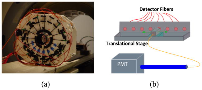
(a) The fiber optic interface. The 16-leg birdcage RF-coil is integrated into the interface, therefore, both optical and MRI measurements can be taken simultaneously. (b) The translational stage. A 1 mm single fiber was mounted on the translational stage to acquire data from the eight detector sites sequentially. The collected light is delivered to the shielded single PMT detection unit.
The picture of the shielded detection unit is shown in Figure 3.a. A head-on 8 mm diameter photocathode PMT (R7400U-20 Hamamatsu, Japan) was chosen as the detector. A 65 dB RF amplifier was used to amplify the output signal of the PMT. In FT, it is critical to separate the weak fluorescence signal from the excitation light leakage through the band-pass filters. When the excitation light is collimated perpendicular to the filter plane, the rejection band-pass filters eliminate the excitation light more efficiently (Hwang et al. 2005). To effectively eliminate the excitation light, two cascaded bandpass filters (830 nm, MK Photonics, Albuquerque, NM) were used. A collimation system was designed using aspheric lenses as shown in Figure 3.b. The lenses, filters and PMT were fixed in position by custom made plastic pieces, Figure 3.a. The PMT was placed at the focal point to achieve maximum signal strength. Eight 1 mm core diameter step-index fibers (Thorlabs, Newton, NJ) were utilized to collect the light from the phantom boundary. In order to collect data from eight detector positions using a single detection unit, a translational stage was used, Figure 2.b. All eight detector fibers were fixed on the translational stage, and a single collecting fiber was mounted on the moving platform of the stage, in order to collect signals sequentially from each detector fiber. The other end of the collecting fiber entered the collimation system through a waveguide to minimize the RF noise.
Figure 3.

a) The picture of the prototype PMT-based detection unit. The collimation system (1), incoming fiber (2), RF-amplifier (3) and PMT (4) are fixed in the unit. b) The schematic figure of the band-pass filters and collimation system. Two aspheric lenses are used to collimate the light coming out of the bundle and focus it on the PMT. Two cascaded band-pass filters (BP) are used to eliminate the excitation light.
The system was computer controlled. The data acquisition program was written in LabWindows CVI (National Instruments, Austin, Texas). Each source was turned on for approximately three seconds. Data were recorded at each detector position, with eight sources turning on and off sequentially by using a computer controlled fiber-optic switch. Thus, 64 amplitude and 64 phase values were acquired in a single measurement set within five minutes.
A 4T MRI system was used in this study. The birdcage coil was designed, tuned and matched specifically for the 4T magnetic field. High resolution spin echo T1-weighted MR images were acquired for the phantoms. The MRI acquisition parameters were 300 ms repetition time, 14 ms echo time, 90 degree flip-angle, 120 mm field of view, 4 mm slice-thickness and a matrix size of 256 × 256.
2.2 Image reconstruction
The light propagation through tissue can be written in the frequency domain as:
| (1) |
| (2) |
The subscript x, m and f indicate excitation, emission and fluorescence parameters. Φx(r, ω) and Φm(r, ω) (W·mm−2) are the fluence rates for the excitation and emission lights, respectively (Godavarty et al. 2005b, Lin et al. 2007, Patterson and Pogue 1994). The diffusion coefficient is defined by Dx,m=1/3(μax,m +μs′x,m). The reduced-scattering and absorption coefficients of the medium are represented by μs′x,m (mm−1) and μax,m (mm−1), respectively. The modulation angular frequency and the speed of light in the tissue are represented by ω and cn, respectively. The fluorescence parameters are the absorption coefficient due to the fluorophore, μaf (r), and the fluorescence lifetime, τ. Meanwhile, the quantum yield, η, is defined as the ratio of the number of photons emitted to the number of photons absorbed. The absorption coefficient of the fluorophore, μaf(r), is directly related to the concentration of the fluorophore by the formula μaf =2.3εC, where ε is the extinction coefficient of the fluorophore with the units of Molar−1·mm−1, and C is the concentration of the fluorophore.
The Robin boundary condition is used in our reconstruction and is given as
| (3) |
where n is the direction perpendicular to the boundary, and A is the boundary mismatch parameter. The latter accounts for the light reflection on the boundary surface which is determined by the Fresnel reflection (Haskell et al. 1994). The extrapolated-boundary condition is applied to model the position of the source (Haskell et al. 1994). A numerical solution of this partial differential equation (PDE) is applied in a nodal based finite element method (FEM) framework.
The error function for optimization can be written as:
| (4) |
Here, the index i represents the number of sources and j represents the number of detectors. is the measurement and Pij(μaf, τ) is the flux at the measured point, calculated by the forward solver from the spatial distribution of μaf and τ. There are fewer measurements than unknowns. Therefore, the unknowns, μaf and τ, are iteratively updated with a generalized inverse method, given by
| (5) |
where and X represents the unknown matrix of either μaf or τ. The dimension of X is N, which represents the number of nodes in the FEM mesh. The Jacobian matrix J is calculated with the adjoint method (Arridge 1999). When the structural a priori information is available, ‘Laplacian-type a priori’ is used to find the fluorophore concentration and lifetime for the inclusion and the background (Yalavarthy et al. 2007). The L-matrix can be written as
| (6) |
where Nr represents the number of nodes included in one region. Then the update equation can be expressed as:
| (7) |
During the reconstruction process, the fluorescence concentration map was initially reconstructed using only the amplitude measurements. However both amplitude and phase measurements were used in reconstructing the fluorescence lifetime map.
2.3 Phantom studies
Four phantom experiments were carried out to fully evaluate the performance of the system. Phantoms were prepared using agarose powder (OmniPur® Agarose, Lawrence, KS). Intralipid and Indian ink were added as the optical scattering and absorbing agents, respectively. Two different kinds of near infrared fluorophores were used in the experiment, Indocyanine Green, ICG (IC-Green, Akorn, Buffalo Grove, IL), and 3-3′ Diethylthiatricarbocyanine Iodide, DTTCI (Sigma-Aldrich Chemical Co., St. Louis, MO). Both fluorophores were excited by a 785 nm laser, and the emission light was collected using 830 nm bandpass filters, due to their similar excitation and emission spectra. However, the lifetime of ICG and DTTCI was different, 0.56 ns and 1.18 ns, respectively (Godavarty et al. 2005b). The ICG powder was first diluted in water, and later mixed with Intralipid and Indian ink to match the background optical properties. DTTCI is not water soluble, thus a small amount of dimethyl sulfoxide (DMSO, Sigma-Aldrich Chemical Co., St. Louis, MO) was used to dissolve the DTTCI. After that, Intralipid, Indian ink and water were added to match the background optical properties. The quantum efficiency of ICG in water is 0.016. We prepared ICG and DTTCI solutions, whose absorptions due to fluorophore (uaf) were both set to 0.01 mm−1. The emitted fluorescence intensity from both fluorophores was measured using the same excitation source. The signal strength of the DTTCI solution was 3.2 times higher than the ICG solution. Hence, the quantum efficiency was determined to be 0.051 for DTTCI in this study.
A calibration procedure was implemented to correct for the variation of each source and detector fiber. For this purpose an FT calibration phantom was made with a homogeneous ICG distribution. The optical properties of the calibration phantom were set to μa=0.01 mm−1, μs′=0.8 mm−1 and μaf=0.001 mm−1. A complete set of measurements were acquired from the calibration phantom. This step took into account the differences in transmission/alignment for each fiber and the data/model mismatch. Once calibrated, the data was used to reconstruct the fluorophore concentration and lifetime maps.
3. Results
3.1 System Noise Level
The noise level for the system was investigated in the first part of this study. The standard deviations (STD) of the amplitude and phase measurements with respect to the amplitude measurements are plotted in Figure 4. Based on the fitted curves shown as the dashed lines in Figure 4, the average standard deviation of the amplitude and phase were 0.02 dBm and 0.5 degrees at a signal level of −60 dBm. The standard deviation of both amplitude and phase measurements increased dramatically when the signal level was decreased. When the signal amplitude was decreased to approximately −90 dBm, the STD values increased to 1 dBm and 5 degrees, respectively. Accordingly, measurements taken at an amplitude below −90 dBm were excluded from the reconstructions discussed later. The −90 dBm threshold was chosen not only based on the STD values, but also on the number of measurements recorded above this level. As the fluorophore concentration decreased, the number of measurements above this threshold also decreased.
Figure 4.

The standard deviation (STD) of the amplitude and phase measurements, with respect to the amplitude measurements, is shown in a) and b), respectively.
3.2 Phantom Study I: Response Linearity
In this phantom study, a 38 mm diameter phantom was used. A 4.2 mm inner diameter thin wall glass tube filled with ICG was inserted into the phantom. The inclusion was located 9.5 mm away from the center. The homogeneous background optical properties are μa,m = 0.01 mm−1, and μs x,m = 1.0 mm−1. The axial MR image of the phantom is shown in Figure 5.a. Various ICG concentrations ranging from 86 nM to 1.17 μM were used to evaluate the response linearity of the system. Two phantoms were made to compare the system performance with and without background fluorescence. The first phantom had no fluorescence in the background, while the second phantom contained 34 nM background ICG (setting the absorption coefficient due to the fluorophore μaf = 0.001 mm−1 the). The ICG inclusions were reconstructed with and without the MRI structural a priori information.
Figure 5.

a) The axial MR image of the phantom. The ICG inclusion is held in the glass tube that is seen as a bright circle with a dark outline in the image. b) and c) The plot of the recovered mean ICG concentration with respect to true ICG concentration without and with background fluorescence, respectively. The circle and triangle dots represent the recovered values, with and without the structural a priori information, respectively. The least squares lines of best fit are the red dashed ones. The fitted equation is also shown in the Figure. The recovered ICG concentration shows a linear response with respect to true ICG concentration both with and without the structural a priori information. However, the true values are recovered only when structural a priori information is available.
Results (without background fluorescence)
The structure of the phantom was obtained from MRI, Figure 5.a. The recovered ICG concentration maps, with and without MRI structural a priori information, are shown in the first two columns of Figure 6. The recovered mean fluorophore concentration was linear with respect to the true concentration, both with and without structural a priori information, Figure 5.b. The correlation coefficient (r) was 0.998 for both fitted curves. However, the recovered ICG concentration was underestimated without MRI a priori information. The slope of the fitted curve increased from 0.095 to 1.02, indicating the accuracy of the recovered ICG concentration was improved considerably when MRI structural a priori information was utilized.
Figure 6.

The reconstructed ICG concentration maps for the first phantom study. When there is no ICG background, the reconstructed ICG concentration maps without (left column) and with (right column) structural a priori information from MRI are shown in the first and second columns. Meanwhile, when 34nM ICG is added to the background, the reconstructed ICG concentration maps without (left column) and with (right column) structural a priori information from MRI are shown in the third and forth columns. The color bars all have units of nM. The numbers on the right side present the true ICG concentration values.
Results (with background fluorescence)
The recovered ICG concentration maps, with and without MRI structural a priori information, are shown in the third and fourth columns of Figure 6. The recovered mean fluorophore concentration was linear with respect to the true concentration, both with and without structural a priori information, Figure 5.c. The correlation coefficient (r) was 0.994 and 0.984 for the fitted curves with and without MR information, respectively. Again, the recovered ICG concentration was underestimated without MRI a priori information. However, due to background fluorescence, the inclusion could not be resolved without MR a priori at very low concentrations (below contrast to background ratio of 2.5). This limit could have been lower if the inclusion size was increased. It is worth noting here that the 4.2 mm inclusion in the 38mm rat-sized phantom was very small, and thus difficult to resolve. On the other hand, when MRI structural a priori information was utilized, ICG concentration could be recovered within 10% error even for contrast to background ratio of 2.5.
Similar to the zero background case, the recovered mean fluorophore concentration was linear with respect to the true concentration, both with and without structural a priori information, Figure 5.c. The correlation coefficient (r) was 0.998 for both fitted curves. Again, the recovered ICG concentration is underestimated without MRI a priori information. The slope of the fitted curve increased from 0.095 to 1.02, indicating the accuracy of the recovered ICG concentration was improved considerably when MRI structural a priori information was utilized. The ICG concentration was underestimated without MRI information. This could have been caused by the reconstructed ICG size being spread over a larger area than the actual distribution.
3.3 Phantom Study II: Depth and Size Dependence
Due to the ill-posedness of the FT inverse problem, the reconstructed fluorescence concentration was expected to depend on the size and location of the inclusion. We evaluated this effect in this study. Furthermore, the reconstruction results were compared with and without the structural a priori information obtained from MRI. Again, a 38 mm diameter phantoms with homogeneous background optical property, μa,m = 0.01 mm−1 and μs x,m = 1.0 mm−1, were created. The size and location of the inclusion were varied, as listed in Table 1. However, the ICG concentration in the inclusion was kept the same, 669 nM, for all seven cases. Again, ICG concentration maps were reconstructed with and without structural MRI a priori information.
Table 1.
The recovered ICG concentrations for phantom study 2. The percentage error is shown in the parenthesis.
| Case # | Inclusion size (mm) | Offset (mm) | True ICG concentration (nM) | Recovered ICG concentration (nM) without MRI info | Recovered ICG concentration (nM) with MRI info |
|---|---|---|---|---|---|
| 1 | 4.2 | 9.5 | 669 | 68 (90%) | 686 (2.5%) |
| 2 | 3.2 | 9.5 | 669 | 35 (95%) | 666 (0.5%) |
| 3 | 3.2 | 14 | 669 | 184 (72%) | 630 (5.8%) |
| 4 | 2.4 | 14 | 669 | 54 (92%) | 629 (5.9%) |
| 5 | 4.2 | 7 | 669 | 42 (94%) | 697 (4.2%) |
Results
The recovered ICG concentrations with and without MRI a priori information for all the cases and the corresponding error values are listed in Table 1. Without MRI information, the recovered ICG concentration of a 4.2 mm inclusion had 94% error when the inclusion was located 7 mm from the center. As expected, the error was reduced to 90% when it was located 9.5 mm from the center. Similarly, the recovered ICG concentration error was 95% for the 3.2 mm inclusion located 9.5 mm from the center. The error reduced to 72% when the inclusion was located 14 mm from the center. In other words, the recovered ICG concentration is highly dependent on the depth of the inclusion without MRI a priori information.
Meanwhile, for an inclusion located 9.5 mm from the center, the error in the recovered ICG concentration was 95% for a 3.2 mm inclusion. The error reduced to 90% when the inclusion size was increased to 4.2 mm. Similarly, for an inclusion located 14 mm off the center, the error in the recovered ICG concentration was 92% for a 2.4 mm inclusion and reduced to 72% for a 3.2 mm inclusion. That is to say, the recovered ICG concentration is indeed highly dependent on the size of the inclusion without MRI a priori information.
As expected, the recovered ICG concentration is more accurate when the inclusion is closer to the surface and its size is larger. When MRI structural a priori information is used to guide the reconstruction, however, the ICG concentration is recovered within 6% error for all cases as shown in the last column in Table 1.
3.4 Phantom Study III: Multiple inclusions with various concentration and lifetime
Again, a phantom with similar background optical properties as the previous study was created. However this time, there were two 4.2 mm diameter inclusions located 9.5 mm away from the center of the phantom, and 90 degrees (13.4 mm) apart from each other. Two different cases were tested as listed in Table 2. Indeed, the quantum efficiency and extinction coefficient parameters were different for both fluorophores. Therefore, the fluorophore concentration maps are replaced by the quantum yield, ημaf, maps. While both objects had similar fluorescence quantum yield in the first case, the DTTCI had about 4 times higher quantum yield than ICG in the second case.
Table 2.
The recovered fluorophore intensity and lifetime for phantom study 3. The percentage error is shown in the parenthesis.
| Case # | Obj # | True Yield ημaf (×10−5) | True Lifetime (ns) | Recovered Yield ημaf (×10−5 mm−1) | Recovered Lifetime (ns) | ||
|---|---|---|---|---|---|---|---|
|
| |||||||
| No MRI | With MRI | No MRI | With MRI | ||||
| 1 | 1 | 25.6 | 1.12 | 5.4 (80%) | 25 (4.0%) | 1.53 (37%) | 1.19 (6.3%) |
| 2 | 32.0 | 0.56 | 5.5 (83%) | 34 (6.2%) | 0.77 (38%) | 0.53 (5.4%) | |
| 2 | 1 | 51.2 | 1.12 | 8.5 (83%) | 52 (1.6%) | 1.31 (17%) | 1.14 (1.8%) |
| 2 | 16.0 | 0.56 | 2.5 (84%) | 18 (12%) | 0.63 (13%) | 0.51 (8.9%) | |
Results
The recovered fluorophore quantum yield (ημaf) and lifetime parameters with and without MRI a priori information for all the cases together with the corresponding error values are listed in Table 2. The MR image of the phantom is shown in the first row of Figure 8. The second and third rows are the reconstructed fluorescence quantum yield and lifetime maps for the first case, while the fourth and fifth rows are for the second case. The left column shows the quantum yield and lifetime maps are shown in the right column. For both cases, the accuracy of the recovered fluorophore quantum yield was significantly improved when MR a priori information was used as listed in Table 2. Similarly, the recovered lifetime was also significantly improved. Please note that although concentrations of both ICG and DTTCI were different for each case, the lifetime parameter was successfully recovered, independent from the fluorescence quantum yield parameter.
Figure 8.

The results for the third phantom study. The first row shows the MR image of the phantom. The second and third rows show the reconstructed ημaf maps, without and with MRI a priori information. Meanwhile, the fourth and fifth rows present the lifetime maps reconstructed without and with MRI a priori information.
3.5 Phantom Study IV: In the presence of background fluorescence
An important aspect in fluorescence tomography studies is the contribution of background fluorescence, as there is likely to be residual fluorescence and/or auto fluorescence from the tissue surrounding the target. In this last phantom study, the ability of the system to recover the inclusion properties in the presence of the background fluorescence was investigated. Furthermore, the inclusion had lifetime contrast in addition to concentration contrast. Lifetime can only be resolved using time-resolved measurements. 34 nM ICG was added to the background, setting the absorption coefficient due to the fluorophore to μaf = 0.001 mm−1. An 8.8 mm diameter inclusion filled with 1μM DTTCI was located 9.5 mm away from the center. Again, fluorophore quantum yield maps were used instead of concentration maps due to the existence of two distinct fluorophores.
Results
The inclusion could be clearly localized on the quantum yield map in the presence of the background fluorescence, even without MRI structural a priori information, as shown in Figure 9. The recovered value for DTTCI inclusion and ICG background was 38.4 mm−1 (56% error) and 0.8 mm−1 (50% error), respectively. On the other hand, when MRI a priori information was used, the recovered value for DTTCI inclusion and ICG background was 49 mm−1 (8% error) and 1.7 mm−1 (5% error), as shown in Figure 9. The reconstructed lifetime maps are shown in the second column. The DTTCI inclusion could be localized on the lifetime images without a priori information. However, the error in the recovered DTTCI lifetime was 50%. When MRI structural a priori information was available, DTTCI’s longer lifetime was accurately recovered with 2% error.
Figure 9.

The results for the fourth phantom study. The left column shows the reconstructed ημaf maps (mm−1) without and with MR a priori information. Meanwhile, the right column presents the lifetime maps reconstructed without and with MR a priori information.
4. Conclusion and Discussion
Fluorescence tomography has become an essential in vivo small animal imaging tool in recent years. Commercially available FT systems have enabled widespread adoption of this technique. Despite its high sensitivity, FT is a low spatial resolution molecular imaging modality because of the strong light scattering in tissue. This also makes the inverse problem of FT severely ill-posed. An ideal FT system should not only allow visualization of the fluorophore distribution in tissue, but also provide quantitatively accurate concentration values. Quantitative accuracy is an important factor for many practical applications of FT. This is because there is no molecular agent that has perfect specificity, often accumulating in benign lesions in smaller amounts (Bremer et al. 2001). To be able to differentiate malignant and benign lesions, the reconstructed fluorescence concentration value should discern different fluorescence concentrations and be independent of the size and location of the lesion. A stand-alone FT system, unfortunately, would not correctly differentiate between a small malignant lesion buried deep in the tissue, and a large benign lesion located close to the surface of the tissue. We demonstrated this in the second phantom study.
In order to address the need for quantitative FT imaging, we built a hybrid MR-FT system. The main objective is to utilize high resolution MR images to constrain and guide the FT reconstruction algorithm to obtain quantitative fluorescence parameters. Because this system uses an MRI, an optical-fiber-based contact system was needed so that all the electronics could be placed far away from the high magnetic field of the MRI bore. This significantly limits the number of sampling points compared with CCD-based small-animal FT systems. The rationale is that MRI provides excellent spatial resolution and soft tissue contrast; therefore, the region of interest is obtained from MRI. Subsequently, the limited number of fluorescence measurements can be used to obtain quantitative fluorescence parameters with the guidance of anatomical priors.
In the literature, nearly all of the FT systems focus on the measurement of the fluorophore concentration alone. Recently, there has been a great interest in fluorescence lifetime tomography. Fluorescence lifetime holds promise in investigating the micro-environment of a lesion as demonstrated in fluorescence lifetime imaging microscopy (Cubeddu and et al. 2002). For example, using a planar imaging system, Erten et al. demonstrated that fluorescence intensity and lifetime images enhance the sensitivity of MRI in tumor detection (Erten et al. 2010). However, they also mention that challenges remain since varying the tissue thickness modifies the apparent lifetime and fluorophore intensity. This conclusion also supports the importance of our tomographic imaging approach that can provide spatially resolved lifetime parameters. In addition, one advantage of the the fluorescence lifetime parameter is that even when a small amount of fluorophore is accumulated, the change in lifetime can still be detected, as we showed in the third phantom study. Despite the great potential of lifetime imaging, however, it has not been widely utilized for in vivo imaging. A few studies have reported the fluorescence lifetime measurement using stand-alone time-dependent FT systems (Bloch et al. 2005, Culver et al. 2007, Gao et al. 2010, Godavarty et al. 2005b, Kumar et al. 2008, Nothdurft et al. 2009, Soloviev V Y and Arridge 2007). A time-dependent FT system is more complicated than the more commonly used continuous wave system. Therefore, it is non-trivial to build a time-resolved FT system that is compatible with MRI. Our hybrid MR-FT system is the first of its kind: a time-resolved multi-modality FT system that can resolve both fluorescence concentration and lifetime parameters.
The optical background was assumed to be homogeneous to simplify the problem in the current study. However, in real life the background can be highly heterogeneous. We have shown in previous studies that the optical background heterogeneity can be corrected for, by taking diffuse optical tomography (DOT) measurements along with FT measurements (Lin et al. 2010, Lin et al. 2007, Lin et al. 2009). Integrating a frequency domain DOT system into the current FT-MRI system is under development. It is expected that such a system can provide truly quantitative fluorescence parameters in heterogeneous tissues. In reality, there are several other source of errors may affect quantitative accuracy of FT such as source-detector probe coupling to the tissue surface, source-detector position uncertainty and errors in delineating medium boundary from the MR images. The dependency of the MR anatomical information accuracy for FT reconstruction can also be a source of error, which we have discussed in our previous publication (Lin et al. 2009). Nevertheless, the improvement from anatomical image guidance is still very significant although experiment uncertainties are inevitable. Finally, modeling errors might introduce errors in the reconstruction results, especially due to the presence of low scattering regions in tissue. Accordingly, we are currently working on adapting Radiative Transfer Equation for our reconstruction algorithm.
As mention in the previous sections, only a single PMT detection unit is used in this study. We are currently extending this FT system to be able to collect data from all detector sites simultaneously, which would increase the temporal resolution of the system nearly eight times. Having temporal resolution of 30 seconds, this new system would allow us to acquire dynamic FT measurements. In conclusion, we have demonstrated the feasibility of a hybrid fluorescence tomography and MR system for small animal imaging. The FT system utilizes a PMT and is able to measure frequency domain measurements with high sensitivity.
Figure 7.

The results for the second phantom study. The first column is the MRI images of the phantoms. Each case has an inclusion with a different location and size. The reconstructed ICG concentration maps, without and with structural a priori information from MRI, are shown in the second and third columns, respectively. The recovered ICG concentration value drastically depends on the size and location of the inclusion without any a priori information. However, the true concentration value can be recovered for all seven cases when MRI structural a priori information is used. The color bars all have the units of nM.
Table 3.
The recovered fluorophore intensity and lifetime for phantom study 4. The percentage error is shown in the parenthesis.
| True Yield ημaf (×10−5) | True ICG Lifetime (ns) | Recovered Yield ημaf (×10−5 mm−1) | Recovered Lifetime (ns) | |||
|---|---|---|---|---|---|---|
|
| ||||||
| No MRI | With MRI | No MRI | With MRI | |||
| Inclusion | 51.2 | 1.12 | 22.3 (56%) | 49 (8%) | 1.66 (50%) | 1.1 (2%) |
| Background | 1.6 | 0.56 | 0.8 (50%) | 1.7 (5%) | 0.6 (7%) | 0.59 (5%) |
Acknowledgments
This research is supported in part by the National Institutes of Health (NIH) grants R01EB008716, R21/33 CA120175, R21 CA121568, R01CA142989 and Suzan G. Komen Foundation grant KG101442. It was also supported in part by the World Class University Program through the National Research Foundation of Korea funded by the Ministry of Education, Science and Technology, Republic of Korea (grant no. R31-20004-(ON)).
References
- Ale A, Schulz RB, Sarantopoulos A, Ntziachristos V. Imaging performance of a hybrid x-ray computed tomography-fluorescence molecular tomography system using priors. Medical Physics. 2010;37:1976–1986. doi: 10.1118/1.3368603. [DOI] [PubMed] [Google Scholar]
- Arridge SR. Optical tomography in medical imaging. Inverse Problems. 1999;15:R41–R93. [Google Scholar]
- Bloch S, Lesage F, McIntosh L, Gandjbakhche A, Liang K, Achilefu S. Whole-body fluorescence lifetime imaging of a tumor-targeted near-infrared molecular probe in mice. Journal of Biomedical Optics. 2005;10:054003. doi: 10.1117/1.2070148. [DOI] [PubMed] [Google Scholar]
- Bremer C. Optical methods. Handbook of Experimental Pharmacology. 2008;(185 Pt 2):3–12. doi: 10.1007/978-3-540-77496-9_1. [DOI] [PubMed] [Google Scholar]
- Bremer C, Bredow S, Mahmood U, Weissleder R, Tung CH. Optical imaging of matrix metalloproteinase-2 activity in tumors: feasibility study in a mouse model. Radiology. 2001;221:523–529. doi: 10.1148/radiol.2212010368. [DOI] [PubMed] [Google Scholar]
- Bremer C, Ntziachristos V, Weissleder R. Optical-based molecular imaging: contrast agents and potential medical applications. European radiology. 2003;13:231–243. doi: 10.1007/s00330-002-1610-0. [DOI] [PubMed] [Google Scholar]
- Corlu A, Choe R, Durduran T, Rosen MA, Schweiger M, Arridge SR, Schnall MD, Yodh AG. Three-dimensional in vivo fluorescence diffuse optical tomography of breast cancer in humans. Optics Express. 2007;15:6696. doi: 10.1364/oe.15.006696. [DOI] [PubMed] [Google Scholar]
- Cubeddu R, et al. Time-resolved fluorescence imaging in biology and medicine. Journal of Physics D: Applied Physics. 2002;35:R61. [Google Scholar]
- Culver JP, Patwardhan S, Nothdurft R, Achilefu S. Quantitative fluorescence lifetime tomography for small animals. 2007. [DOI] [PubMed] [Google Scholar]
- Davis SC, Pogue BW, Springett R, Leussler C, Mazurkewitz P, Tuttle SB, Gibbs-Strauss SL, Jiang SS, Dehghani H, Paulsen KD. Magnetic resonance-coupled fluorescence tomography scanner for molecular imaging of tissue. The Review of scientific instruments. 2008;79:064302. doi: 10.1063/1.2919131. [DOI] [PMC free article] [PubMed] [Google Scholar]
- Erten A, Hall D, Hoh C, Cao HST, Kaushal S, Esener S, Hoffman RM, Bouvet M, Chen J, Kesari S, Makale M. Enhancing magnetic resonance imaging tumor detection with fluorescence intensity and lifetime imaging. Journal of Biomedical Optics. 2010;15:066012–6. doi: 10.1117/1.3509111. [DOI] [PMC free article] [PubMed] [Google Scholar]
- Frangioni JV. In vivo near-infrared fluorescence imaging. Current Opinion in Chemical Biology. 2003;7:626. doi: 10.1016/j.cbpa.2003.08.007. [DOI] [PubMed] [Google Scholar]
- Gao F, Li J, Zhang L, Poulet P, Zhao H, Yamada Y. Simultaneous fluorescence yield and lifetime tomography from time-resolved transmittances of small-animal-sized phantom. Appl Opt. 2010;49:3163–3172. doi: 10.1364/AO.49.003163. [DOI] [PubMed] [Google Scholar]
- Ge J, Erickson SJ, Godavarty A. Fluorescence tomographic imaging using a handheld-probe-based optical imager: extensive phantom studies. Appl Opt. 2009;48:6408–6416. doi: 10.1364/AO.48.006408. [DOI] [PMC free article] [PubMed] [Google Scholar]
- Godavarty A, Eppstein MJ, Zhang C, Sevick-Muraca EM. Detection of single and multiple targets in tissue phantoms with fluorescence-enhanced optical imaging: feasibility study. Radiology. 2005a;235:148–154. doi: 10.1148/radiol.2343031725. [DOI] [PubMed] [Google Scholar]
- Godavarty A, Sevick-Muraca EM, Eppstein MJ. Three-dimensional fluorescence lifetime tomography. Medical physics. 2005b;32:992–1000. doi: 10.1118/1.1861160. [DOI] [PubMed] [Google Scholar]
- Haskell RC, Svaasand LO, Tsay T, Feng TC, McAdams MS, Tromberg BJ. Boundary conditions for the diffusion equation in radiative transfer. Journal of the Optical Society of America A, Optics, image science, and vision. 1994;11:2727. doi: 10.1364/josaa.11.002727. [DOI] [PubMed] [Google Scholar]
- Hoshino K, Ly HQ, Frangioni JV, Hajjar RJ. In Vivo Tracking in Cardiac Stem Cell-Based Therapy. Progress in Cardiovascular Diseases. 2007;49:414–420. doi: 10.1016/j.pcad.2007.02.005. [DOI] [PubMed] [Google Scholar]
- Hwang K, Houston JP, Rasmussen JC, Joshi A, Ke S, Li C, Sevick-Muraca EM. Improved excitation light rejection enhances small-animal fluorescent optical imaging. Molecular imaging: official journal of the Society for Molecular Imaging. 2005;4:194–204. doi: 10.1162/15353500200505142. [DOI] [PubMed] [Google Scholar]
- Kepshire D, Davis SC, Dehghani H, Paulsen KD, Pogue BW. Fluorescence tomography characterization for sub-surface imaging with protoporphyrin IX. Optics express. 2008;16:8581–8593. doi: 10.1364/oe.16.008581. [DOI] [PMC free article] [PubMed] [Google Scholar]
- Kepshire D, Mincu N, Hutchins M, Gruber J, Dehghani H, Hypnarowski J, Leblond F, Khayat M, Pogue BW. A microcomputed tomography guided fluorescence tomography system for small animal molecular imaging. The Review of scientific instruments. 2009;80:043701. doi: 10.1063/1.3109903. [DOI] [PMC free article] [PubMed] [Google Scholar]
- Kepshire DS, Davis SC, Dehghani H, Paulsen KD, Pogue BW. Subsurface diffuse optical tomography can localize absorber and fluorescent objects but recovered image sensitivity is nonlinear with depth. Applied Optics. 2007;46:1669. doi: 10.1364/ao.46.001669. [DOI] [PubMed] [Google Scholar]
- Koenig A, Herve L, Josserand V, Berger M, Boutet J, Da Silva A, Dinten JM, Peltie P, Coll JL, Rizo P. In vivo mice lung tumor follow-up with fluorescence diffuse optical tomography. Journal of Biomedical Optics. 2008;13:011008. doi: 10.1117/1.2884505. [DOI] [PubMed] [Google Scholar]
- Kumar ATN, Raymond SB, Dunn AK, Bacskai BJ, Boas DA. A Time Domain Fluorescence Tomography System for Small Animal Imaging. Medical Imaging, IEEE Transactions on. 2008;27:1152–1163. doi: 10.1109/TMI.2008.918341. [DOI] [PMC free article] [PubMed] [Google Scholar]
- Leblond F, Davis SC, Valdés PA, Pogue BW. Pre-clinical whole-body fluorescence imaging: Review of instruments, methods and applications. Journal of Photochemistry and Photobiology B: Biology. 2010;98:77–94. doi: 10.1016/j.jphotobiol.2009.11.007. [DOI] [PMC free article] [PubMed] [Google Scholar]
- Lin Y, Barber WC, Iwanczyk JS, Roeck W, Nalcioglu O, Gulsen G. Quantitative fluorescence tomography using a combined tri-modality FT/DOT/XCT system. Opt Express. 2010;18:7835–7850. doi: 10.1364/OE.18.007835. [DOI] [PMC free article] [PubMed] [Google Scholar]
- Lin Y, Gao H, Nalcioglu O, Gulsen G. Fluorescence diffuse optical tomography with functional and anatomical a priori information: feasibility study. Physics in Medicine and Biology. 2007;52:5569–5585. doi: 10.1088/0031-9155/52/18/007. [DOI] [PubMed] [Google Scholar]
- Lin Y, Yan H, Nalcioglu O, Gulsen G. Quantitative fluorescence tomography with functional and structural a priori information. Appl Opt. 2009;48:1328–36. doi: 10.1364/ao.48.001328. [DOI] [PMC free article] [PubMed] [Google Scholar]
- Milstein AB, Oh S, Webb KJ, Bouman CA, Zhang Q, Boas DA, Millane RP. Fluorescence optical diffusion tomography. Applied Optics. 2003;42:3081–3094. doi: 10.1364/ao.42.003081. [DOI] [PubMed] [Google Scholar]
- Milstein AB, Stott JJ, Oh S, Boas DA, Millane RP, Bouman CA, Webb KJ. Fluorescence optical diffusion tomography using multiple-frequency data. Journal of the Optical Society of America A, Optics, image science, and vision. 2004;21:1035–1049. doi: 10.1364/josaa.21.001035. [DOI] [PubMed] [Google Scholar]
- Nothdurft RE, Patwardhan SV, Akers W, Ye Y, Achilefu S, Culver JP. In vivo fluorescence lifetime tomography. Journal of Biomedical Optics. 2009;14:024004. doi: 10.1117/1.3086607. [DOI] [PubMed] [Google Scholar]
- Ntziachristos V. Fluorescence molecular imaging. Annual Review of Biomedical Engineering. 2006;8:1–33. doi: 10.1146/annurev.bioeng.8.061505.095831. [DOI] [PubMed] [Google Scholar]
- Ntziachristos V, Bremer C, Weissleder R. Fluorescence imaging with near-infrared light: new technological advances that enable in vivo molecular imaging. European radiology. 2003;13:195–208. doi: 10.1007/s00330-002-1524-x. [DOI] [PubMed] [Google Scholar]
- Patterson MS, Pogue BW. Mathematical model for time-resolved and frequency-domain fluorescence spectroscopy in biological tissues. Applied Optics. 1994:33. doi: 10.1364/AO.33.001963. [DOI] [PubMed] [Google Scholar]
- Sevick-Muraca EM, Rasmussen JC. Molecular imaging with optics: primer and case for near-infrared fluorescence techniques in personalized medicine. Journal of Biomedical Optics. 2008;13:041303. doi: 10.1117/1.2953185. [DOI] [PMC free article] [PubMed] [Google Scholar]
- Soloviev VY, TKBMJEDSNMAAFPMW, Arridge SR. Fluorescence lifetime imaging by using time gated data acquisition. Appl Opt. 2007;46:7384. doi: 10.1364/ao.46.007384. [DOI] [PubMed] [Google Scholar]
- Tan Y, Jiang H. Diffuse optical tomography guided quantitative fluorescence molecular tomography. Applied Optics. 2008;47:2011–2016. doi: 10.1364/ao.47.002011. [DOI] [PubMed] [Google Scholar]
- Venugopal V, Chen J, Lesage F, Intes X. Full-field time-resolved fluorescence tomography of small animals. Opt Lett. 2010;35:3189–3191. doi: 10.1364/OL.35.003189. [DOI] [PubMed] [Google Scholar]
- Yalavarthy PK, Pogue BW, Dehghani H, Carpenter CM, Jiang H, Paulsen KD. Structural information within regularization matrices improves near infrared diffuse optical tomography. Optics Express. 2007;15:8043. doi: 10.1364/oe.15.008043. [DOI] [PubMed] [Google Scholar]
- Zhang X, Badea C, Jacob M, Johnson GA. Development of a noncontact 3-D fluorescence tomography system for small animal in vivo imaging. Proceedings - Society of Photo-Optical Instrumentation Engineers. 2009;7191:nihpa106691. doi: 10.1117/12.808199. [DOI] [PMC free article] [PubMed] [Google Scholar]