Evaluating, Comparing, and Interpreting Protein Domain Hierarchies

Abstract

Arranging protein domain sequences hierarchically into evolutionarily divergent subgroups is important for investigating evolutionary history, for speeding up web-based similarity searches, for identifying sequence determinants of protein function, and for genome annotation. However, whether or not a particular hierarchy is optimal is often unclear, and independently constructed hierarchies for the same domain can often differ significantly. This article describes methods for statistically evaluating specific aspects of a hierarchy, for probing the criteria underlying its construction and for direct comparisons between hierarchies. Information theoretical notions are used to quantify the contributions of specific hierarchical features to the underlying statistical model. Such features include subhierarchies, sequence subgroups, individual sequences, and subgroup-associated signature patterns. Underlying properties are graphically displayed in plots of each specific feature's contributions, in heat maps of pattern residue conservation, in “contrast alignments,” and through cross-mapping of subgroups between hierarchies. Together, these approaches provide a deeper understanding of protein domain functional divergence, reveal uncertainties caused by inconsistent patterns of sequence conservation, and help resolve conflicts between competing hierarchies.

1. Introduction

The manner in which evolutionarily related protein domains have functionally diverged from an ancient common ancestor is typically investigated by constructing a phylogenetic tree (Felsenstein, 2004). Such trees rely on sequence similarity to model the hierarchical relationships between proteins conserving that domain. Each leaf node in the tree corresponds to an actual sequence, each internal node corresponds to a hypothetical ancestral sequence, and each subtree typically corresponds to functionally related proteins that presumably share similar biochemical and biophysical properties.

However, given that many classes of protein domains contain thousands of sequences, modeling protein functional divergence in this way is problematic for the following reasons. (i) Finding the optimal tree is extremely challenging computationally. (ii) The optimal tree is unlikely to correspond to the evolutionarily correct tree because of the typically very large number of nearly equally likely alternative trees. (iii) It is difficult to justify such high-complexity models. (iv) It is unclear what biological insight such large trees provide. (v) Such a tree fails to reveal those amino acid residues likely responsible for the biological properties associated with specific divergent functions.

An alternative approach to constructing large sequence-level trees is to model a set of related protein domains as hierarchically arranged clusters of biologically similar subgroups. This approach is used, for example, in the construction of the National Center for Biotechnology Information (NCBI) Conserved Domain Database (CDD) (Marchler-Bauer et al., 2003, 2011). A basic assumption underlying this approach is that ancient protein domains have diverged into functionally related subgroups, each of which conserves similar biologically relevant properties. These conserved properties are presumably reflected at the sequence level as conserved residue signatures distinctive of each divergent subgroup.

NCBI conserved domain hierarchies are created through manual curation in the light of sequence alignments, phylogenetic trees, structural data, and the published literature—though we recently developed a heuristically based approach to generate such hierarchies automatically (Neuwald et al., 2012). Moreover, our recent article in this journal (Neuwald, 2014) describes a procedure for obtaining an optimal or nearly optimal domain hierarchy via Bayesian Markov chain Monte Carlo (MCMC) sampling (Liu, 2008). This approach takes as input a multiple alignment of, in principle, every available sequence for a given protein domain. It searches for an optimal hierarchy by probabilistically adding and removing nodes, moving nodes up and down the hierarchy, moving sequences between nodes, and redefining the residue patterns distinctive of each divergent subgroup. MCMC sampling is necessary because often the number of possible hierarchies and the number of the associated sequence and pattern assignments are astronomical and thus cannot be enumerated exhaustively.

The nature of a hierarchy for a given domain depends, of course, on the individual constructing it and on the methods used. This raises the question of whether or not a given hierarchical configuration is optimal or nearly so. Moreover, even when a hierarchy is optimal, inherent statistical uncertainties will remain, thereby raising questions regarding the level of support for various features of the hierarchy: With what confidence may a specific sequence be assigned to a specific subgroup? Do all of the sequences assigned to a specific subgroup share the features of that subgroup in roughly equal measure or is there considerable variability between sequences? Which signature residues most distinguish a functionally divergent subgroup from closely related subgroups? Which subgroups have most strikingly diverged in sequence (and presumably in function)? Do certain sequences have unusual features, such as conserved residues characteristic of a subgroup, but not of an ancestral supergroup? (Such inconsistent features may occur in proteins that, for example, are related to and conserve the biochemical properties of a specific subgroup within an enzyme class but that lack the catalytic activity characteristic of that class.) Given two independently derived hierarchies, what characteristics do they share and in what respect do they differ and why? Is one hierarchy more correct than another, or do they merely provide different perspectives and thus reveal different aspects of underlying biological properties? (For example, given the nature of biology, an ensemble of nearly optimal hierarchical configurations may be of approximately equal biological relevance.) This article describes statistically based approaches that can address such questions.

2. Background

The statistical model for protein domain hierarchies is described in a previous article (Neuwald, 2014) and thus is merely summarized here. Such a model is illustrated in Figure 1, as follows: Figure 1A shows a protein domain hierarchy consisting of N = 12 nodes and of M = 12 functionally divergent subgroups, each of which corresponds to a subtree. (We also allow, though not here, N ≠ M, which corresponds to a graph other than a tree.) Figure 1B shows how the divergent sequence constraints for each of these subgroups are quantified. This involves defining, for each subtree, a tri-partitioning of the nodes in the hierarchy into (i) the subtree itself (termed the “foreground”), (ii) other, closely related nodes (termed the “background”), and (iii) the remaining (nonparticipating) nodes. More specifically, the background corresponds to the rest of the subtree rooted at the parent of the foreground subtree for each tri-partition. Each tri-partition is also termed a “contrast alignment” because it reveals how the foreground aligned sequences diverge from or contrast with the background sequences. The background for the main tree (rooted at node 1 in Fig. 1A) is based on random sequences. The collection of such hierarchically arranged contrast alignments (one for each subtree within the tree) identifies the distinguishing patterns (illustrated in Fig. 1C) associated with each functionally divergent subgroup within the protein class.

FIG. 1.

(A) Hypothetical protein domain hierarchy. The hierarchy consists of N = 12 sequence subsets (each corresponding to a node; indexed as 1 ≤ z ≤ N) and M = 12 divergent subgroups (each corresponding to a subtree; indexed as 1 ≤ h ≤ M). The tree is colored to highlight subgroup h = 4 (the blue subtree), which is presumed to have diverged most recently from the rest of subgroup h = 2 (maroon nodes). (B) Schematic of a tri-partitioned alignment corresponding to subgroup h = 4 in (A). Such a tri-partition (also called a contrast alignment) is represented mathematically as 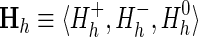, where each sequence subset (corresponding to each node) is assigned to a foreground partition (), a background partition (), or a nonparticipating partition (). The sequences in these partitions are represented by blue, maroon, and gray horizontal bars, respectively. The corresponding nodes in the tree in (A) are colored similarly. Partitioning is based on the conservation of foreground residues (blue vertical bars) that most diverge from (or contrast with) the background residue compositions at those positions (white vertical bars). Red vertical bar heights quantify the degree of divergence. (C) Hypothetical residue sets conserved at discriminating positions in the contrast alignment. The residue set at position j in contrast alignment h is represented mathematically by A_h,j with A_h,j =  at nondiscriminating positions.

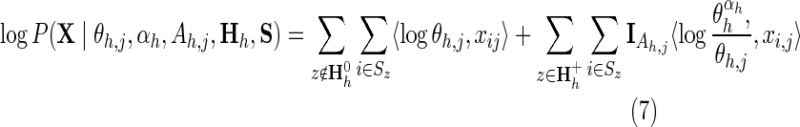
The probability distribution associated with this hierarchical model is defined (logarithmically) by

where X is an n × k matrix representing an alignment of k columns and n sequences; x_i,j is a bitwise vector specifying the residue observed in the ith sequence and the jth column; Θ is an h × j matrix of vectors representing the position-specific amino acid compositions for each of the foreground and background partitions; at nonpattern positions, the vector θ_j corresponds to the overall (foreground and background) composition; 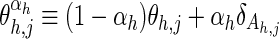models the foreground composition at pattern positions, where is the background “functional” and “nonfunctional” residue frequency vector for column j, where the parameter α_h specifies the expected background “contamination” at pattern positions in the foreground, and where is a bit vector specifying the pattern residues at position j for subgroup h; A_h,j specifies the set of functional residues at that position (as in Fig. 1C); denotes the hierarchically configured tri-partitioning of the node indices 1 ≤ z ≤ N (as in Fig. 1B); S is an array of N disjoint sets, each of which indicates the distinct set of sequences assigned to that node in the hierarchy; is an indicator variable equal to 0 when A_h,j =  and to 1 when A_h,j ≠ . The inner product of two vectors is denoted by . The third through seventh terms in Equation 1 correspond to the logarithm of the product of the prior probabilities, as defined in Neuwald (2014).

3. Comparing and Evaluating Hierarchies

This section first describes methods for comparing the relationships between corresponding, node-associated subgroups within two different hierarchies. Next, it describes a statistical and information theoretical measure of the quality of a given hierarchy. Finally, it describes a way to measure the contributions of subhierarchies, of node- and subtree-associated sequence subgroups, of individual sequences, and of signature patterns to the overall quality of a hierarchy.

3.1. Comparing two hierarchies

To compare two hierarchies, one must first determine the correspondence between the nodes in each hierarchy. This involves two procedural steps: (i) identifying corresponding (or roughly corresponding) nodes so that nodes in one hierarchy can be mapped to the other, and (ii) rearranging one of the hierarchies to best resemble the other hierarchy.

3.1.1. Mapping one hierarchy to another

This first step requires, for each node z within each tree, a set of identifiers, S_z, representing the sequence set associated with that node. For each hierarchy, we also require that (i) 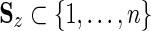, where n is the number of sequences in the input alignment used to construct both hierarchies; (ii) z ≠ z′ → S_z∩S_z′ = ; and (iii), 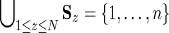where N is the number of nodes in the hierarchy. We likewise define for each subtree within each hierarchy a set of sequence identifiers representing the sequences associated with the subtree rooted at node z. We define as corresponding those pairs of nodes or subtrees, one from each hierarchy, with ≥90% overlap in their sequence sets; as roughly corresponding such pairs with >50% but <90% overlap; and as noncorresponding the remaining nodes. We represent sequence sets using a previously described data structure (Neuwald and Green, 1994) facilitating efficient bitwise set operations.

3.1.2. Rearranging nodes in one hierarchy to best resemble another

This second step is required because there are number of ways to arrange the nodes within a tree of N nodes, where d_z is the number of children of the zth node. Thus, even for the simple tree shown in Figure 1, there are 576 ways to arrange the nodes. To easily compare hierarchies, the nodes in each hierarchy are arranged similarly, so as to best reveal which nodes and subtrees correspond. This is accomplished by recursively sorting the child subtrees at each level of one of the hierarchies (starting from the root) to be consistent with the ordering of the corresponding nodes and subtrees in the other hierarchy.

3.2. Measures of hierarchy quality

As a measure of hierarchy quality, we utilize the information theoretical notion of relative entropy (Cover and Thomas, 1991):

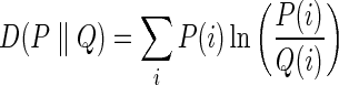which measures the expected additional descriptive length required to encode information using the (wrong) probability distribution Q, instead of the true distribution P, and which is equivalent to the expected log likelihood ratio of P to Q. Applying this to Equation 1, we obtain:

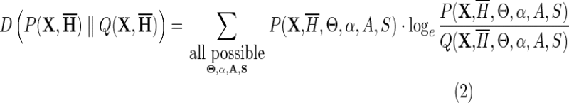where 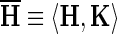is a 2-tuple that associates with each node z in the hierarchy H a consensus sequence, denoted as K_z, and where is the probability associated with a null hierarchy ^ØH where all of the foreground sequence sets, the S_z, are assigned to the background partition for all subgroups, h, that is, where 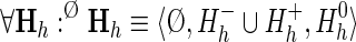. The vector K of consensus sequences is required to define the nature of each node; without this, for example, three child nodes attached to a common parent node would be indistinguishable. Each residue r_j at pattern position j in sequence K_z helps define the hierarchy by requiring that r_j be a member of that pattern's residue set. Equation 2 quantifies how well the data support the hierarchy and avoid over fitting by summing over variable parameters. From the perspective of information theory, it calculates the information gained (in nats) using the specified hierarchy instead of the null hierarchy, which is otherwise similar except that it treats the sequence data, X, as lacking discriminating patterns. Conversely, it measures the expected additional descriptive length required to encode the domain hierarchy using this null distribution Q, instead of the distribution P. Therefore, the more closely P models the discriminating patterns present in alignment X, the more Equation 2 will increase.

Equation 2 cannot be computed directly, though it could be estimated as the corresponding expected log-likelihood ratio (LLR) using the mcBPPS sampler (Neuwald, 2011), which by design keeps constant during sampling. This involves continuing to sample values for the LLR after convergence (proportional to 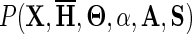) and taking the average. As a faster, less accurate alternative, we can simply use the value of the LLR corresponding to the maximum a posteriori probability (MAP) as an upper bound on Equation 2. This upper bound appears to be conservative based on the empirical observation that, after convergence, the average of the mcBPPS-sampled values is typically only slightly lower (roughly by no more than 15% less) than the LLR for the (presumed) MAP. The MAP, which corresponds to the maximum LLR (denoted here as LLR_MAP), is the value to which the sampler (with simulated annealing) tends to converge, though this is not guaranteed. As illustrated by Neuwald (2014), however, obtaining the same maximum LLR in multiple sampling runs using distinct random seeds suggests that a nearly optimal hierarchy is typically found. Of course, when comparing such MAP-associated LLRs for distinct hierarchies, it is essential that the same input alignment be used throughout. Note that if discriminating patterns are eliminated from an input alignment by randomly shuffling residues within each column, then both the LLR_MAP and Equation 2 will be zero, as expected.

3.3. Contributions of a specific subtree, sub-subtree, or subhierarchy

The contribution of the hth subtree to the quality of a given hierarchy is defined as the expected subLLR (i.e., that component of Eq. 2) corresponding to the contrast alignment for that subtree. Here, however, we will simply compute the contribution of the hth contrast alignment to the LLR_MAP, which we represent as subLLR(h). Using the MAP parameter settings, this is straightforward to compute by summing Equation 1 only over this one h, rather than over all h:

Less straightforward is assessing how much each node or sub-subtree within subgroup h contributes to the subLLR(h). Such sub-subLLRs provide an indication of how well each subgroup (either a node or a subtree) matches the distinguishing characteristics of each supergroup (i.e., each internal node) as one goes up the hierarchy from that subgroup to the root node. A single (internal or leaf) node's contribution to a specific supergroup (corresponding to a node further up the hierarchy) is denoted as subLLR(z,h) and is computed by first moving that node's sequence set, S_z, from the supergroup's foreground partition to the nonparticipating partition and then subtracting the subLLR for this configuration from the original subLLR(h). That is,

where and 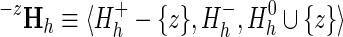and where Θ′ and α′ indicate the modified variables obtained upon replacement of H_h with .

To determine the contribution of subtree h′ to a specific supergroup (denoted as subLLR(h′, h)), we need to merely replace within Equation 4 z with h′ and with 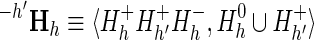, where . Computing the LLR_MAP contribution of a subhierarchy rooted at node h (denoted as H^h) is straightforward; it involves computing Equation 1 as if H^h were the entire hierarchy.

3.4. Evaluating sequence membership within each subgroup

We could estimate the probability of sequence membership within a subgroup by noting the frequency with which the sampler assigns each sequence to that subgroup during postconvergence sampling. However, this approach is very expensive computationally and, therefore, is not used here. Instead, the contribution to the subLLR(h) of sequence i is calculated by subtracting the corresponding subLLR when that sequence is removed from the foreground partition for contrast alignment h. That is,

where and and where Θ′ and α′ again indicate the resultant modified variables. Note that, because sequences are down weighted for redundancy, the influence of each member of a cluster of redundant sequences on the subLLR is correspondingly diminished. To offset this effect, the sequence's contribution to the subLLR is multiplied by the inverse of its fractional weight. This assumes that each member of its redundant set of closely related sequences makes, on average, the same contribution to the LLR_MAP. We will also compute the rank of each sequence i among the other sequences within the subgroup according to each subLLR(i, h). Finally, we similarly compute subLLR(i), defined as the contribution of sequence i to the total LLR. By examining a sequence's rank and its various contributions to the total LLR and subLLRs, we obtain a measure of confidence in that sequence's assigned sequence set. Note that for some sequences assigned to a subgroup h, the subLLR(i, h) may be negative. This does not necessarily indicate, however, that the assignment is wrong biologically; instead, it may indicate that the sequence is an atypical member of that subgroup. After all, in such cases, the sampler could have assigned the sequence either further up the hierarchy or to the root node background partition, which corresponds to sequences rejected as members of the domain class. Hence, a negative subLLR(i,h) may occur as a compromise over alternative assignments that are worse because of the various constraints imposed by the other features of the hierarchy; this situation is analogous to the principle of minimal frustration in protein folding (Bryngelson et al., 1995), where the energetic frustrations associated with conflicting interactions are minimized.

3.5. Assessing sequence and taxonomic diversity

To identify sequence determinants of protein function, it is important to distinguish conservation because of selective pressures from that merely due to recent common descent. It is currently unclear how to model this statistically; so, instead, we merely assess the sequence and taxonomic diversity of each node and subtree. Sequence diversity of a subtree h or a node z, denoted here by SqDv(h) and SqDv(z), respectively, is defined as the relative standard deviation (RSD) of the scores of each of the sequences against the consensus sequence for that subgroup. The RSD is the ratio of the standard deviation to the mean expressed as a percentage. The corresponding taxonomic diversity, denoted here by TxDv(h) and TxDv(z), is simply the number of phyla represented in the subgroup, where phyla are as defined by the NCBI taxonomy database (Federhen, 2012). Examining both SqDv and TxDv is helpful, as certain subgroups that consist entirely of taxonomically uncharacterized sequences may still be worthwhile modeling if their SqDv is high. Subgroups with low SqDv and high TxDv may similarly be worthwhile modeling.

3.6. Evaluating the contributions of conserved residues

One of the less obvious but important aspects of optimizing a protein domain hierarchy is to identify sequence determinants of protein function. Key catalytic residues at enzyme active sites are often conserved over long periods of evolutionary time. Of course, the same holds for many residues whose biological roles are still unknown. Hence, those subgroup-specific patterns that are subject to the strongest selective pressures are most likely to perform critical biological functions associated with that subgroup. As a measure of the selective pressure associated with subgroup-specific discriminating patterns, we compute the contribution of the jth pattern position in contrast alignment h as:

where

and where log Q(X,θ_h,j, α_h, A_h,j H_h, S) is defined analogously as for Equation 2.

4. Results

The approaches described in the previous section were implemented in C++ and applied to the 60 domains (from the NCBI CDD) that are described in Neuwald (2014). In this section, the evaluation and comparison of protein domain hierarchies is illustrated using two of the most challenging to model among these domains, namely, those related to the phosphoinositide 3-kinase (PI3Kc) catalytic domain (cd00142) and those related to phosphoribosyltransferase type II domains (PRTaseII) (cd00516). Because the PRTaseII domain is particularly challenging, it provides ample opportunity to apply the various approaches described in Section 3.

4.1. Comparing manually curated and automatically generated hierarchies

Figure 2 illustrates a comparison between two independently generated hierarchies using PI3Kc-like catalytic domains. One hierarchy was generated and optimized from a single root node (i.e., de novo) by the omcBPPS sampler, as described by Neuwald (2014), whereas the other was manually curated. For the curated hierarchy, the pattern and sequence assignments were optimized using the mcBPPS sampler (Neuwald, 2011) to obtain the associated LLR_MAP. The de novo hierarchy expands one of the leaf nodes in the curated hierarchy into a subtree and inserts three additional internal nodes (Fig. 2A), whereas the curated hierarchy expands two nodes within the de novo hierarchy into subtrees. Based on our metric, the de novo hierarchy achieved a slightly better score (56,085 nats) than did the curated hierarchy (56,514 nats). However, the de novo hierarchy is based on more stringent criteria regarding the number of phyla and the sequence diversity associated with the nodes (Fig. 2B,C). The lowest SqDv score for the sequence sets associated with the de novo hierarchy is 8.0 RSD, whereas for the curated hierarchy it is 5.3 RSD. Likewise, all of the nodes within the de novo hierarchy span at least three phyla, whereas the curated hierarchy has five nodes corresponding to a single phylum. The curated hierarchy models two leaf nodes of the de novo hierarchy as two subtrees, cd05165 and cd05166, with seven leaf nodes. In fact, the de novo hierarchy could not have retained these seven leaf nodes as they have fewer assigned sequences (35–55) than were permitted by the sampler (≥100 for this analysis). Thus, at least regarding these aspects of the curated hierarchy, the applied criteria were clearly less stringent. Applying the sampler de novo using these less stringent criteria resulted in a considerably larger hierarchy of 40 nodes with a score of 73,159 nats. Together, these analyses indicate that the optimized hierarchies constitute a significant improvement over the curated hierarchy in this case.

FIG. 2.

Comparison of various hierarchies for PI3Kc-like domains (cd00142). (A) Comparison between the Conserved Domain Database manually curated hierarchy (56,085 nats; 22 nodes) and a hierarchy generated de novo (56,514 nats; 20 nodes). Nodes are colored (as indicated) depending on whether they correspond (i.e., share ≥90% of their assigned sequences), roughly correspond (share >50%), or fail to correspond. The orange-highlighted line indicates that assignment of node cd05172 as a child of cd05164 lacks statistical support (i.e., the subLLR is negative). (B) Histogram of sequence diversity (SqDv) for the hierarchies shown in (A). (C) Scatter plot of SqDv versus the number of phyla for the curated and de novo hierarchies. RSD, relative standard deviation.

4.2. Comparing independently optimized hierarchies

Perhaps a more important type of comparison is between alternative, independently optimized hierarchies with a view to identifying and combining the most robust features and thereby obtaining further improvements. To aid such comparisons we can also evaluate the various subLLR contributions described in Section 3. In this and the following subsections, such analyses are performed on three independently generated and optimized hierarchies for PRTaseII-related domains, comparisons between which are shown in Figure 3. These hierarchies share a significant number of nodes and five major subtrees in common. Indeed, two of the subtrees, those rooted at nodes 29 and 40 in the figure, are essentially identical within all three hierarchies, indicating good support. However, the manner in which these five subtrees are arranged differs. The subLLR scores for each subhierarchy corresponding to these major subtrees (bottom of Fig. 3) indicate comparable support for each of these alternative arrangements. Although the LLR score for the hierarchy A in Figure 3 (178,463 nats) is about 5% less than the highest scoring hierarchy, the scores for the two remaining hierarchies (B and C) are nearly identical (186,731 nats vs. 186,359 nats). In the following subsections we investigate why these different subtree arrangements may have such similar levels of support.

FIG. 3.

Independently optimized hierarchies for PRTaseII-related domains (cd00516). (A) A hierarchy optimized starting from a heuristically generated hierarchy. (B) A hierarchy optimized starting from a single root node (i.e., de novo). This (highest scoring) hierarchy serves as the reference for the other two hierarchies. (C) A hierarchy optimized starting from a manually curated hierarchy. Nodes in each full hierarchy are colored as indicated in Figure 2, but with some of the nodes in (B) two-toned to indicate that each of those nodes differs in correspondence with a node in (A) (top color) versus a node in (C) (bottom color). These three hierarchies share five subtrees in common (although utilizing distinct arrangements thereof). Each of the root nodes of these subtrees is highlighted in the full hierarchies with glow that is similarly colored as is the corresponding node in the truncated hierarchy below. These subtrees are investigated further here. For the truncated hierarchies, the LLR contribution (in nats) to the subhierarchy [i.e., subLLR(H^h), where h corresponds to the associated node] and to the contrast alignment [i.e., subLLR(h)] are indicated by the numbers shown in black and red, respectively.

4.3. Examining contributions of individual nodes and patterns

Figure 4 examines the LLR contributions of nodes and patterns to the contrast alignment associated with the main root node of the highest scoring PRTaseII hierarchy (shown in Fig. 3B). The contribution of each node is displayed in a plot subLLR(z,h) above a corresponding heat map of the percentage of sequence matches to pattern residues for each node. Even though, for this contrast alignment, all of the nodes are assigned to the foreground partition, those nodes belonging to subtrees 29 and 40 (color coded in purple and orange, respectively, in the figures) lack matches to a significant number of pattern residues. As a result, removing the sequences corresponding to these nodes actually increases the overall LLR—as indicated by their negative values of subLLR(z,root) (see plot in Fig. 4)—presumably by improving the proportion of foreground sequence pattern matches. This does not imply, however, that these subtrees are unrelated to the other foreground sequences or that they are misclassified, for two reasons: first, they still retain a significant number of pattern matches to the consensus for the class; second, the sampler did not assign them to the background (unrelated sequence) partition. Notably, the patterns that subtree 29 sequences lack are largely distinct from those absent from subtree 40 sequences, and none of the three hierarchies in Figure 3 (nor others that we examined) grouped subtrees 29 and 40 together.

FIG. 4.

Heat map showing the percentage of sequences, among those assigned to each node (columns), that match each of the patterns (rows) associated with the root node contrast alignment for the de novo PRTaseII hierarchy. Plotted above the map are the values of subLLR(z,h) for the zth node and where h corresponds to the root; node identifiers are listed in the row directly below the map. Node identifiers are highlighted using the subtree color scheme given in Figure 3. Note that all of the nodes in two of the subtrees (highlighted in purple and orange) contribute negatively to the LLR. Nodes are ordered by decreasing percentages of overall matches to the patterns; note that this fails to correspond to decreasing values of subLLR(z,h) because the number of sequences (shown in the bottom row) influences this value, but not the percentage of matches. The contributions (in nats) of patterns, denoted by subLLR(j,h), are given in the far right column.

Further insight is provided by examining, in the same way, the foreground and background partitions associated with the major subtrees of PRTaseII hierarchy B. The heat map in Figure 5A reveals that, despite subtree 29 lacking certain canonical patterns, it also shares with subtree 2 conserved patterns that distinguish these from the remaining subtrees. Note too that each of the foreground nodes are well supported [see plot of subLLR(z,h) in this figure]. This explains why node 49 links these subtrees together in hierarchy B. This heat map also suggests why hierarchy A in Figure 3 links these subtrees to subtrees 3 and 40: Among the background nodes in the map, subtrees 3 and 40 share certain foreground patterns that subtree 48 lacks. The heat map corresponding to the subtree 3 contrast alignment in Figure 5B likewise reveals that certain patterns distinctive of subtree 3 also match sequences within subtrees 2 and 29 and, to a lesser extent, subtree 40. Conversely, the heat map in Figure 5C for the contrast alignment with subtree 2 in the foreground and subtree 29 in the background indicates that subtree 3 shares certain foreground patterns—as does subtree 48. The subtree 40 contrast alignment, however, fails to exhibit such pattern sharing (Fig. 5D). Finally, the heat map in Figure 5E, for which subtree 29 is in the foreground and subtree 2 in the background, indicates that subtree 48 conserves a few foreground patterns—though these appear to be due to chance as those sequences assigned to the unrelated sequence (i.e., random background) set match a similar percentage of foreground patterns. Patterns conserved in subtree 48 (Fig. 5F) also appear unique to that subtree.

FIG. 5.

Heat maps of contrast alignment sequence-to-pattern matches for major subtrees within the de novo (optimized) PRTaseII hierarchy in Figure 3B and, for three of these, subLLR(z,h) plots. Rows and columns in each heat map correspond to patterns and nodes, respectively, as in Figure 4. Using the same color scheme as in Figure 3, the blocks above each map indicate to which subtree the node in that column belongs. The blue and red horizontal bars directly below each map correspond, respectively, to the foreground and background partitions for each contrast alignment; the short black bar corresponds to the rejected sequence node; the remaining nodes are assigned to the nonparticipating partition. (A) The heat map and plot associated with the subtree rooted at node 49. (B) Subtree 3 heat map. The subLLR(z,h) is >1,571 nats for each foreground node z. Note that background nodes for subtrees 2, 29, and 40, but not 48, share some pattern matches with the foreground. (C) Subtree 2 heat map and plot. (D) Subtree 40 heat map. The subLLR(z,h) is >2,352 nats for all foreground nodes. (E) Subtree 29 heat map and plot. Note that the subLLR(z,h) for both nodes 35 and 46 is slightly negative (plotted in red). (F) Subtree 48 heat map. The subLLR(z,h) is >444 nats for all foreground nodes.

Hence, the manner in which conserved and divergent residues are distributed across these subtrees is somewhat inconsistent with a single hierarchy: The analysis in Figure 5C indicates that subtrees 2 and 48 share patterns that distinguish these from subtree 29, whereas the analysis in Figure 5A indicates that subtrees 2 and 29 share patterns that distinguish these from subtree 48. Similarly, Figure 5A indicates that subtrees 2 and 29 share certain patterns with subtrees 3 and 40, which may explain why hierarchies A and C in Figure 3 connect these four subtrees differently.

4.4. Comparing node and pattern contributions across hierarchies

The heat map and subLLR(z,h) plot in Figure 6A, which corresponds to the subtree rooted at node X of hierarchy A, further aid the evaluation of this alternative subtree arrangement. The foreground for this subtree corresponds to the (sub-)subtrees 29, 2, 3, and 40. This heat map delineates more clearly the patterns shared by these subtrees. However, the corresponding plot reveals that the nodes associated with subtrees 3 and 40 contribute negatively to the contrast alignment subLLR associated with subtree X. This appears because of these subtrees both lacking some of the subtree X patterns and matching more frequently other patterns that background nodes also tend to match. Hence, this helps account for the lower overall LLR score for hierarchy A and the notion that hierarchy B is a better model.

FIG. 6.

Heat maps of contrast alignment sequence-to-pattern matches and subLLR(z,h) plots for major subtrees within the lower scoring PRTaseII hierarchies A and C of Figure 3. In each map, the red vertical line divides positively contributing foreground nodes (green bars in the plot on the right) from those with negative contributions (red bars). See the legends to Figures 4 and 5 for further descriptions. (A) Heat map and plot for subtree h = X of hierarchy A. (B) Heat map and plot for subtree h = Y of hierarchy C. (C) Heat map and plot for subtree h = yy of hierarchy C.

A similar analysis of subtree Y within hierarchy C provides additional support for hierarchy B. Figure 6B shows the associated heat map and subLLR(z,h) plot. The foreground for this subtree includes the (sub-)subtrees 29, 2, and 3. Unlike the analysis of subtree 49 within hierarchy B (see Fig. 5A), for which the node subLLR contributions are all positive, the nodes associated with subtree 3 again contribute negatively to the subLLR for subtree Y. This appears because of subtree 3 both lacking some of the foreground patterns and matching other of these patterns that background nodes in subtree 40 (and, to a lesser extent, subtree 48) also match. This again supports hierarchy B as the better model.

Because the heat maps in Figure 5B and C suggest that subtree 3 may be more closely related to subtree 2 than to subtree 29, Figure 6C examines subtree yy in hierarchy C, which links subtrees 2 and 3. The heat map indicates that many of the foreground patterns shared by subtrees 2 and 3 are also conserved in subtrees 48 and 40. Furthermore the subLLR(z,h) plot again indicates that subtree 3 contributes negatively, as in Figure 6B. Together, these analyses suggest that hierarchy B is the best. However, the observed patterns of sequence conservation and divergence in this domain class appear to create ambiguities leading to alternative, nearly optimal trees. Moreover, as discussed below, a single tree-based hierarchy appears to inadequately model all such patterns.

4.5. Examining signature residues and evaluating alignment quality

The heat maps in Figures 4–6 are based on the discriminating patterns associated with specific levels of a hierarchy. These patterns also provide useful information regarding sequence determinants of protein function. This is illustrated in Figure 7. Figure 7A shows the hierarchical path from the root to node 14. A contrast alignment is associated with each node along such a path, each of which reveals those conserved residues that most distinguish the subtree associated with that node from closely related sequences associated with its parent and the parent's other descendant nodes. Figure 7C shows the contrast alignments for the first three nodes on this path to node 14. The height of the red bar above each highlighted aligned column j corresponds to the value of subLLR(j,h) for the pattern at that position. Figure 7B shows the structural locations of the residues matching the highest scoring patterns in these contrast alignments; notably, they all occur within the substrate-binding pocket. This is typical of conserved residues associated with nodes higher up in a hierarchy for substrate-binding proteins; thus, such subLLR scores can provide clues to biological function, which is unsurprising, of course, given that strong selective pressures are presumably maintaining these patterns. The highest scoring patterns lower down in the hierarchy presumably are also involved in biological functions subject to strong selective pressure, though it is typically unclear what these functions might be. Identifying such residues, however, is a helpful first step toward characterizing underlying determinants of biochemical functions and mechanisms.

FIG. 7.

A hierarchy of contrast alignments revealing pattern residues. (A) The path from the root to node 14 in PRTaseII hierarchy B. (B) Pattern residue structural locations within Mycobacterium tuberculosis quinolinate phosphoribosyltransferase in complex with phthalate and a substrate analog, PRPCP (1QPR) (Sharma et al., 1998). The highest scoring pattern residues in (C) are shown. (C) Contrast alignments associated with the root and with nodes 48 and 47. Representative aligned sequences (which were assigned to node 14) are highlighted to reveal pattern residues; the red dots indicate the residues shown in (B). Foreground and background residues at each position are shown below each alignment, and directly below these, corresponding frequencies are given in integer tenths (a “7,” for example, indicates 70–80% conservation). The bar height above each highlighted column j corresponds to subLLR(j,h).

Such contrast alignments are associated, of course, with every node in a hierarchy. Collectively, these provide extensive information, not only regarding biologically relevant protein properties, but also regarding the quality of the input alignment used to construct the hierarchy. Thus, these contrast alignments can be used to evaluate and improve the alignment, ideally in conjunction with crystal structure data. Misaligned regions typically show up as sequence regions that lack matches to pattern residues at various levels of the hierarchy. Once an input alignment that is misaligned is corrected in this way, an omcBPPS analysis can be repeated to improve the hierarchy, and this process can be repeated iteratively until a high-quality input alignment and corresponding hierarchy is obtained.

4.6. Analysis of sequence contributions

Examining sequence subLLR contributions can identify those sequences most typical of a subgroup and thereby facilitate biological interpretation in the light of crystal structure data and of the biological literature. It can also determine whether most of the sequences assigned to a specific subgroup share the features of that subgroup in roughly equal measure or whether there is considerable variability between sequences. Sequences may diverge from signature patterns because of true functional divergence, in which case there may be insufficient numbers of such sequences to form a separate subgroup causing them, instead, to be assigned to the most closely related subgroup. Alternatively, such divergence may be caused by random mutations within pseudogenes or to sequencing errors.

Figure 8 illustrates how the sequence subLLR metric can be used to identify and characterize sequence divergence. It focuses on node 73 of PRTaseII hierarchy B, the path to which from the root node is shown in Figure 8A. Figure 8B shows a histogram of the LLR contributions of each of the sequences assigned to this leaf node; this reveals a bimodal distribution for which the contributions of 8 out of the 42 assigned sequences are negative (termed Set73N) and positive for the rest (termed Set73P). The heat map shown in Figure 8C, which partitions this sequence set into negative and positive contributors, reveals that the sequences in Set73N lack roughly half of the signature patterns characteristic of node 73. This divergence does not appear to be due to sequencing errors or to pseudogenes because the subLLR scores for the six other contrast alignments, in which these sequences are assigned to the foreground partition, are all positive (Fig. 8D). Presumably, mutations in genes lacking selective pressure or sequencing errors would occur more or less uniformly across all of these categories, which is not the case here. Thus, it appears that the sequences in Set73N constitute a sub-subgroup that is currently too small to form a distinct node.

FIG. 8.

Contributions of individual sequences. (A) Path from the root to node 73 in PRTaseII hierarchy B. (B) Histogram showing the LLR contributions of the sequences assigned to node 73. This reveals a bimodal distribution, with 8 negative and 34 positive subLLR(i, h = 73) contributors. These sequence sets are denoted as Set73N and Set73P, respectively. (C) Heat map of foreground (Set73P, Set73N) and background (Set15, Set27) sequence sets associated with the node 73 contrast alignment. (D) Bar graph showing the subLLR(i,h) contributions and percentile rank of the poorest scoring sequence in (B), namely, nicotinate phosphoribosyltransferase from Bacillus methanolicus PB1; below are shown the corresponding nodes, which occur along the path shown in (A). (E) Histogram showing the LLR contributions of the sequences assigned to subtree 15. The red arrow indicates the score for the sequence in (D).

Again, it should be noted that a negative subLLR score does not necessarily mean that the sequence does not belong in the assigned subgroup. The sampler could have moved it further up the hierarchy or assigned it to the “reject” category instead of to that subgroup. Thus, the sampler (with simulated annealing) presumably found a nearly optimal assignment for that sequence versus the various other options. (Note that the subLLR is computed by eliminating the sequence from the alignment hierarchy, which is not an option during sampling. Thus, if eliminating a sequence enhances conservation of pattern residues in the remaining sequence set, then the subLLR contribution of that sequence will be negative.) Thus, Set73N appears to correspond to atypical members of the node 73 subgoup. Nevertheless, our confidence in subgroup assignments will, of course, be lower for sequences with negative subLLR scores.

5. Discussion and Conclusion

Proteins appear to evolve in fits and starts inasmuch as related sequences tend to cluster into subgroups each of which share conserved patterns distinguishing them from other, related sequences. This has motivated the construction of protein domain hierarchies, each of which arranges related subgroups into a tree for which descendent nodes generally conserve patterns present in their ancestral nodes. Until recently, constructing such hierarchies has been performed manually, even though doing so optimally is a very challenging algorithmic problem. Indeed, for the most challenging domains, even independent runs of our automated sampler tend to converge on somewhat different hierarchies, thereby underscoring the difficulty of this problem.

For a hierarchy characterized by a complex arrangement of nodes, it is possible that combining various aspects of differing hierarchies could lead to a further improved, recombinant hierarchy. This requires the ability to compare various hierarchies and to measure the contribution to the total LLR of each subfeature to be recombined. Such comparisons and measures can also provide a deeper understanding of the nature of functional divergence within a protein class and thus may lead to new evolutionary insights and/or to the identification of subgroup-specific sequence determinants of protein function. Such measures can also provide rapid estimates of levels of confidence regarding assigned functional classifications, which is relevant to genome annotation. Likewise, an analysis of taxonomic and sequence diversity can ensure that curation criteria are applied in a consistent manner. For these reasons the approaches described here for evaluating, comparing, and interpreting domain hierarchies should be helpful.

These approaches can also reveal ways to improve automated methods for constructing and utilizing hierarchies. For example, the subLLRs associated with the major subtrees of the two nearly optimal PRTaseII hierarchies (B and C in Fig. 3) suggest that recombining aspects of both might lead to an improved hierarchy. This suggests that development of a genetic-algorithm version of the omcBPPS sampler would be useful. These approaches can also provide algorithmic insights leading to more efficient sampling operations, which could provide accurate estimates both of a hierarchy's relative entropy and of predictive probabilities for sequence subgroup assignments and other hierarchical features.

The PRTaseII analysis (and similar analyses not described here) reveals that patterns of conserved and divergent residues may not follow a single tree-based hierarchy. As a result, certain conserved patterns may be assigned inappropriately or not at all. One way to accommodate such misfit patterns is to redefine the underlying statistical model using the mathematically more general notion of a hierarchy as a directed acyclic graph (DAG). This would avoid presuppositions regarding what sort of evolutionarily events are possible and would thereby accommodate (and, in fact, reveal) confounding events, such as paralogous recombination or loss of certain ancestral properties. A DAG-based sampler would accommodate such events by defining additional internal nodes linked arbitrarily to subtrees that harbor confounding patterns further down the hierarchy. This could reveal biologically important residues conserved across evolutionarily distant subgroups in an inconsistent manner. With these benefits in mind, the approaches described here are being incorporated into the NCBI CDD curation pipeline.

Acknowledgment

This work was supported by the School of Medicine at the University of Maryland, Baltimore and by NIH contract HHSN 2630000999571.

Author Disclosure Statement

No competing financial interests exist.

References

- Bryngelson J.D., Onuchic J.N., Socci N.D., and Wolynes P.G.1995. Funnels, pathways, and the energy landscape of protein folding: a synthesis. Proteins 21, 167–195 [DOI] [PubMed] [Google Scholar]
- Cover T.M., and Thomas J.A.1991. Elements of Information Theory. John Wiley & Sons, Inc., New York [Google Scholar]
- Federhen S.2012. The NCBI taxonomy database. Nucleic Acids Res. 40, D136–D143 [DOI] [PMC free article] [PubMed] [Google Scholar]
- Felsenstein J.2004. Inferring Phylogenies. Sinauer Associates, Sunderland, MA [Google Scholar]
- Liu J.S.2008. Monte Carlo Strategies in Scientific Computing. Springer-Verlag, New York [Google Scholar]
- Marchler-Bauer A., Anderson J.B., DeWeese-Scott C., et al. 2003. CDD: a curated Entrez database of conserved domain alignments. Nucleic Acids Res. 31, 383–387 [DOI] [PMC free article] [PubMed] [Google Scholar]
- Marchler-Bauer A., Lu S., Anderson J.B., et al. 2011. CDD: a Conserved Domain Database for the functional annotation of proteins. Nucleic Acids Res. 39, D225–D229 [DOI] [PMC free article] [PubMed] [Google Scholar]
- Neuwald A.F.2011. Surveying the manifold divergence of an entire protein class for statistical clues to underlying biochemical mechanisms. Stat. Appl. Genet. Mol. Biol. 10, 36. [DOI] [PMC free article] [PubMed] [Google Scholar]
- Neuwald A.F.2014. A Bayesian sampler for optimization of protein domain hierarchies. J. Comput. Biol. 21, in press. [DOI] [PMC free article] [PubMed] [Google Scholar]
- Neuwald A.F., and Green P.1994. Detecting patterns in protein sequences. J. Mol. Biol. 239, 698–712 [DOI] [PubMed] [Google Scholar]
- Neuwald A.F., Lanczycki C.J., and Marchler-Bauer A.2012. Automated hierarchical classification of protein domain subfamilies based on functionally-divergent residue signatures. BMC Bioinformatics 13, 144. [DOI] [PMC free article] [PubMed] [Google Scholar]
- Sharma V., Grubmeyer C., and Sacchettini J.C.1998. Crystal structure of quinolinic acid phosphoribosyltransferase from Mycobacterium tuberculosis: a potential TB drug target. Structure 6, 1587–1599 [DOI] [PubMed] [Google Scholar]