Abstract
A wealth of methods has been developed to identify natural divisions of brain networks into groups or modules, with one of the most prominent being modularity. Compared with the popularity of methods to detect community structure, only a few methods exist to statistically control for spurious modules, relying almost exclusively on resampling techniques. It is well known that even random networks can exhibit high modularity because of incidental concentration of edges, even though they have no underlying organizational structure. Consequently, interpretation of community structure is confounded by the lack of principled and computationally tractable approaches to statistically control for spurious modules. In this paper we show that the modularity of random networks follows a transformed version of the Tracy-Widom distribution, providing for the first time a link between module detection and random matrix theory. We compute parametric formulas for the distribution of modularity for random networks as a function of network size and edge variance, and show that we can efficiently control for false positives in brain and other real-world networks.
Keywords: functional connectivity, community structure, graph partitioning methods, modularity, random graphs
1. Introduction
The complexity in the macroscopic behavior of brain networks has been highlighted and quantified in a number of neuroscience studies in recent years (Bullmore and Sporns (2009); Rubinov and Sporns (2010)). A multitude of topological features has been reported in the literature, including modular structures (Bullmore and Bassett (2011); Chang et al. (2012)), hierarchical patterns (Salvador et al. (2005); Meunier et al. (2009)), distribution of hubs (Sporns et al. (2007); Tomasi and Volkow (2011); Dimitriadis et al. (2010)), and core extraction (Hagmann et al. (2008a)). It has also been shown that brain networks follow a small-world property both from a functional (Bassett and Bullmore (2006); Van den Heuvel et al. (2008)) and a structural perspective (Vaessen et al. (2010); Wang et al. (2012)). Recent findings have revealed alterations of brain network topology with aging (Chen et al. (2011)), brain development (Fan et al. (2011)), and pathologies of schizophrenia, autism, and epilepsy (Alexander-Bloch et al. (2010); Rudie et al. (2013); Chavez et al. (2010)), underscoring the importance of networks as biomarkers of the normal and diseased brain.
Fundamental to identification of the architecture and organization of brain networks is the detection of modules, also called communities or clusters. In the context of graph theory, modules are groups of interconnected nodes, typically regions of parcelated cerebral cortex, that share common properties or have similar function within the network. Identification of modules can facilitate the prediction and discovery of previously unknown connections and components, and show how the network constitutes a collective and integrative system. Individual nodes can be classified according to their structural position in the modules; nodes with central position are essential for the stability and robustness of their corresponding modules, and nodes lying at the boundaries contribute to interactions across communities. Studies of network topology can reveal important properties of brain organization, for exampling revealing potential vulnerabilities, or in the case of hierarchical networks, possibly encoding clues to the evolution of the brain (Meunier et al. (2010)).
Underscoring the central role of module detection, numerous methods have been proposed to identify community structure in brain networks. Perhaps the most popular is modularity (Newman (2006)), which compares the network against a null model and favors within-module connections when edges are stronger than their expected values. Divisions that increase modularity are preferred because they lead to modules with high community structure. We recently proposed a new method to compute network null models based on conditional expected probabilities and provided exact analytical solutions for specific parametric distributions (Chang et al. (2012)). Our models enhance module detection, provide a principled approach to deal with networks with negative connections, and accurately represent the topology of networks without necessitating self-loops.
Despite the popularity of modularity methods, the identification of stopping criteria for graph division and the evaluation of the statistical significance of modules remain largely unaddressed. Given that random networks can demonstrate spurious modules due to incidental concentration of edges, even though they have no underlying organizational structure, controlling for false positives in community detection is of paramount importance. This is even more evident in large networks where the number of possible divisions increases rapidly with the network size (Guimerá et al. (2004); Karrer et al. (2008)). Therefore, confirming the statistical significance of any identified modules is essential before discussing other findings related to those structures.
Existing methods that control for spurious modular structures fall into three categories. The first category relies on creating comparable random networks in order to compute an empirical null distribution of modularity and establish a threshold that controls error rate at a nominal level, typically 5%. For example, Alexander-Bloch et al. (2010) estimated the distribution of modularity using two types of random networks, the Erdös-Rényi random graphs (Erdős and Rényi (1960)) or randomly rewired networks (Maslov and Sneppen (2002)). Meunier et al. (2009) created random networks by randomizing either the elements of the adjacency matrix, or the time points of the time series whose pairwise correlation defined the edges of a graph. He et al. (2009) generated a set of node- and degree-matched random graphs for comparison. Reichardt and Bornholdt (2006) computed the z-values of modularity after estimating its empirical distribution through multiple random network realizations. Mirshahvalad et al. (2013) studied how different resampling schemes influence significance analysis.
The second category of methods also relies on resampled networks. Here the aim is to measure the robustness of modular structures on network perturbations. For instance, Karrer et al. (2008) proposed a method to perturb network connections and measure the resulting change in community structure using mutual information. Hu et al. (2010) offered a generalization to this approach by incorporating together the number of clusters, content of the clusters, and random perturbation parameters. Mirshahvalad et al. (2012) studied the robustness of large sparse networks by randomly adding extra links based on local information. Lancichinetti et al. (2010) evaluated the importance of single communities using combinatorics and a modified null model. Seifi et al. (2012) measured the significance of modules based on the stability of structures from either randomly perturbed networks or different initialization of non-deterministic community detection techniques.
Since all the above methods depend on edge rewiring and random network realizations, they are network-specific and do not generalize. The computational cost of generating multiple realizations of random networks can be significant, and even prohibitive for very large networks in the order of thousands of nodes. The third category of methods offers analytical closed-form solutions for the distribution of modularity in random networks. To the best of our knowledge, due to the complex form of the modularity function, there exists only one closed form solution for a specific case. Reichardt and Bornholdt (2007) used the Potts spin-glass model to get a theoretical prediction for modularity value in binary random graphs, either Erdös-Rényi type or scale-free random networks. However, their formula is restricted to binary sparse networks, which prevents its use with most real-world networks.
Given the lack of a principled analytical approach or computationally efficient algorithms to control for false positives in network module detection, much of the literature overlooks statistical inference in networks. To address this problem we provide a new analytical approach for statistical inference in module detection. Modularity belongs to the wide class of spectral clustering algorithms (Von Luxburg (2007)), which use the extreme eigenvalues and corresponding eigenvectors of a spectral decomposition to partition data into groups with similar properties. To evaluate the statistical significance of spectral clustering results, we need to compare the spectral decomposition of a given network against those from random networks. Since networks are represented by their adjacency matrix, a connection between random networks and random matrix theory is natural. The eigenvalue distribution of a specific type of matrices, Gaussian random ensembles, has been thoroughly studied in random matrix theory (Tracy and Widom (2000); Tao (2012)). In this paper, we provide for the first time a link between module detection and random matrix theory by showing that the Tracy-Widom mapping of the largest eigenvalue of Gaussian random ensembles can be modified to predict the distribution of the largest eigenvalue of matrices used for modularity-based spectral clustering. Using this finding, we derive an accurate parametric form of the distribution of modularity in random networks and compute formulas that control the type I error rate at a 5% level on modularity-based partitions of weighted graphs. Our modeling is valid for a wide range of network sizes and the utility of the method is all the more important for larger networks, given that resampling methods can be computationally infeasible in such networks. We demonstrate our method in brain and other real-world networks.
2. Methods
In this section, we first describe the modularity partitioning problem and its solution using spectral decomposition. We then motivate the use of the maximum eigenvalue of a difference matrix (adjacency matrix minus the null model) as a surrogate of modularity. Using a transformed Tracy-Widom distribution, we derive empirical parametric formulas that accurately predict the distribution of the maximum eigenvalue. We estimate our model parameters through Monte Carlo simulations of weighted Gaussian random networks.
2.1. Overview to Modularity
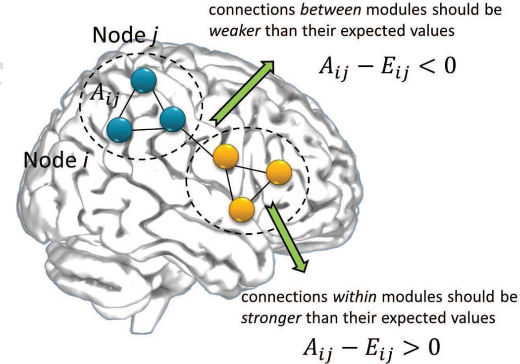
Large-scale brain networks are typically constructed by assigning nodes to represent regions of parcelated cerebral cortex and edges to represent the pair-wise interactions or connection across these regions. These connections could be based on structural data, for example white matter fiber-tracts derived from diffusion data, or functional coupling measured between time series of brain activation. Assume a brain network of N nodes with weighted undirected connections and an underlying modular structure, as exemplified in Figure 1. The network is represented with an adjacency matrix A with elements Aij indicating the connection strength across nodes i and j. The degree vector k has elements , equal to the sum of all edge strengths associated with node i. The total sum of edge weights of the network is denoted as .
Figure 1.
Brain networks and modularity.
Modularity was originally introduced as a measure of the quality of a particular division of a network (Newman and Girvan (2004)), but later became a key graph clustering algorithm, after recognizing its direct maximization using spectral graph partitioning (Newman (2006)). According to modularity, the community structure of the network is compared against a null network, i.e. a randomized network with the same number of nodes and node degrees but otherwise no underlying structure. If a natural division of a network exists, we should expect within-module connections Aij to be stronger than their expected values Eij, and the opposite should hold true for between-module connections (Figure 1). Modularity forms a cost function by summing all the within-module connections minus their expected values and divisions that increase modularity are preferred because they lead to modules with high community structure.
Fundamental to the definition of modularity is the computation of a proper null network. The conventional definition of modularity uses the null model proposed in (Newman (2006)):
| (1) |
However, in (Chang et al. (2012)) we recently proposed an alternative expected null model conditioned on the degree vector k:
| (2) |
Simulation results demonstrate that using our null model enhances module detection by properly dividing networks in a range of cases when the conventional approach fails to detect any modules. In part, this is because the conventional null model implicitly assumes self-loops (connections from nodes to themselves, Eij ≠ 0) which are often topologically invalid and meaningless for real-life networks, such as social, protein networks and the majority of brain networks. Furthermore, our null models provide a principled approach to deal with networks with negative connections across nodes. Before introducing our model, we were aware of only heuristic solutions that overcame the problem of negative edges by requiring a selection of weighted coefficients that subjectively influence clustering results (Gómez et al. (2009)).
Define B as the difference matrix between the original and the null network, with elements Bij = Aij − Eij. Modularity Q is defined as:
| (3) |
where Ci indicates the module membership of node i, and δ(Ci, Cj) = 1 only when nodes i and j are clustered withing the same module.
Modularity Q is maximized when the partitions align exactly with the underlying network structure. In the case of sequential partitioning, each bi-partition of the graph can be described by an indicator vector s having values 1 and −1 for the two subnetworks respectively, and computed as:
| (4) |
Spectral graph theory solves for ŝ in the continuous domain and achieves maximization by selecting the eigenvector corresponding to the largest eigenvalue λ1 of B. The elements of s are then discretized to −1, 1 by setting a zero threshold. Because of this discretization, further fine tuning is necessary to locally maximize Q, which can be done using, for example, the Kernighan-Lin algorithm. Given that the final maximum value of modularity Q is close to λ1, we can use the latter as a surrogate for modularity.
2.2. Distribution of modularity and error rate
Random networks can exhibit high modularity because of chance coincidence of edge positions rather than a true organizational structure. In fact, we can show that modularity algorithms are certain to produce spurious clusters in random graphs with Gaussian distribution of edges having zero mean and unit variance (Also see Section3). Therefore, using maximization of modularity as a sole criterion is bound to lead to false community detection. As discussed earlier, perhaps the most popular methods to control for false positives consider a graph partition as statistically significant if modularity Q is substantially higher than the one achieved by partitioning random graphs. They therefore compute an empirical null distribution of modularity and establish a threshold that controls error rate at a nominal level, typically 5%.
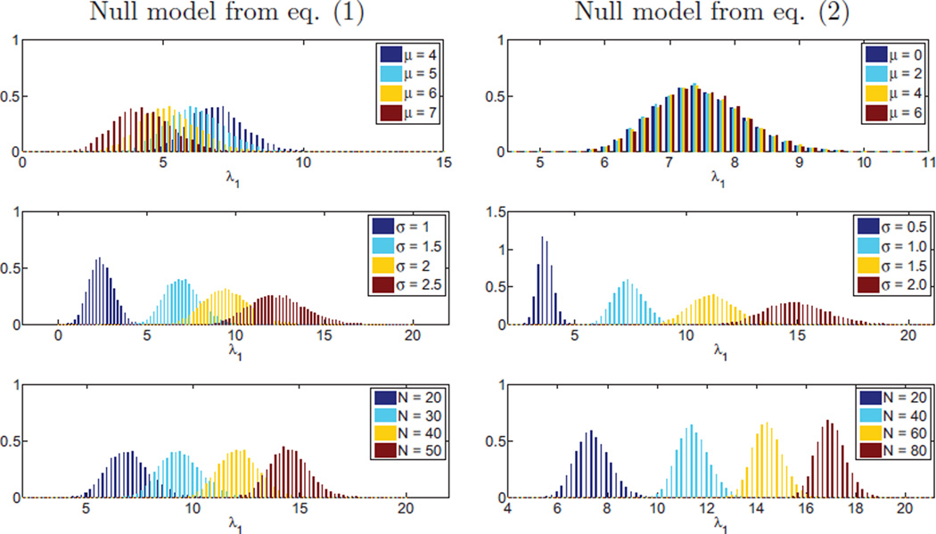
We follow a similar approach in this paper, namely we test whether the maximum eigenvalue of matrix B of the original network is appreciably higher (say 5% significance level) than the distribution of eigenvalues of matrices BRandom of random graphs. Unlike other approaches, though, we assume a specific parametric (Gaussian) distribution of the network edges, which allows us to derive formulas for the null distribution of modularity. The distribution we seek to model is shown in Figure 2 for random networks with Gaussian distribution of edges, as a function of edge mean μ, variance σ2, and networks size N. The maximum eigenvalue of matrix B is used as a surrogate of modularity. We observe that, unlike the conventional model (equation (1)), our null model (equation (2)) produces a distribution of modularity that is independent of μ. We limited simulations for the conventional model to high values of μ because equation (1) cannot accept negative edges.
Figure 2.
Distribution of the largest eigenvalue of BRandom over several network parameters. Left column: using the conventional definition of modularity, the distribution depends on the network size and the edge mean and standard deviation; right column: using our null model for the definition of modularity, the distribution becomes invariant to the edge mean.
2.3. Modeling using the Tracy-Widom Distribution
Random networks can be represented by their adjacency matrices and therefore be modeled as random matrices. In random matrix theory, the distribution of the largest eigenvalue of a wide class of random matrices, Gaussian random ensembles, has been related through a linear transform to the Tracy-Widom distribution (Tracy and Widom (2000); Johansson (2000); Johnstone (2001); Edelman and Rao (2005); Tao (2012)). Appendix Appendix A provides a brief introduction to this theory, and particularly the Gaussian orthogonal ensembles, which are real symmetric matrices with elements following an independent identical Gaussian distribution.
There are a couple of issues that prevent us from directly applying this theory to modularity-based spectral partitioning. First, even though Gaussian random networks can be represented as Gaussian orthogonal ensembles, modularity-based partitioning performs spectral decomposition on matrix B, the difference between the original and the null network. This introduces dependencies across the elements of the matrix B, thus violating the independence assumption in the Tracy-Widom mapping. Second, the Tracy-Widom distribution is an asymptotic property of the matrix size (or equivalently the network size) becoming more accurate as the number of nodes tend to infinity (Tracy and Widom (2000)). Brain networks have finite numbers of nodes, mostly ranging from tens to thousands of nodes, therefore we need parametric formulas that are reasonably accurate even for small networks.
In the case of Gaussian orthogonal ensembles, the scaling formula that predicts the distribution of the maximum eigenvalue is (see Appendix Appendix A for details):
| (5) |
where T is a random variable equal to the largest eigenvalue of Gaussian orthogonal ensembles, and S follows the Tracy-Widom distribution. Motivated by the above mapping, we seek a similar expression for the modularity case. If T is a random variable equal to the maximum eigenvalue of B (the difference between random Gaussian networks and their null models) we aim to find a mapping:
| (6) |
where w1(N, σ) and w2(N, σ) are power functions of the form:
| (7) |
| (8) |
Given the complex form of matrix B, analytical derivation of α1,2, β1,2, and γ1,2 parameters is a daunting task. Therefore, in the following section we resort to Monte Carlo simulations to estimate these parameters.
Compared to the Gaussian orthogonal ensembles mapping, we introduce the additional constants γ1,2 to achieve a better numerical fit. Also, in the following we pursue this mapping only for the modularity definition using our null model in equation (2); the conventional null model in equation (1) produces eigenvalue distributions that depend on the mean value μ of edge weights (Figure 2) thus requiring a more complex mapping that is not within the scope of this paper. However, as argued in the Discussion Section, such mapping is possible for the conventional definition of modularity.
2.4. Estimation of modeling parameters
We estimate the parameters α1,2, β1,2, and γ1,2 with Monte Carlo simulations and numerical procedures as follows. Consider the mapping in equation (6) where S follows the Tracy-Widom distribution in equation (A.6), i.e. fS(s) = f1(s) = dF1(s)/ds. Using a Monte Carlo approach, we simulate multiple realizations of Gaussian random graphs ARandom for a given value of N and σ. For each graph, we compute BRandom using our null model in equation (2) and then estimate the empirical distribution of the largest eigenvalue, termed fT(t). The functional transformation in equation (6) indicates that ; we dropped the dependency on N and σ to ease notation. We use the total Kullback-Leibler divergence to measure the distance between the two distributions:
| (9) |
which we then minimize over w1 and w2:
| (10) |
Every minimization of the above equation produces a value for w1(N, σ) and w2(N, σ) for a specific pair (N, σ). By repeating the above procedure multiple times, we sample the two functions across the (N, σ) plane.
Direct minimization of equation (10) using gradient decent often leads to local minima rather that the global minimum. To overcome this problem, we used an informed initialization of the of the gradient decent algorithm, by taking advantage of the direct mapping between the cumulative density functions F1(s) and FT(t). For a number of values xi ∈ [0, 1] we derived the corresponding si and ti such that {si|F1(si) = xi} and {ti|FT(ti) = xi}. We then estimated the initialization values with a least-squares minimization:
| (11) |
The values were then used to initialize the gradient decent algorithm in equation (10).
Minimization of equation (10) produces extremely low KL divergence values, and therefore the fT(t) distribution can be approximated very accurately by the mapping in equation (6). Figure 3 shows that the KL divergence becomes smaller as N increases, which agrees with the asymptotic behavior of the Tracy-Widom distribution in random matrix theory.
Figure 3.
Left: Kullback-Leibler divergence between f1 and transformed fT distributions for different values of N. The plot is averaged across a range of edge variance values. Right: Plot of f1 and transformed fT distributions for N = 100, indicating that they are nearly identical.
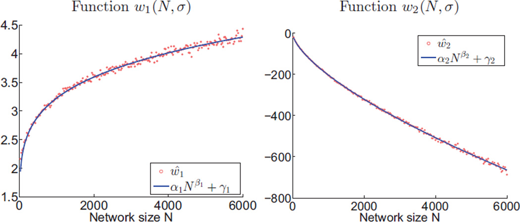
After sufficiently sampling the w1(N, σ) and w2(N, σ) functions in the (N, σ) plane, we performed a least square fitting of these samples to the power functions in equations (7) and (8) in order to estimate the model parameters. Since the Tracy-Widom distribution converges asymptotically, we performed two separate fits for small and large values of N to improve model accuracy. The first fit used 106 realizations of random networks for each of N values from 25 to 600 with step 25; the second fit used 4000 realizations of random networks for each of N values from 100 to 6000 with step 25. Table 1 shows the parameters estimates and their 95% confidence interval. Figure 4 illustrates that the power functions achieve a very accurate fit. For small networks, we explicitly set γ1 to zero because it does not improve the fitting accuracy.
Table 1.
Estimated parameters in equations (7) and (8) for small networks (left) and large networks (right). Also shown
| Network size N < 600 | Network size N ≥ 600 | ||
|---|---|---|---|
| parameter | estimated values | parameter | estimated values |
| α1 | 0.5795 ± 0.0153 | α1 | 0.6053 ± 0.0085 |
| β1 | 0.211 ± 0.0026 | β1 | 0.2019 ± 0.0011 |
| γ1 | 0.6869 ± 0.0228 | γ1 | 0.7824 ± 0.0161 |
| α2 | −2.071 ± 0.001 | α2 | −1.948 ± 0.199 |
| β2 | 0.6615 ± 0.0001 | β2 | 0.6695 ± 0.0111 |
| γ2 | 0 | γ2 | −4.96 ± 5.3086 |
Figure 4.
Illustration of fit between the estimated functions ŵ1 and ŵ2 (equation (10); shown as scatter plot) and the power functions (equations (7) and (8); shown as solid lines).
2.5. Significance Test
For every bi-partition of a graph, we can determine the significance of the cut by comparing the largest eigenvalue of B against the distribution of eigenvalues of BRandom. Therefore, rather than accepting a partition if it increases modularity Q, as is done by conventional modularity algorithms (Chang et al. (2012)), we test whether the increase is statistically significant above a 5% threshold. The procedure is given in the following steps:
For a network A, estimate edge variance σ2.
Apply spectral graph bi-partitioning and compute the largest eigenvalue λ1 of matrix B. (Chang et al. (2012)).
Estimate the value of functions w1(N, σ) and w2(N, σ) using the appropriate coefficients from Table 1, depending on network size N.
Compute w1(N, σ) λ1 + w2(N, σ) (i.e. linearly transform λ1 according to equation (6)), and compare this value against the Tracy-Widom distribution from equation (A.6). Accept the partition if the above value lies above the 5% threshold in the right tail of the distribution.
Repeat steps 2–5 until no subsequent bi-partitions are significant.
The above procedure constitutes a hierarchical order of statistical tests, each exploring the significance of a bi-partition only if the higher level bi-partition is deemed significant. The procedure controls family-wise error rate (FWER) at exactly α = 5% level, since the first bi-partition is tested at this level. However, this achieves only weak control of FWER, unless subsequent bi-partitions are controlled for multiple comparisons. For example, the threshold level can be adjusted with a Bonferroni approach (Hochberg and Tamhane (1987); Nichols and Hayasaka (2003)) depending on the number of bi-partitions tested simultaneously. A different approach is to use a hierarchical control of false discovery rate (Yekutieli et al. (2006); Singh and Phillips (2010)).
Open source code implementing the modularity-based partitions and statistical testing is available by contacting the first author, or visiting the address: http://mcgovern.mit.edu/technology/meg-lab/software.
3. Results
3.1. False Positives in Random Graphs
Maximization of modularity was originally proposed as a formal stopping criterion for graph division. Since the number of communities is typically unknown in advance, one could perform sequential bi-partitions that increase modularity until the entire network has been decomposed into indivisible subgraphs (Newman (2006)). In terms of spectral graph theory, a subgraph becomes indivisible if its corresponding difference matrix B has maximum eigenvalue equal to 0, in which case modularity no longer increases because there is no positive eigenvalue. Note that since B * 1 = 0 always holds (Chang et al. (2012)), 0 is always an eigenvalue of B with the unit vector 1 indicating a trivial partition where all nodes are grouped into one cluster leaving the other cluster empty.
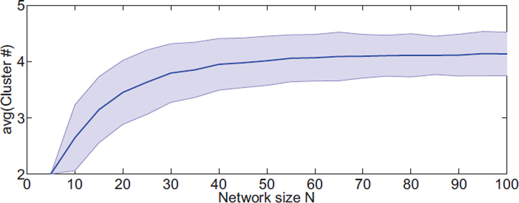
However, random networks often produce partitions that increase modularity. For example, in Figure 2 we illustrate that Gaussian random networks have difference matrix BRandom with almost always positive eigenvalues. Therefore, if we use maximization of modularity as a sole criterion for graph division, a single bi-partition leading to at least 2 clusters is practically guaranteed. Subsequent bi-partitions can further maximize modularity, leading to more spurious clusters. Figure 5 shows the number of spurious clusters obtained by bi-partitioning Gaussian random networks with edges having mean μ = 4 and unit variance. This highlights the need for statistical control of false positives.
Figure 5.
Average number of spuriously detected modules in random networks (false positives). Modules are identified by sequential bi-partitions of the networks while modularity, defined with the null model in equation (2), increases (objective function). Even though the simulated networks are completely random, we are certain to identify two or more modules, always leading to false detection of structure. Shaded region indicates ± one standard deviation.
3.2. Specificity of the Significance Tests
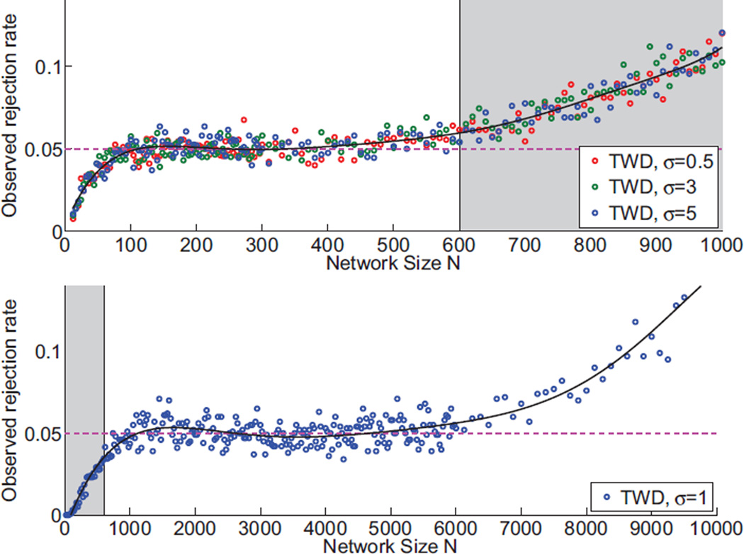
To test our parametric formulas for specificity, we generated networks with a range of sizes N and edge standard deviations σ, as indicated in Figure 6. We applied the 5% threshold procedure as summarized in section 2.5 and computed the observed null hypothesis rejection rate for this data set. Overall, our Tracy-Widom significance test achieves a rejection rate close to the nominal 5%. The test is based on two sets of formulas that apply either for large (N ≥ 600) or small (N < 600) networks. The performance of each formula deviates rapidly for values outside the allowed range, indicating the need for two rather than one set of parameters in Table 1. Also, the test becomes liberal for networks with N > 6000. We believe a more refined estimation of the parameters in Table 1 can extend the utility of our parametric formulas to considerably larger networks (see Discussion section for more details).
Figure 6.
Specificity of our statistical significance testing method based on the Tracy-Widom distribution (equation (6)). Plots show the observed null hypothesis rejection rate, when the nominal rate is α=5%. Solid lines indicate a polynomial fit across the measured scattered points. We suggest applying different sets of parameters with the boundary N = 600. Top panel shows the specificity for small networks and lower panel the specificity for large networks. Gray background indicates the specificity when our formulas are applied outside the suggested range. Notice, specificity does not depend on edge standard deviation.
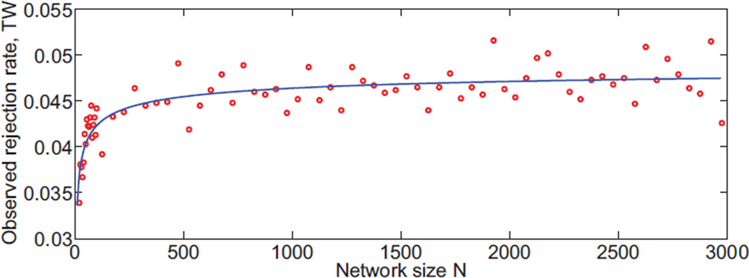
In part, our method is somewhat inaccurate for small N because it relies on the Tracy-Widom distribution (Equation (A.6)), which is an asymptotic description of the distribution of maximum eigenvalues of Gaussian orthogonal ensembles. To evaluate this asymptotic behavior, we performed a Monte Carlo simulation of Gaussian orthogonal ensembles and compared the nominal with the numerical estimates of their 5% right tail. Figure 7 shows that the Tracy-Widom distribution reasonably approximates the Gaussian orthogonal ensembles maximum eigenvalue distribution for N > 500. For smaller networks, the fit degrades, which explains our statistical test becoming conservative (true rejection rate less than the nominal 5%).
Figure 7.
Specificity of the Tracy-Widom formula for the case of Gaussian orthogonal ensembles (equation (5)). Solid line indicates a polynomial fit over the measured scattered points. The formula has an asymptotic behavior over network size N, and is conservative for small networks.
3.3. Sensitivity of the Tests
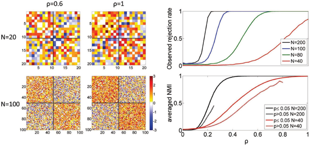
To evaluate the sensitivity of our test (probability of detecting a true modular structure), we gradually introduced a 2-cluster structure to a Gaussian random network by combining two adjacency matrices with a scaling constant: A = G + ρS, where G is the adjacency matrix of a Gaussian random network with edges following a standard normal distribution, S is the adjacency matrix of a graph with two equal-size completed subgraphs (block diagonal matrix with weights 1 in the main diagonal blocks), and ρ ∈ [0, 1].
The simulated graphs are exemplified in Figure 8 (left), with a 2-cluster structure that is easier to discern when N is large. The observed rejection rate is plotted in Figure 8 (top right) as a function of N and ρ. For large N, the observed rejection rate is equal to the nominal 5% when ρ = 0, and rapidly approaches 1 as ρ increases. For small N (N < 80), sensitivity drops and the structure is more difficult to detect. To evaluate whether the rejection of the null hypotheses (and therefore the detection of graph structure) also leads to accurate partition results, we assess the overall similarity between the resulting and the correct partitions using normalized mutual information (NMI, Dhillon et al. (2004); Danon et al. (2005); Chang et al. (2012)). Figure 8 (bottom right) shows the average NMI for the graphs with detected structure (p ≤ 0.05; solid lines). For the graphs without a detected structure (p > 0.05; dashed lines), should we have proceeded with a partition, their average NMI would be considerably lower than the graphs with detected structure.
Figure 8.
(Left) Realizations of structured networks of size N = 20 and N = 100, with weights ρ = 0.6 and ρ = 1.(Top right) Rejection rate of the significance test on gradually introduced structured networks controlled by parameter ρ. (Bottom right) The averaged NMI of each clustering result against the true structure for p ≤ 0.05 and p > 0.05 for network size N = 40 and N = 200, respectively.
3.4. Modular Structure of Brain Connectomes
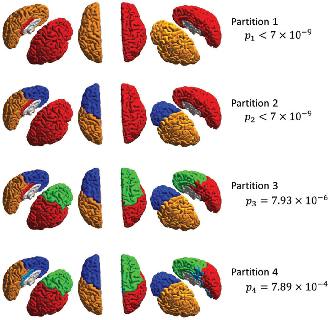
We applied our significance-based modularity partitioning to the structural brain network reported in Hagmann et al. (2008b). The network consists of 66 nodes representing FreeSurfer parcellated cortical regions and edges representing the neuronal fiber densities between pairs of regions. We reported partition results of this network in (Chang et al. (2012)), and now using our statistical method we confirm that all bi-partitions leading to 5 clusters are indeed significant with very small p-values (Figure 9). The structural data reveal subnetworks that largely conform to the classical lobe-based partitioning of the cerebral cortex.
Figure 9.
Modularity-based partitioning of the structural brain network in Hagmann et al. (2008b). Each color represents a different subnetwork. All clusters are statistically significant.
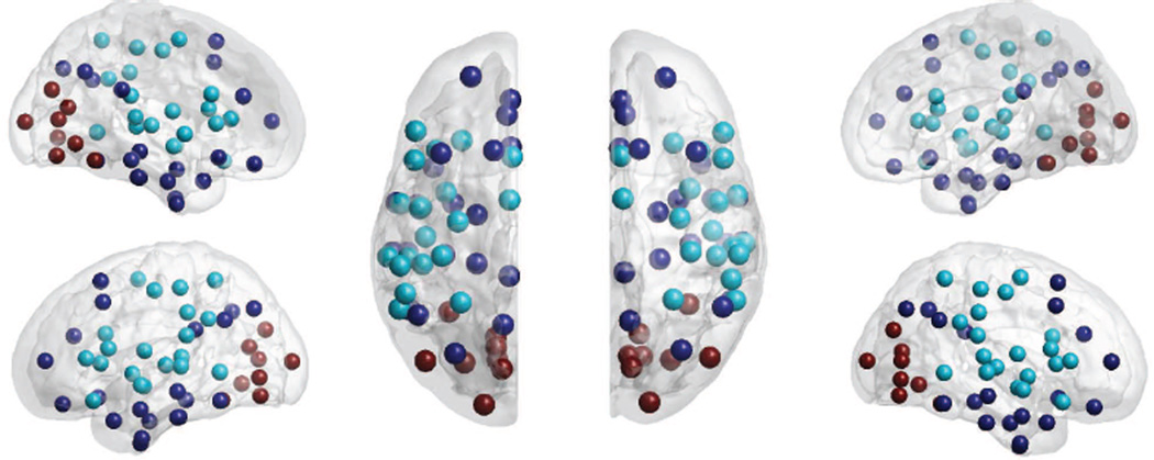
We also investigated the partitions of a brain network extracted from resting state fMRI data (Fox et al. (2005)). The data consists of 191 subjects from the Beijing data set of the 1000 Functional Connectomes Project in NITRC (Kelly et al. (2011)). The 96 nodes represent ROIs defined on the Harvard-Oxford atlas (Frazier et al. (2005); Makris et al. (2006)) and edges indicate the correlation coefficient between resting fMRI signals for each pair of ROIs. Correlations were computed after bandpass filtering in the range 0.005–0.1Hz. Following two sequential bi-partitions, both with p-value p < 7×10⁻¹⁰, we detected 3 clusters: the default mode network (task-negative network), a motor-sensory subnetwork (task-positive network), and a visual-related subnetwork. The functional subnetworks involve large scale interactions and follow well known functional sub-divisions (Fox et al. (2005)).
The above results were also confirmed with a conventional resampling approach. By generating 105 Gaussian random networks with edges having equal mean and variance as the original fMRI network, the same bi-partitions were significant with p-value p < 10−5. However, the resampling approach required a thousand-fold more computational time, highlighting the effectiveness of our parametric approach.
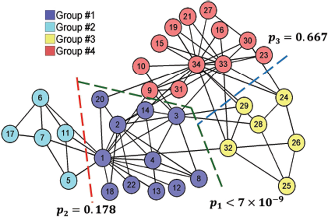
Finally, we partitioned the widely-studied Karate Club network in Zachary (1977) shown in Figure 11. Three sequential bi-partitions were obtained by the modularity algorithm: first separating groups {1, 2} from {3, 4}, and then {1} from {2}, and {3} from {4}. The corresponding p-values for each bi-partition are also shown in Figure 11. The first bi-partition is significant and correctly predicts the actual split of the Karate club into two groups after a fight within its members. The rest of the bi-partitions are not significant.
Figure 11.
Partitions of the Karate Club network Zachary (1977).
4. Discussion
Modularity algorithms use the spectral decomposition of matrix B, the difference between the original and the null network, to partition a graph. Subtracting these two networks introduces dependencies across the elements of B, preventing the direct application of Tracy-Widom mapping for the estimation of the distribution of the maximum eigenvalue of B. However, our choice of power functions (Equations (7) and (8)), inspired by the Tracy-Widom mapping of the Gaussian orthogonal ensembles (Equation (5)), resulted in a very precise numerical fit. In fact, the parameter w2 has constants α2 and β2 with values very close to the original Tracy-Widom mapping (i.e. α2 ≈ −2 and β2 ≈ 2/3). This is not a coincidence, but rather indicates that the Tracy-Widom mapping may potentially be extended to matrices with across-element dependencies. In this paper we did not provide a theoretical derivation for the mappings in Equations (7) and (8). A theoretical derivation is not easy and beyond the scope of this paper.
To perform clustering, we sequentially bi-partition networks as in (Chang et al. (2012)). An alternative would be to use multiple eigenvectors to directly identify multiple clusters (Von Luxburg (2007); Van Mieghem (2011)). Although such method may provide better partitions, it requires prior knowledge of the number of clusters and can also not guarantee to a global optimum of modularity due to the NP-hard clustering problem. In addition, it demands a more complex model for the joint distribution of multiple eigenvalues to assess the significance of community structures, and our approach does not readily generalize to such a partition scheme.
The time complexity of our Monte-Carlo simulations reflects the nature of spectral decomposition of a network and is O(mN3) to perform spectral decomposition of m random networks of size N (Hu et al. (2010); Von Luxburg (2007)). Practically, our 64-bit 12-core-2.67GHz-processor with multi-threading machine requires 88 seconds to complete m = 105 simulations for N = 25, 198 seconds for N = 100 and 2534 seconds (≈ 42 minutes) for N = 500.
Depending on the fine-tuning algorithms following the spectral partitions, conventional methods, either based on perturbation or randomization, share time complexity no less than O(mN3), given that testing a single network requires generating m realizations of random networks. In contrast, the time complexity of evaluating significance of the modular structures using our method is only O(1) and the computational time is negligible.
Given the precision of the fitting results, we are confident that the form of our mapping is accurate. However, a better estimation of the parameters listed in Table 1 is certainly feasible by a) expanding our Monte Carlo simulations, and b) performing alternative numerical optimization procedures. In particular, computing more network realizations, especially with higher network sizes, will produce more accurate estimates of functions w1 and w2. Furthermore, our numerical optimization independently fit w1 and w2 functions; a joint optimization could lead to a more accurate estimation of the parameters in Table 1, however our implementations were prone to local minima and did not achieve stable results.
Our two stage formulas control error rate reasonably well over network sizes N up to 6000−8000; at N = 8000 the test becomes liberal and achieves approximately 8% rather than 5% Type I error rate. We do not recommend applying the statistical test beyond this range. However, refining the estimation of parameters in Table 1 should broaden the range where the test becomes specific (Type I error rate equal to nominal). We conjecture that the form of the power functions for w1 and w2 will remain unchanged, and only a better estimation of the parameters in Table 1 is required.
Our empirical formulas are applicable only for modularity partitioning that uses as a null model the conditional expected network in equation (2) (Chang et al. (2012)). For the case of the conventional null model in equation (1) proposed by Newman and Girvan (2004), our simulations (not included in this paper) indicate that the distribution of the maximum eigenvalue of matrix BRandom can still be described by a linearly transformed Tracy-Widom distribution. However, this distribution is a function of not only N and σ2, but also the edge mean μ (Figure 2). Therefore, the power functions in equations (7) and (8) are no longer suitable and more complex functions are necessary to approximate such a distribution.
Assume a network A with edges following a Gaussian distribution with standard deviation equal to σ. We can write the eigenvalue decomposition of the difference matrix B with eigenvalues in the diagonal matrix D and eigenvectors in E:
Therefore, if network A is normalized to A/σ (thus edges having unit standard deviation), the difference matrix B is similarly scaled as B/σ. This implies that the scaled network A/σ has the same partition results (eigenvectors E remain unchanged) but eigenvalues are weighted by 1/σ, justifying the correction found in equation (7).
An alternative approach to using the Tracy-Widom distribution would be to seek parametric formulas based on the Gamma distribution. It has been shown that scaled and shifted Gamma distributions can well approximate the Tracy-Widom distribution, either by directly minimizing the difference between the two distributions (Vlok and Olivier (2012)), or by matching their first, second, and third moments (Wei and Tirkkonen (2011); Chiani (2012)). In (Chang et al. (2013)) we showed that such an approach led to inferior numerical results than the Tracy-Widom distribution.
5. Conclusions
Motivated by the Tracy-Widom mapping in random matrix theory, we have provided empirical formulas that parametrically model the null distribution of modularity for any network of size N and jointly Gaussian distribution of edges with mean mu and standard deviation sigma. Our approach allows statistical tests for modularity-based network partitions without the need of computationally expensive resampling procedures of individual networks. We have shown that type I error rate is controlled efficiently for large networks up to 8, 000 nodes, and with more extensive and accurate numerical simulations, we postulate that our formulas can be refined to control error rate to arbitrarily large networks.
Figure 10.
Partition results of a resting state fMRI network. All 3 clusters, indicated by the color of the spheres, are significant.
Highlights.
We prove that the distribution of brain modules follows a modified Tracy-Widom distribution
We construct parametric formulas that predict the distribution of brain modules
A Monte-Carlo simulation estimates the model parameters
Our method provides formal statistical inference in brain networks
Acknowledgements
This work supported by the National Institutes of Health under grants R01-EB000473(NIBIB), R01-EB009048(NIBIB), and the National Science Foundation under grant BCS-1134780.
Appendix A
Introduction to the Tracy-Widom Distribution
Tracy and Widom (Tracy and Widom (2000)) derived analytical solutions for the distribution of the largest eigenvalue of three types of random matrices Gβ: the Gaussian Orthogonal Ensembles (real symmetric matrices, GOE, β = 1), the Gaussian Unitary Ensembles (hermitian matrices, GUE, β = 2), and the Gaussian Symplectic Ensembles (self-dual matrices, GSE, β = 4):
| (A.1) |
| (A.2) |
| (A.3) |
where A1 is N × N with real elements following an i.i.d. (𝒩0, 2σ2) normal distribution, A2 is N × N with complex elements whose real and imaginary parts follow an i.i.d. 𝒩(0, σ2) normal distribution, ()D denotes the self transpose of a quaternion matrix, and A4 is 2N × 2N obtained from:
where X and Y are two independent realizations of A2 of size N × N. The standard deviation of the off-diagonal elements of all matrices G1, G2 and G4 is σ. Of special interest to modularity-based partitioning is the GOE case, because undirected networks have real and symmetric adjacency matrices.
Let T = λ1(Gβ) be a random variable equal to the largest eigenvalue λ1 of any of the above random ensembles. Tracy and Widom (Tracy and Widom (2000)) derived an important scaling formula that predicts the distribution of T :
| (A.4) |
where
| (A.5) |
and S follows the Tracy-Widom distributions below. Note, that β = 2 is the simplest case and is used to derive the other cases:
| (A.6) |
| (A.7) |
| (A.8) |
were q is the solution to the Painlevé II equation: q′′ = sq + 2q3, satisfying the condition q(s) ≈ Ai(s) as s → ∞, with Ai the Airy function (Tracy and Widom (2000)).
Using equation (A.4), we can derive the distribution of the largest eigenvalue for any Gaussian ensemble for different values of N and σ.
Footnotes
Publisher's Disclaimer: This is a PDF file of an unedited manuscript that has been accepted for publication. As a service to our customers we are providing this early version of the manuscript. The manuscript will undergo copyediting, typesetting, and review of the resulting proof before it is published in its final citable form. Please note that during the production process errors may be discovered which could affect the content, and all legal disclaimers that apply to the journal pertain.
References
- Alexander-Bloch A, Gogtay N, Meunier D, Birn R, Clasen L, Lalonde F, Lenroot R, Giedd J, Bullmore E. Disrupted modularity and local connectivity of brain functional networks in childhood-onset schizophrenia. Frontiers in systems neuroscience. 2010;4 doi: 10.3389/fnsys.2010.00147. [DOI] [PMC free article] [PubMed] [Google Scholar]
- Bassett DS, Bullmore E. Small-world brain networks. The neuroscientist. 2006;12(6):512–523. doi: 10.1177/1073858406293182. [DOI] [PubMed] [Google Scholar]
- Bullmore E, Bassett D. Brain graphs: graphical models of the human brain connectome. Annual review of clinical psychology. 2011;7:113–140. doi: 10.1146/annurev-clinpsy-040510-143934. [DOI] [PubMed] [Google Scholar]
- Bullmore E, Sporns O. Complex brain networks: graph theoretical analysis of structural and functional systems. Nature Reviews Neuroscience. 2009;10(3):186–198. doi: 10.1038/nrn2575. [DOI] [PubMed] [Google Scholar]
- Chang Y, Leahy R, Pantazis D. Modularity-based graph partitioning using conditional expected models. Physical Review E. 2012;85(1):016109. doi: 10.1103/PhysRevE.85.016109. [DOI] [PMC free article] [PubMed] [Google Scholar]
- Chang Y, Leahy R, Pantazis D. Biomedical Imaging: From Nano to Macro, 2013 IEEE International Symposium on. IEEE; 2013. Parametric distributions for assessing significance in modular partitions of brain networks; pp. 612–615. [Google Scholar]
- Chavez M, Valencia M, Navarro V, Latora V, Martinerie J. Functional modularity of background activities in normal and epileptic brain networks. Physical review letters. 2010;104(11):118701. doi: 10.1103/PhysRevLett.104.118701. [DOI] [PubMed] [Google Scholar]
- Chen Z, He Y, Rosa-Neto P, Gong G, Evans A. Age-related alterations in the modular organization of structural cortical network by using cortical thickness from mri. NeuroImage. 2011;56(1):235–245. doi: 10.1016/j.neuroimage.2011.01.010. [DOI] [PubMed] [Google Scholar]
- Chiani M. Distribution of the largest eigenvalue for real wishart and gaussian random matrices and a simple approximation for the tracy-widom distribution. arXiv preprint arXiv: 1209.3394. 2012 [Google Scholar]
- Danon L, Díaz-Guilera A, Duch J, Arenas A. Comparing community structure identification. Journal of Statistical Mechanics: Theory and Experiment 2005. 2005:P09008. [Google Scholar]
- Dhillon I, Guan Y, Kulis B. Proceedings of the tenth ACM SIGKDD international conference on Knowledge discovery and data mining. ACM; 2004. Kernel k-means: spectral clustering and normalized cuts; pp. 551–556. [Google Scholar]
- Dimitriadis S, Laskaris N, Tsirka V, Vourkas M, Micheloyannis S, Fotopoulos S. Tracking brain dynamics via time-dependent network analysis. Journal of neuroscience methods. 2010;193(1):145–155. doi: 10.1016/j.jneumeth.2010.08.027. [DOI] [PubMed] [Google Scholar]
- Edelman A, Rao N. Random matrix theory. Acta Numerica. 2005;14(1):233–297. [Google Scholar]
- Erdős P, Rényi A. On the evolution of random graphs. Magyar Tud. Akad. Mat. Kutató Int. Közl. 1960;5:17–61. [Google Scholar]
- Fan Y, Shi F, Smith J, Lin W, Gilmore J, Shen D. Brain anatomical networks in early human brain development. Neuroimage. 2011;54(3):1862–1871. doi: 10.1016/j.neuroimage.2010.07.025. [DOI] [PMC free article] [PubMed] [Google Scholar]
- Fox M, Snyder A, Vincent J, Corbetta M, Van Essen D, Raichle M. The human brain is intrinsically organized into dynamic, anticorrelated functional networks. Proceedings of the National Academy of Sciences of the United States of America. 2005;102(27):9673. doi: 10.1073/pnas.0504136102. [DOI] [PMC free article] [PubMed] [Google Scholar]
- Frazier JA, Chiu S, Breeze JL, Makris N, Lange N, Kennedy DN, Herbert MR, Bent EK, Koneru VK, Dieterich ME, et al. Structural brain magnetic resonance imaging of limbic and thalamic volumes in pediatric bipolar disorder. American Journal of Psychiatry. 2005;162(7):1256–1265. doi: 10.1176/appi.ajp.162.7.1256. [DOI] [PubMed] [Google Scholar]
- Gómez S, Jensen P, Arenas A. Analysis of community structure in networks of correlated data. Physical Review E. 2009;80(1):016114. doi: 10.1103/PhysRevE.80.016114. [DOI] [PubMed] [Google Scholar]
- Guimerá R, Sales-Pardo M, Amaral L. Modularity from fluctuations in random graphs and complex networks. Phys. Rev. E. 2004;70(2):025101. doi: 10.1103/PhysRevE.70.025101. [DOI] [PMC free article] [PubMed] [Google Scholar]
- Hagmann P, Cammoun L, Gigandet X, Meuli R, Honey C, Wedeen V, Sporns O. Mapping the structural core of human cerebral cortex. PLoS biology. 2008b;6(7):e159. doi: 10.1371/journal.pbio.0060159. [DOI] [PMC free article] [PubMed] [Google Scholar]
- Hagmann P, Cammoun L, Gigandet X, Meuli R, Honey C, Wedeen V, Sporns O. Mapping the structural core of human cerebral cortex. PLoS biology. 2008b;6(7):e159. doi: 10.1371/journal.pbio.0060159. [DOI] [PMC free article] [PubMed] [Google Scholar]
- He Y, Wang J, Wang L, Chen Z, Yan C, Yang H, Tang H, Zhu C, Gong Q, Zang Y, et al. Uncovering intrinsic modular organization of spontaneous brain activity in humans. PLoS One. 2009;4(4):e5226. doi: 10.1371/journal.pone.0005226. [DOI] [PMC free article] [PubMed] [Google Scholar]
- Hochberg Y, Tamhane AC. Multiple comparison procedures. John Wiley & Sons, Inc; 1987. [Google Scholar]
- Hu Y, Nie Y, Yang H, Cheng J, Fan Y, Di Z. Measuring the significance of community structure in complex networks. Physical Review E. 2010;82(6):066106. doi: 10.1103/PhysRevE.82.066106. [DOI] [PubMed] [Google Scholar]
- Johansson K. Shape fluctuations and random matrices. Communications in Mathematical Physics. 2000;209:437–476. [Google Scholar]
- Johnstone I. On the distribution of the largest eigenvalue in principal components analysis.(english. Ann. Statist. 2001;29(2):295–327. [Google Scholar]
- Karrer B, Levina E, Newman M. Robustness of community structure in networks. Physical Review E. 2008;77(4):046119. doi: 10.1103/PhysRevE.77.046119. [DOI] [PubMed] [Google Scholar]
- Kelly C, Shehzad Z, Mennes M, Milham M. Functional connectome processing scripts. 2011 http://www.nitrc.org/projects/fcon_1000.
- Lancichinetti A, Radicchi F, Ramasco J. Statistical significance of communities in networks. Physical Review E. 2010;81(4):046110. doi: 10.1103/PhysRevE.81.046110. [DOI] [PubMed] [Google Scholar]
- Makris N, Goldstein JM, Kennedy D, Hodge SM, Caviness VS, Faraone SV, Tsuang MT, Seidman LJ. Decreased volume of left and total anterior insular lobule in schizophrenia. Schizophrenia research. 2006;83(2):155–171. doi: 10.1016/j.schres.2005.11.020. [DOI] [PubMed] [Google Scholar]
- Maslov S, Sneppen K. Specificity and stability in topology of protein networks. Science. 2002;296(5569):910. doi: 10.1126/science.1065103. [DOI] [PubMed] [Google Scholar]
- Meunier D, Lambiotte R, Bullmore E. Modular and hierarchically modular organization of brain networks. Frontiers in neuroscience. 2010;4 doi: 10.3389/fnins.2010.00200. article 200. [DOI] [PMC free article] [PubMed] [Google Scholar]
- Meunier D, Lambiotte R, Fornito A, Ersche K, Bullmore E. Hierarchical modularity in human brain functional networks. Frontiers in neuroinformatics. 2009;3(37) doi: 10.3389/neuro.11.037.2009. [DOI] [PMC free article] [PubMed] [Google Scholar]
- Mirshahvalad A, Beauchesne OH, Archambault É, Rosvall M. Resampling effects on significance analysis of network clustering and ranking. PloS one. 2013;8(1):e53943. doi: 10.1371/journal.pone.0053943. [DOI] [PMC free article] [PubMed] [Google Scholar]
- Mirshahvalad A, Lindholm J, Derlén M, Rosvall M. Significant communities in large sparse networks. PloS one. 2012;7(3):e33721. doi: 10.1371/journal.pone.0033721. [DOI] [PMC free article] [PubMed] [Google Scholar]
- Newman M. Modularity and community structure in networks. Proceedings of the National Academy of Sciences. 2006;103(23):8577. doi: 10.1073/pnas.0601602103. [DOI] [PMC free article] [PubMed] [Google Scholar]
- Newman M, Girvan M. Finding and evaluating community structure in networks. Physical review E. 2004;69(2):026113. doi: 10.1103/PhysRevE.69.026113. [DOI] [PubMed] [Google Scholar]
- Nichols T, Hayasaka S. Controlling the familywise error rate in functional neuroimaging: a comparative review. Statistical methods in medical research. 2003;12(5):419–446. doi: 10.1191/0962280203sm341ra. [DOI] [PubMed] [Google Scholar]
- Reichardt J, Bornholdt S. When are networks truly modular? Physica D: Nonlinear Phenomena. 2006;224(1):20–26. [Google Scholar]
- Reichardt J, Bornholdt S. Partitioning and modularity of graphs with arbitrary degree distribution. Physical Review E. 2007;76(1):015102. doi: 10.1103/PhysRevE.76.015102. [DOI] [PubMed] [Google Scholar]
- Rubinov M, Sporns O. Complex network measures of brain connectivity: uses and interpretations. Neuroimage. 2010;52(3):1059–1069. doi: 10.1016/j.neuroimage.2009.10.003. [DOI] [PubMed] [Google Scholar]
- Rudie J, Brown J, Beck-Pancer D, Hernandez L, Dennis E, Thompson P, Bookheimer S, Dapretto M. Altered functional and structural brain network organization in autism. NeuroImage: Clinical. 2013;2:77–94. doi: 10.1016/j.nicl.2012.11.006. [DOI] [PMC free article] [PubMed] [Google Scholar]
- Salvador R, Suckling J, Coleman M, Pickard J, Menon D, Bullmore E. Neurophysiological architecture of functional magnetic resonance images of human brain. Cerebral Cortex. 2005;15(9):1332–1342. doi: 10.1093/cercor/bhi016. [DOI] [PubMed] [Google Scholar]
- Seifi M, Junier I, Rouquier J-B, Iskrov S, Guillaume J-L. Stable community cores in complex networks. Complex Networks. 2012:87–98. [Google Scholar]
- Singh AK, Phillips S. Hierarchical control of false discovery rate for phase locking measures of eeg synchrony. NeuroImage. 2010;50(1):40–47. doi: 10.1016/j.neuroimage.2009.12.030. [DOI] [PubMed] [Google Scholar]
- Sporns O, Honey C, Kötter R. Identification and classification of hubs in brain networks. PLoS One. 2007;2(10):e1049. doi: 10.1371/journal.pone.0001049. [DOI] [PMC free article] [PubMed] [Google Scholar]
- Tao T. Topics in random matrix theory. Amer Mathematical Society. 2012;Vol. 132 [Google Scholar]
- Tomasi D, Volkow N. Functional connectivity hubs in the human brain. Neuroimage. 2011;57(3):908–917. doi: 10.1016/j.neuroimage.2011.05.024. [DOI] [PMC free article] [PubMed] [Google Scholar]
- Tracy C, Widom H. The distribution of the largest eigenvalue in the gaussian ensembles. Calogero-Moser-Sutherland Models, CRM Series in Mathematical Physics. 2000;4:461–472. [Google Scholar]
- Vaessen M, Hofman P, Tijssen H, Aldenkamp A, Jansen J, Backes W. The effect and reproducibility of different clinical dti gradient sets on small world brain connectivity measures. Neuroimage. 2010;51(3):1106–1116. doi: 10.1016/j.neuroimage.2010.03.011. [DOI] [PubMed] [Google Scholar]
- Van den Heuvel M, Stam C, Boersma M, Hulshoff Pol H. Small-world and scale-free organization of voxel-based resting-state functional connectivity in the human brain. Neuroimage. 2008;43(3):528–539. doi: 10.1016/j.neuroimage.2008.08.010. [DOI] [PubMed] [Google Scholar]
- Van Mieghem P. Graph Spectra for Complex Networks. Cambridge University Press; 2011. [Google Scholar]
- Vlok J, Olivier J. Analytic approximation to the largest eigenvalue distribution of a white wishart matrix. Communications, IET. 2012;6(12):1804–1811. [Google Scholar]
- Von Luxburg U. A tutorial on spectral clustering. Statistics and Computing. 2007;17(4):395–416. URL http://www.kyb.mpg.de/fileadmin/user_upload/files/publications/attachments/Luxburg07_tutorial_4488%5b0%5d.pdf. [Google Scholar]
- Wang Q, Su T, Zhou Y, Chou K, Chen I, Jiang T, Lin C, et al. Anatomical insights into disrupted small-world networks in schizophrenia. NeuroImage. 2012;59(2):1085–1093. doi: 10.1016/j.neuroimage.2011.09.035. [DOI] [PubMed] [Google Scholar]
- Wei L, Tirkkonen O. Communications (ICC), 2011 IEEE International Conference on. IEEE; 2011. Analysis of scaled largest eigenvalue based detection for spectrum sensing; pp. 1–5. [Google Scholar]
- Yekutieli D, Reiner-Benaim A, Benjamini Y, Elmer G, Kafkafi N, Letwin N, Lee N. Approaches to multiplicity issues in complex research in microarray analysis. Statistica Neerlandica. 2006;60(4):414–437. [Google Scholar]
- Zachary W. An information flow model for conflict and fission in small groups. Journal of anthropological research. 1977;33:452–473. [Google Scholar]


