

Abstract
Purpose: Kilovoltage cone-beam computed tomography (CBCT) is widely used in image-guided radiation therapy for exact patient positioning prior to the treatment. However, producing time series of volumetric images (4D CBCT) of moving anatomical structures remains challenging. The presented work introduces a novel method, combining high temporal resolution inside anatomical regions with strong motion and image quality improvement in regions with little motion.
Methods: In the proposed method, the projections are divided into regions that are subject to motion and regions at rest. The latter ones will be shared among phase bins, leading thus to an overall reduction in artifacts and noise. An algorithm based on the concept of optical flow was developed to analyze motion-induced changes between projections. The technique was optimized to distinguish patient motion and motion deriving from gantry rotation. The effectiveness of the method is shown in numerical simulations and patient data.
Results: The images reconstructed from the presented method yield an almost the same temporal resolution in the moving volume segments as a conventional phase-correlated reconstruction, while reducing the noise in the motionless regions down to the level of a standard reconstruction without phase correlation. The proposed simple motion segmentation scheme is yet limited to rotation speeds of less than .
Conclusions: The method reduces the noise in the reconstruction and increases the image quality. More data are introduced for each phase-correlated reconstruction, and therefore the applied dose is used more efficiently.
Keywords: cone-beam CT (CBCT), 4D CBCT, AAPC
INTRODUCTION
The use of kV cone-beam computed tomography (CBCT) devices mounted on linear particle accelerators (LINACs) for image-guided radiation therapy has introduced new possibilities for a more precise patient positioning.1 In the future, kV CBCT images may become the basis to adapt radiation therapy plans during the course of the treatment. Images acquired with the CBCT device can be registered to the images of a reference CT used for planning. The megavoltage beam is adopted to the possible organ displacement and the irradiation of sound tissue is reduced. A common application for 4D images, therefore, is the planning for the treatment of lung cancer as one has the cyclic respiratory motion in the thoracic region.
The main disadvantage of CBCT mounted on radiation therapy gantries compared to clinical CT scanners is the slow rotation speed, which is limited by safety reasons to typically . The high rotation velocity of clinical CT scanners of less than makes it possible to avoid artifacts from respiratory motion by making the patient hold his breath for the short scan duration. This approach is not feasible for the LINAC-mounted units where the smallest possible scan duration is about for a -angle scan.2 Instead, the algorithms for 4D CBCT reconstruction have to deal with motion within the dataset. Using the standard reconstruction on a motion contaminated dataset results in motion artifact, which are shown, for example, for a mathematical phantom and patient images in Fig. 1. The simplest way of reconstructing motion affected projections from slow rotation CBCT units is to assume a cyclic motion and to estimate the motion phase for each projection. This can be done, e.g., by using the Varian (Palo Alto, CA) real-time position management system, detecting the motion phase from the patient’s thorax. Then the projections are sorted to nearly motion-free subsets of motion phases with sizes of, e.g., , and reconstructed with standard methods like the filtered backprojection (FBP) algorithm from Feldkamp, Davis, and Kress (FDK).3
Figure 1.

Standard reconstruction: Motionless phantom (upper left) and patient image (lower left), phantom with motion of ellipsoids and inserts (upper right) and patient image with respiratory motion artifacts (lower right). The arrows point to moving and therefore blurred tissue. Also, streak artifacts are visible (, ).
There have been several publications using this method with on-board imager (OBI) units, which are part of the Varian LINACs.4, 5, 6, 7 Although being relatively simple, the approach has the major drawback of introducing streak artifacts due to the low number of projections effectively used for the reconstruction of each motion phase. Also the noise is enhanced to a large degree as less projection information is available.
Nevertheless, there are also reconstruction schemes that try to avoid artifacts and instead reconstruct images by combining data from several rotations to a single scan with a high temporal resolution. One of the first approaches was that in Ref. 8 with the application for ECG-gated cardiac imaging with a clinical CT system. Recently, there are also approaches with C-arm CT devices like that in Ref. 9. These approaches apply a weight to each projection depending on their motion phase. Combining and normalizing the weighted projections for each angular position to a single one always yields a valid projection, although the temporal resolution in this projection can vary.
In Ref. 10 the possibility was analyzed to also acquire the necessary data in several rotations with an OBI unit. Although the number of rotation is restricted by the overall scan duration, it still can be an option for 4D CBCT with LINAC mounted kV units. The only restrictions lie in the mechanical components, i.e., the acceleration and deceleration of the large gantry, as well as the possibility to gate the start of the rotation or the radiation.2
Besides the phase-correlated methods, there are also motion-compensation methods that use all projections and a deformation map to compensate for the motion.1, 11, 12 The deformation map can be calculated from the planning CT and the assumption is made that the intrafraction motion during the treatment sessions remains almost unchanged. Motion-compensated algorithms naturally have a higher computational effort than the phase-correlated methods. This includes the calculation of the deformation, the matching of the geometry of the CBCT and the planning CT, and also the reconstruction. The latter is usually much slower when a deformed geometry has to be included. Nevertheless, there are approaches11 to speed up the motion compensation during the backprojection, which enables the clinical usage of such methods. Possible misregistrations of the geometries of the planning CT and the CBCT and inaccuracies in the calculated deformations are additional problems that have to be faced with motion-compensating algorithms.
The algorithm that is proposed here does not compensate the motion but will only introduce a phase-correlated detector pixel weighting. Thus, this approach is simpler and relies on the CBCT raw data only. There is no need for additional prior information as well as additional computation with respect to the planning CT. Inaccuracies regarding the geometries or deformations do not play a role. Due to the reduced projection information that is used for the reconstruction of each motion cycle, one usually has to face higher artifact and noise levels.
The previously introduced 4D phase-correlated reconstruction schemes all do a projectionwise phase-dependent weighting, which also includes projection regions being motionless and not being in need of this weighting at all. The introduction of these regions to the reconstruction process will reduce the noise in the motionless voxel and keep the temporal resolution as high as in the conventional approaches. This is accomplished by the new autoadaptive phases-correlation (AAPC) algorithm that will be described in the following sections. The main purpose of the proposed reconstruction scheme is to maximize the dose usage in 4D CBCT. The dose and the corresponding projection information not being used by the conventional phase-correlated reconstruction are here used to reduce streak artifacts from motionless high contrast objects like bones. The motionless outer anatomy of the patient is more clearly delineated. On the one hand, this is positive for the subjective visual aspects and, on the other hand, registration algorithms being applied to the image will profit, as the image incorporates less noise and artifacts.
While improving the image quality of motionless tissue, the algorithm does not affect the phase-correlated reconstruction of the moving parts. For this problem, additional information or additional calculations like iterative reconstructions would be necessary, which would introduce a significant latency to the workflow. The proposed algorithm works on the projection data only and has almost no additional latency. The reconstruction algorithm is preceded by a motion detection that estimates and segments the motion affected areas within the projection and then yields a projection pixel weighting. For the reconstruction, the extended parallel backprojection (EPBP) algorithm13 is used, which is adapted to the flat detector geometry. This type of algorithm is necessary as the weighting will be individual for each volume voxel. The algorithm is further modified to be able to deal with nonzero and zero weights, i.e., the hard exclusion of pixel to the reconstruction.
In order to validate this approach, the AAPC algorithm is compared to a conventional phase-correlated reconstruction with a weighting of the whole projection and the conventional non-phase-correlated reconstruction. Reconstructions from a mathematical phantom as well as reconstructed patient data are shown.
MATERIALS AND METHODS
As already mentioned, the main purpose of the reconstruction scheme is to maximize the dose usage in 4D CBCT by distinguishing between areas in projections requiring a phase-correlated weighting and those being motionless. The motion-detection algorithm is assumed to give a segmentation for motion affected areas within each projection. Combining the segmented areas with a motion-phase-dependent weight yields a projection pixel weighting to each projection with u and v being the coordinates on the two-dimensional detector and α being the projection angle on the circular trajectory. Both, the weighting and the projections, can then be fed into a suitable reconstruction algorithm being able to deal with these pixel-dependent weightings.
Motion detection and weighting
The AAPC reconstruction includes a preprocessing that detects the motion within the projections. It is accomplished by applying the so-called optical flow algorithms on consecutive projections. Most common optical flow methods are based on the assumption that pixel intensities do not change, see e.g., Refs. 14, 15. Nevertheless, one can also derive them from the continuity equation
stating that the total attenuation on the detector is preserved under the influence of the motion over the time if there is no additional attenuation created or removed within the projected volume. Here, and are the pixel velocities in the corresponding directions and p are the projections. These kind of equations is broadly used for continuity modeling in many application domains as, for instance, in electromagnetic field theory, where it can be used to express the conservation of charge.
Although there are truncated projections for most scans with the OBI scanner as the detector with size of in most cases is too small to cover the projection image of the whole object, the continuity equation will approximately be locally valid between two projections as one has attenuation contributions that enter and leave the projection from at the edges of the detector.
Rewriting this equation yields
Also, assuming that the derivative of the motion vectors in the corresponding directions is negligibly small, one obtains
This approximation is used here to employ efficient algorithms from the computation of optical flow as the base equation is the same there. The Horn–Schunk15 is used for AAPC as it is simple and yields dense motion vector fields,16 which is favorable for a segmentation. For two projections, the algorithm gives an estimate for the velocity of attenuation values on the detector.
In the subsequent segmentation process, an image will be regarded as motionless when the velocity of a pixel has constantly the same direction in a certain observation range. In this case, a projection and its two neighboring projection are observed. As one has to take into account the possible displacement of the pixel due to the system rotation, all possible displacements that can take place due to rotation are checked. Figure 2 illustrates the observation windows, e.g., a pixel can travel from the left border of the window at time step through the center at time step α to the right border at time step . If one finds a path through the center where a velocity in a single direction takes place, one can assume that the pixel is moving monotonically due to rotation. In the case of cyclic motion, one will have a change in direction in the motion which then will be detected. In order to be more robust to noise, only velocity values above a certain threshold are taken into account. These thresholds are empirically chosen to reduce the noise dependent fluctuations in projections with temporally unchanged attenuation values. The size of the observation window that is used can be estimated by calculating the worst case displacement of a pixel in the projection due to the system rotation. The worst case movement of pixel on the detector can be derived from the rotation of a voxel in the volume. The perspective mapping from the voxel to the projections is described as
| (1) |
| (2) |
with
| (3) |
with being the distance from the source to the detector and being the distance from the center of rotation to the source. The velocity of a pixel on the detector can be derived by taking the derivative with respect to α,
As the maximum velocity for any attenuation value on the detector is to be determined, one can use the worst case of , i.e., a pixel at the edge of the reconstruction region with radius . Assuming rotational invariance, one simply set in Eqs. 1, 2, 3 and insert the values so one receives
This quadratic equation can be solved for y. The lower solution for y is taken as it has a higher magnification on the detector. Using this solution, one gets the corresponding x and z coordinates of the voxel at the edge of the field of measurement. The coordinates can then be placed into the derivative of u and v with respect to α, which gives a worst case estimate for the velocity of a projected voxel on the detector where the voxel is placed at the edge of the field of measurement. The segmented areas for a single time step have to be combined in a temporal manner so that the information of a direction change in the velocity is also spread in the intermediate segmentations. The segmentations from a total period of approximately one motion cycle are therefore combined to a single one by declaring a pixel as motion affected when it is segmented as being motion affected in any projection within the motion cycle.
Figure 2.

Observation window for the segmentation of motionless areas. If a possible displacement within the cone can be found, then the pixel at the center is segmented as motionless.
Depending on the motion phase used for reconstruction, the segmented array is then weighted and mapped by the function . A possible weighting function is the selection of projection pixel belonging to a certain motion-phase window around the reconstruction phase only, i.e.,
with being the rectangular function
Reconstruction algorithm
The reconstruction is based on the EPBP algorithm.13 The algorithm does a rebinning to pseudoparallel geometry and is then able to weight the direct and complementary rays in multiples of 180° against each other. This is especially useful if these rays were acquired in different motion phases as the temporal resolution can be enhanced. In the centered slice, the algorithm is exact, while in the outer regions, cone-beam artifacts might appear, just as with the FDK algorithm, as no exact reconstruction is possible for the circle trajectory in CBCT in general.
The algorithm was modified for the case that projection pixel has too low weights. Such a scenario might occur, in particular, when a scan with only a single rotation is done and the phase-dependent weighting has to be applied. In such a case, one cannot avoid assuring a certain temporal resolution by excluding all rays with insufficient weights from the backprojection. Consequently, the missing projections have to be compensated in the reconstruction process. In the standard phase-correlated reconstruction missing projections, this compensation is done by applying an overall correction factor proportional to the reciprocal of backprojected rays to the reconstructed image in order approximate the correct CT numbers. For the AAPC method, an individual correction factor has to be calculated for each voxel, depending on the number of rays with sufficiently high weights which have been backprojected. However, this simple method has shown to introduce artifacts in the AAPC case as the numerical approximation of the backprojection integral with rectangular segments gets more incorrect when the summed samples are not distributed homogeneously. Therefore, the numerical approximation of the backprojection is done using a trapezoidal rule.17 This is equivalent to linear interpolating missing values in the integrand function of the backprojection integral for each single voxel. For a more detailed description of the reconstruction itself, refer to the Appendix0.
Simulated motion phantom
The simulations where carried out using a modified Thorax FORBILD phantom (www.imp.uni-erlangen.de/phantoms/thorax/4D_Thorax_Description.pdf). The phantom includes pseudorespiratory motion of the lungs. Also, the lungs contain small spherical inserts to evaluate the temporal resolution. Figure 3a shows the design of the phantom in transversal and coronal slices. The motion function [Fig. 3b] for the pseudorespiratory motion was derived from real motion data. The motion function is multiplied to all variable lengths and offsets of the moving objects inside the phantom, which are also indicated in Fig. 3a. The goal of our simulation study was to use the geometry of the Varian OBI system with and and a detector with a pixel spacing of . Simulations and reconstructions were carried out using a single 360° scan. The motion frequency was , while the rotation time for 360° was chosen to be . The number of projections for the scan was 1200. For the phase-correlated reconstruction, the reconstruction phase (peak exhale) was chosen.
Figure 3.
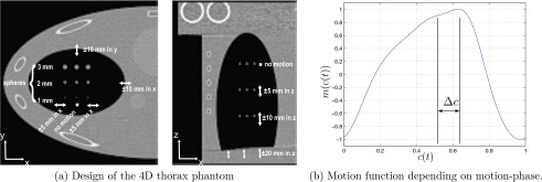
Overview over the 4D thorax phantom.
The noise model used for the evaluation was a Poisson distribution. The noiseless attenuated numbers of photons were transformed into Possion distributed values with mean and variance . The emitted number of quanta was chosen to .
Patient data
The patient dataset used for the evaluation of the AAPC reconstruction was “patient 3” from Ref. 4. The dataset consists of about 2000 projections over an angular range of approximately 200°, which is used for a short scan reconstruction over angle. The gantry rotation speed for the scan was , which corresponds to an overall scan time of . The detector frame rate was . The breathing cycle length of the patient during the scan was . The estimated dose, based on phantom dose measurements, was . The dataset has an intrinsic small angular sampling. Thus, phase-dependent weighting can be applied without introducing major streak artifacts. For this reconstruction, a rectangular weighting with an extent of the rectangle of 10% was chosen. The chosen reconstruction phase was the center of motion between exhale and inhale. The motion-phase information was extracted from the raw data from the center of mass of the projections. Such methods are well known from literature5, 18 and will not be discussed further.
Segmentation evaluation
In order to assess the performance of the proposed segmentation algorithm, the thorax phantom was simulated, varying the number of motion cycles over 360° , with being the motion frequency and being the rotation time. From the simulated data, the motion affected areas in the projections are known and used as the ground truth. The number of projections was held constant to 600 and also the simulated noise was held constant. Both combined correspond to a constant dose.
RESULTS
Segmentation evaluation
Figure 4 shows the results from the segmentation evaluation using a different number of motion cycles. Shown is the percentage of pixel that were unnecessarily segmented as motion affected as well as the percentage of pixel that were falsely segmented as motionless, although being motion affected. The latter will usually cause a degradation in the temporal resolution as well as motion artifacts. Also shown is the corresponding rotation speed assuming a scan over 360° and a motion frequency of .
Figure 4.

Evaluation of the segmentation performance for a varying number of motion cycles. The dashed line shows the percentage of pixel in the segmentation that was additionally marked as motion affected although being motionless. The dotted line shows the percentage of pixel that was falsely segmented as motionless, although being in the motion affected region. The black line shows the corresponding rotation speed for 360°, assuming a fixed motion frequency of . In the dashed region, the segmentation quality is degraded.
For less than 30 motion cycles (dashed area), a degradation of the segmentation can be observed. In this case the rotation is too fast so that gaps occur and motion affected areas are segmented as motionless. Moving objects in the projections are moved too far that in combination with other moving objects in the projection no smooth vector field can be found. For slower rotations and more motion cycles in 360°, i.e., , this error drops fast to a good coverage of all motion affected areas. In the segmentation process, one enlarges the initially segmented areas by a factor proportional to the possible rotation induced displacement of motion affected areas on the detector. Therefore, the areas that are segmented as motion affected are usually larger than the real motion affected areas on the detector. This fact is reflected in the false negative motion segmentation percentage with respect to the ground truth, i.e., the percentage of pixel that were unnecessarily marked as motion affected. This percentage drops for slower rotation speeds and in this case reaches a minimum of about 30%. This residual oversegmentation is mainly determined by the gap between the worst case displacement, which is used to enlarge the segmentation, and the real displacement of motion affected areas. The true moving regions within the volume are usually located more toward the inner volume and, consequently, have smaller displacements on the detector.
Phantom simulations
Figure 5 shows a single projection of the simulated phantom and the corresponding segmentation of motion affected areas (bright areas), in this case the lung ellipsoids. In Fig. 6 the reconstructed images are shown using the standard reconstruction, the conventional phase-correlated reconstruction, and the AAPC reconstruction. Also the difference images of the conventional phase-correlated reconstruction and the AAPC reconstruction are shown in order to compare the difference of temporal resolution in both. Regions of interest (ROIs) are placed at different locations within the phantom to evaluate the noise level in the different reconstructions.
Figure 5.

Projections for simulated dataset (left). The corresponding segmentations (right) for estimated motion affected regions are shown. A bright color indicates that the region will be subject to the phase-correlated weighting, while dark regions are used in each reconstruction phase.
Figure 6.

Reconstruction of various slices for the standard (Std), the conventional phase-correlated (PC), and the AAPC reconstruction for the slow 360° scan. Difference images of AAPC and conventional phase-correlated reconstructions are shown to distinguish the different levels of noise and the different temporal resolutions. ROIs are placed in various positions in motion affected and motionless regions in order to compare the image noise. The noise was calculated in difference images of two identical reconstructions with different noise realizations (images: , ), (difference image: , ).
The motion affected transversal slice includes motion from the lung and the sphere inserts. The standard images show blurred edges of the lung and also the spheres are blurred. The phase-correlated reconstructions instead have a higher contrast but still have a slight loss in CT numbers. The noise of the AAPC reconstruction in this slice tends more toward the conventional phase-correlated image. In the difference image, one can see no anatomical structures except the noise dependent ones, and in the inner lung, the temporal resolution of both images almost matches.
In the motionless transversal slice of the anthropomorphic phantom, the image noise of the AAPC reconstruction approaches the noise of the standard reconstruction, while in the motion affected slice, the noise in the AAPC image ( and ) is nearly as high as the noise in the image reconstructed with the conventional phase correlation ( and ). The overall noise level of the AAPC reconstructed images is lower than the one of the standard phase-correlated method.
Patient data
Figure 7 shows a transversal volume slice, which indicates the number of samples used for each voxel due to phase-correlated weighting (left image). The brighter, the more samples were used. If a rectangular integral approximation is used like for the conventional phase-correlated reconstruction, the images shows streak artifacts (middle image). Using a trapezoidal integral approximation solves this problem (right image). The images illustrate the necessity with this kind of compensation for the CT numbers in case that backprojection data are missing due to the specific pixel weighting.
Figure 7.

Slice with number of backprojected values (left, arbitrary units, and windowing). Reconstructed images using a simple integral approximation and AAPC (middle) and AAPC with the trapezoidal integral approximation (right) (, ).
Figure 8 show a single projection of the patient and the corresponding segmentation of motion affected areas (bright areas). In this case the tissue around the lung is detected to large degrees as motionless. Figure 9 presents the different reconstructions of the patient data. The transversal slice from the center of the volume shows almost the same temporal resolution in the two phase-correlated reconstructions. The difference image shows a low deviation between these two, especially in the inner lungs where most of the tissue is moving. The small mass at the left lung (arrow) is shown sharply and with high contrast in both images while there is a significant drop in intensity in the standard image where the mass is blurred due to motion. The good temporal resolution of is also visible in the other views. Only a slight anatomical mismatch on single ribs can be observed from the difference images. In the other regions, the difference images show differences in noise and no anatomical structures showing that the temporal resolution is equivalent to the conventional phase-correlated reconstruction.
Figure 8.

Projections for simulated dataset (upper left) and a human thorax scan (lower left). On the right side the corresponding segmentations for estimated motion affected regions are shown. A bright color indicates that the region will be subject to the phase-correlated weighting, while dark regions are used in each reconstruction phase.
Figure 9.

Reconstruction of slices in different orientations: Nonphase-correlated (Std), phase correlated with weighting of whole projection (PC), phase-correlated with motion-detection weighting (AAPC), difference image of both phase-correlated reconstructions (images: , ) (difference image: , ).
The noise in the AAPC reconstructed images is in the range between the other two reconstruction forms, depending on the motion located in the reconstructed volume. The noise in the tissue outside the lungs is significantly lower in the AAPC reconstructed images compared to the standard phase-correlated images. In the transversal slice with much motion, AAPC can reduce the noise level outside the lung from 121 down to . Within the lungs, this reduction is much lower, e.g., in the sagittal slice the noise is only reduced from . In the upper thorax, where there are less moving regions, one can even reduce the noise from . The coronal and sagittal slices through the mass (arrow) show nearly the same temporal resolution in the inner lung from the difference image. A reduced noise level can be found in the homogeneous tissue at the outer thorax. One can also see a slight loss in the temporal resolution near the ribs in the difference images. Nevertheless, the AAPC reconstruction method works as expected, showing a significant enhancement in the image quality.
A series of several reconstructions for different time steps is shown in Fig. 10. The coronal slice through the lung mass was reconstructed in four different motion phases with the conventional phase-correlated reconstruction and AAPC. Difference images are shown for each motion phase. During the motion phases, the anatomical structures within the lung are displaced in the vertical direction. The difference images mainly show difference in noise. As already seen from Fig. 9, there is a slight difference at the ribs and slight streaks emerging from the ribs. Both masses in the lung are clearly visible without loss of contrast. This is also confirmed by the difference image.
Figure 10.

Reconstruction of the coronal slice through the lung mass in different motion phases: Phase correlated with weighting of the whole projection (PC), phase correlated with motion-detection weighting (AAPC), and difference image of both phase-correlated reconstructions. The white arrows indicate the motion direction in the reconstructed phases (images: , ) (difference image: , ).
DISCUSSION
AAPC is a versatile reconstruction algorithm to maximize the dose usage with respect to the 4D reconstruction. For 360° scans, the rebinning of the EPBP reconstruction enables reconstruction to exploit the possibly different motion phases of the direct and complementary rays. Conventional reconstruction algorithms like the FDK algorithm cannot make use of this interrelation.
The main advantage of the proposed algorithm is its applicability already during the acquisition as it does not incorporate any operation that depends on a reconstructed volume. Further, the algorithm also does not depend on prior information from the planning CT like it is the case in Refs. 1, 11, 12.
The drawback is that image quality in the moving regions is just as good as in a conventional phase-correlated reconstruction. In comparison, motion-compensated algorithms show less streak artifacts in this regions but are highly depend on the correctness of the used motion vector field and have a higher computational load as they have to calculate and compensate the deformation in their reconstructions.
The EBPB type algorithm is one way to maintain the 180° completeness if enough data are available, e.g., projection being aqcuired in several rotations. The temporal resolution in this case is mainly determined by the available raw data and the shape of the phase-dependent weighting function. The motion detection and the numerical compensation of missing pixel values within the backprojection can possibly be applied to other filtered-backprojection methods like the FDK algorithms. This scenario would especially be interesting for application where only a single -angle scan is available.
For the patient data, the integral approximation with trapezoids was necessary to compensate for the zero weighting of a single projection pixel. A simple correction of the CT numbers with the ratio of backprojected nonzero projection values to the total number of projections caused streak artifacts. Especially, the voxel where the summed values were very irregularly weighted due to AAPC received a false correction factor with the simple method. The images reconstructed with the integral approximation correction instead are free from such artifacts.
The approach of estimating the motion between the projections has the major advantage of being applicable for single rotation scans also. The comparison of two projections from the same angular position is not possible there. The drawback of this method, on the other hand, is that one has to distinguish two different kinds of motion in the projections: The one of the patient and the one being introduced by the rotations of the system itself. Comparing projection differences, e.g., the change in projections from one angular position to another, might be a simple solution but it does not give information about the origin or the magnitude of motion, i.e., moving edge with high intensities will give more significant results than less intense edges with the same velocity. Estimating motion vector fields for the movement of attenuation on the detector is more suitable as it gives a better quantification of motion.
Inspecting the results of the motion detection from the patient dataset being acquired with a slow rotation, one can see that the lung area was detected as motion affected to a large degree. The composition of the real lung tissue has shown to be quite favorable for our segmentation process as the projections of the lung incorporated many small high contrast objects and vessels that are well suited for the motion vector calculation because of their nonzero spatial derivative. The main problem in our segmentation scheme is the noise level that will vary for the different applications and that degrades the quality of the segmentation. With the threshold for the values being used for the segmentation, the algorithm can be made more robust with respect to the noise. The optical flow calculation in our case is not required to yield exact values for the displacement of the attenuation values, which, indeed, is nearly impossible as one is dealing with projections, which have changing image intensities. In ordinary images most images values are constant during movement. Objects moving to and overlapping at the same location will be a problem and give false velocity values. For example, the shoulder joints within the thorax phantom were found to be problematic when the rotation speed is too fast. The shoulder joints have a higher attenuation than the surrounding tissue as well as a faster rotation speed within the volume. In the worst case position, which is where the shoulder joint projections have the highest velocity on the detector, these are segmented as motion affected. This is mainly due to the shoulder joints in the foreground and the background of the projection having different motion directions. When their projections occlude each other, then one detects a fast change in the motion direction. Consequently, these regions are additionally segmented as motion affected although being not. The segmentation criterion is simple and cannot cope with this case. A possible addition would be a tracking of motion within the projections. Currently, the segmentation is chosen such that rather additional regions are segmented as moving than losing temporal resolution by false estimations of moving areas. The angular regions where this occlusion occurs in the thorax phantom are those where one measures the highest attenuation through the thorax. The noise in this projections is higher and, consequently, an additional segmentation has a high impact on the image noise, which reduces the effectiveness of the algorithm when the rotation is too fast. With the Horn/Schunk method, an algorithm is chosen that is rather simple but supplies us with an dense motion vector field usable for the segmentation. Despite its simplicity, the algorithm performed very well for low rotation speeds which was shown in the reconstructed images.
The rotation speed that is necessary to achieve a sensible segmentation corresponds to the minimum number of motion cycles during a scan. For the thorax phantom, the threshold to minimize false segmentations which degrade the temporal resolution was 30 motion cycles per 360°. For patient datasets, this threshold might be slightly higher. Assuming a motion cycle, the necessary rotation speed has to be lower than . This is significantly lower than the that is state of the art for scans with the Varian OBI units and introduces a further delay in the clinical workflow. However, slower gantry rotation speeds then again can be necessary to achieve a sufficient image quality in the motion affected image regions. Too few projections will cause higher streak artifact levels. Especially, shifted detector scans can be demanding as parts of the volume are projected only during half of the scan.
The dose per projection of the patient data was lower than in standard scan with 600 projection and rotation time which was evaluated in Ref. 7. This dose was sufficient for the algorithm to give a sensible segmentation. Optimizing the scan parameter is an issue of the image quality in the motion affected regions because there the regular phase-correlated weighting is applied. For the noise level within projections that the motion detection has to face, there is still a high optimization potential for the segmentation by applying a matched prefiltering depending on the chosen scan parameters. Advanced algorithms with spatial and spatial-temporal filtering were proposed in Ref. 16.
The frame rate of the detector in the phantom study was chosen to be , which is less than it was used for the patient dataset as no irregular breathing had to be taken into account, which would demand more projections within each motion cycle than reconstructed motion phases. In the evaluation of the segmentation, we used 600 projections, which also gave a sufficient quality for the 30 motion cycles per 360° used for the phantom reconstructions. There is still potential to lower the frame rate. On the one hand, this is bounded by the minimum angular increment for the reconstruction and, on the other hand, by the temporal resolution.
CONCLUSION
The autoadaptive phase-correlation algorithm was proposed for 4D imaging with slow rotating CBCT devices. Its purpose is to additionally use projection data for the 4D reconstruction that remain unused in conventional phase-correlated reconstruction. The increased data usage is equivalent to a better dose usage which in the end is beneficial for the patient. The image quality of AAPC with the lower noise and almost the same temporal resolution is superior to the conventional phase-correlated reconstruction which was shown using simulated and real data.
ACKNOWLEDGMENTS
This work was supported by a grant from Varian Medical Systems, Palo Alto, CA. The FDK reconstruction software was provided by RayConStruct GmbH, Nürnberg, Germany.
APPENDIX: RECONSTRUCTION ALGORITHM
Reconstruction
The reconstruction is based on the EPBP algorithm.13 It does a rebinning to parallel geometry and is done using
where ξ is the distance of the ray to the center of rotation, ϑ is the angle of the parallel rays, α is projection angle in cone-beam geometry, and u is the distance of the intercept point of the ray and the detector to the center on the detector in the z direction. and are the distances from the focus and from the detector to the center of rotation. The geometry is illustrated in Fig. 11.
Figure 11.

Geometry for the CBCT reconstruction.
In the rebinning process a factor depending on the cosine of the cone angle γ is applied which is necessary in FDK-like reconstructions to compensate the longer intersection length through the volume,
Filtering is done with respect to ξ using the kernel , e.g., a ramp kernel,
The weighting is not affected by the ramp filtering. Redundant data from the same angular positions are added up using
The backprojection with direct rays and complementary rays is given by
under the assumption that . This is equivalent to the assumption that data are available for all angular positions in 180°. Here, the direct and complementary rays have to be distinguished in the v direction. The values
for the backprojection can be derived via the rotated coordinate system of , i.e.,
The longitudinal coordinate v on the detector can be calculated by taking into account the distance between the source and the detector depending on ξ
with being the vertical displacement of the focus in a rotated coordinate system
| (A1) |
Using the intercept theorem, one gets
Correction for missing projections
In the backprojection process, we approximate the backprojection integral, e.g., by summing rectangles with the size of the integrand value multiplied by the discrete angular step size . This approximation is most commonly used for the FBP reconstruction. In the numerical mathematics, there are also better approximations that use more smooth functions to approximate a continuous integrand function from the discrete convolved projection values. This is closely related to interpolating the discrete integrand function to a continues function.
In the AAPC reconstruction process we are integrating projection values over the projection angles but only regard the values with sufficiently high weights. In order to compensate the gaps in the integrand function which occur with projection values having too low weights, we are applying a linear interpolation between the valid projection samples. This is equivalent to the so-called trapezoidal rule for the approximation of integrals.17 Higher order approximations are also possible but are computationally more expensive.
References
- Li T., Schreibmann E., Yang Y., and Xing L., “Motion correction for improved target localization with on-board cone-beam computed tomography,” Phys. Med. Biol. 51(2), 253–267 (2006). 10.1088/0031-9155/51/2/005 [DOI] [PubMed] [Google Scholar]
- Chang J., Sillanpaa J., Ling C. C., Seppi E., Yorke E., Mageras G., and Amols H., “Integrating respiratory gating into a megavoltage cone-beam CT system,” Med. Phys. 33, 2354–2361 (2006). 10.1118/1.2207136 [DOI] [PubMed] [Google Scholar]
- Feldkamp L. A., Davis L. C., and Kress J. W., “Practical cone-beam algorithm,” J. Opt. Soc. Am. A 1(6), 612–619 (1984). 10.1364/JOSAA.1.000612 [DOI] [Google Scholar]
- Lu J., Guerrero T. M., Munro P., Jeung A., Chi P. C., Balter P., Zhu X. R., Mohan R., and Pan T., “Four-dimensional cone beam CT with adaptive gantry rotation and adaptive data sampling,” Med. Phys. 34, 3520–3529 (2007). 10.1118/1.2767145 [DOI] [PubMed] [Google Scholar]
- Sonke J. J., Zijp L., Remeijer P., and van Herk M., “Respiratory correlated cone beam CT,” Med. Phys. 32, 1176–1186 (2005). 10.1118/1.1869074 [DOI] [PubMed] [Google Scholar]
- Dietrich L., Jetter S., Tücking T., Nill S., and Oelfke U., “Linac-integrated 4D cone beam CT: First experimental results,” Phys. Med. Biol. 51, 2939–2952 (2006). 10.1088/0031-9155/51/11/017 [DOI] [PubMed] [Google Scholar]
- Li T., Xing L., Munro P., McGuinness C., Chao M., Yang Y., Loo B., and Koong A., “Four-dimensional cone-beam computed tomography using an on-board imager,” Med. Phys. 33, 3825–3833 (2006). 10.1118/1.2349692 [DOI] [PubMed] [Google Scholar]
- Kachelrieß M. and Kalender W. A., “Electrocardiogram-correlated image reconstruction from subsecond spiral computed tomography scans of the heart,” Med. Phys. 25, 2417–2431 (1998). 10.1118/1.598453 [DOI] [PubMed] [Google Scholar]
- Lauritsch G., Boese J., Wigström L., Kemeth H., and Fahrig R., “Towards cardiac C-arm computed tomography,” IEEE Trans. Med. Imaging 25(7), 922–934 (2006). 10.1109/TMI.2006.876166 [DOI] [PubMed] [Google Scholar]
- Li T. and Xing L., “Optimizing 4D cone-beam CT acquisition protocol for external beam radiotherapy,” Int. J. Radiat. Oncol., Biol., Phys. 67, 1211–1219 (2007). [DOI] [PubMed] [Google Scholar]
- Rit S., Wolthaus J. W. H., van Herk M., and Sonke J.-J., “On-the-fly motion-compensated cone-beam CT using an a priori model of the respiratory motion,” Med. Phys. 36(6), 2283–2296 (2009). 10.1118/1.3115691 [DOI] [PubMed] [Google Scholar]
- Li T., Koong A., and Xing L., “Enhanced 4D cone-beam CT with inter-phase motion model,” Med. Phys. 34(9), 3688–3695 (2007). 10.1118/1.2767144 [DOI] [PubMed] [Google Scholar]
- Kachelrieß M., Knaup M., and Kalender W. A., “Extended parallel backprojection for standard three-dimensional and phase-correlated four-dimensional axial and spiral cone-beam CT with arbitrary pitch, arbitrary cone-angle, and 100% dose usage,” Med. Phys. 31, 1623–1641 (2004). 10.1118/1.1755569 [DOI] [PubMed] [Google Scholar]
- Lucas B. D., “Generalized image matching by the method of differences,” Ph.D. thesis, Robotics Institute, Carnegie Mellon University, 1984. [Google Scholar]
- Horn B. K. P. and Schunck B. G., “Determining optical flow,” Artif. Intell. 17, 185–203 (1981). 10.1016/0004-3702(81)90024-2 [DOI] [Google Scholar]
- Bruhn A., Weickert J., and Schnörr C., “Lucas/Kanade meets Horn/Schunck: Combining local and global optic flow methods,” Int. J. Comput. Vision 61(3), 211–231 (2005). 10.1023/B:VISI.0000045324.43199.43 [DOI] [Google Scholar]
- Press W. H., Teukolsky S. A., Vetterling W. T., and Flannery B. P., Numerical Recipes in C++: The Art of Scientific Computing (Cambridge University Press, Cambridge, 2002). [Google Scholar]
- Kachelrieß M., Sennst D. A., Maxlmoser W., and Kalender W. A., “Kymogram detection and kymogram-correlated image reconstruction from subsecond spiral computed tomography scans of the heart,” Med. Phys. 29, 1489–1503 (2002). 10.1118/1.1487861 [DOI] [PubMed] [Google Scholar]