Probabilistic Estimation of Mechanical Properties of Biomaterials Using Atomic Force Microscopy

Abstract

Nanoindentation using contact-mode Atomic Force Microscopy (AFM) has emerged as a powerful tool for effective material characterization of a wide variety of biomaterials across multiple length scales. However, interpretation of force-indentation experimental data from AFM is subject to some debate. Uncertainties in AFM data analysis stems from two primary sources: the exact point of contact between the AFM probe and the biological specimen and the variability in the spring constant of the AFM probe. While a lot of attention has been directed towards addressing the contact-point uncertainty, the effect of variability in the probe spring constant has not received sufficient attention. In this work, we report on an Error-In-Variables (EIV) based Bayesian Changepoint approach to quantify the elastic modulus of human breast tissue samples after accounting for variability in both contact point and the probe spring constant. We also discuss the efficacy of our approach to a wide range of hyperparameter values using a sensitivity analysis.

I. INTRODUCTION

A lot of research has been directed towards understanding the spatial and temporal changes in the mechanical properties of biomaterials undergoing morphological transformations due to increasing malignancy in cells and tissue [1]. Human pancreatic cancer epithelial cells [2] and human bladder cells [3] were found to exhibit enhanced mechanical deformability compared to their healthy counterparts. Cancerous human breast epithelial cells were also shown to display lower stiffness [4], while similar results could be replicated at the scale of histopathological breast tissue [5].

Amongst various other characterization methods including micropipette aspiration, laser based tweezers and magnetic probes and other microelectromechanical (MEMS) based techniques [6], AFM has emerged as a powerful tool to study the biomechanics of cells and tissues. When used in the contact mode, the AFM is used as a nanoindenter: a sample is indented by a micro-cantilever probe with an attached particle (often spherical) at its tip, and the loading force curve is processed to extract the elastic properties of the sample. While AFM indentation experiments are by itself relatively straightforward, obtaining accurate quantitative estimates of the elastic properties is somewhat challenging.

To extract reliable material properties of the biological sample being probed by the AFM, it is vital to identify the precise point in the AFM force curve where the probe makes contact with the specimen - henceforth called the contact point. On stiff substrates in air, the contact point, by convention, is considered to be the point at which the first derivative shows discontinuity [7]; however, this approach is not applicable for compliant specimens like cells and tissue in liquid, where the force curves displays a smooth transition from the non-contact to the contact regime. Researchers often use visual cues [8] or derivative [7],[9] and fit-based [10],[11],[12] deterministic algorithms to estimate the contact point. However, these methods do not capture the underlying uncertainty due to the smoothness of transition between the non-contact and the contact regimes.

Another source of uncertainty stems from variability in the spring constant of the AFM probe used to take measurements on the specimen. Due to potential inaccuracies during microfabrication, AFM probes are typically calibrated prior to their use. Common calibration schemes include (amongst many) the Sader Method [13] and the thermal noise method [14]. However, most calibration schemes report variability between 5-17%[15]. Carrying out calibration experiments in liquid environments adds to further complexity in accurate determination of the probe’s spring constant. Calibrated spring constants have shown large variations depending on the viscosity of the liquid medium. Pirzer et al [16] reported an error of 25% in 4M phosphate solutions and up to 100% in highly viscous solutions, and it was observed that improving the fitting functions to estimate the spring constants led to reduced calibration errors. Kiracofe et al [17] reported that the calibrated first eigenmodal stiffness of AFM probes in liquid were close to those calibrated in air, however, these studies do not consider the effect of repeated loading on AFM probes during indentation experiments. Practical difficulties during actual AFM experiments also include the possibility of microscale debris attaching to the cantilever during AFM experiments [18], which could introduce further variability.

A relatively new AFM probe calibration technique is the use of Laser Doppler Vibrometry (LDV) based interferometric methods [19] to measure the actual vertical displacement of the probe end, as opposed to the optical detection methods used in commercial AFMs that measure the angular deflection of the probe end. Gates el at [20] recently reported calibration errors within 2%; however, LDV-integrated AFMs have yet to be commercialized.

The aforementioned factors of uncertainty clearly pose a serious hindrance in obtaining accurate estimates of the material properties of specimens undergoing AFM indentation. This need is further underscored in light of the fact that mechanical characterization results on biomaterials are quite often followed by statistical hypothesis testing for inference purposes, for example, t-tests [3]. Pointwise estimation of the mechanical properties without accounting for the underlying uncertainty can lead to erroneous conclusions, especially when the computed p-values for the chosen hypothesis test are close to the level of significance, α. Indeed, hypothesis testing methods that incorporate interval uncertainty [21] reduce the possibility of inference errors compared to conventional hypothesis testing techniques which assume that the exact values of the estimates are known. An accurate inference test, however, has to be preceded by an approach that quantifies the elastic modulus with its associated interval uncertainty in a robust manner.

In the recent past, there has been considerable interest towards error quantification in AFM indentation studies. Rudoy et al [22] have recently proposed rigorous statistical methods using Bayesian analysis to obtain estimates of the elastic modulus due to the contact-point uncertainty. While these methods successfully extract the material property in soft samples after accounting for uncertainty due to the contact point, such methods do not take into consideration probe spring constant variations. Wagner et al [23] have systematically analyzed error propagation in AFM measurements. However, the contact point has been deterministically estimated from AFM force curves on stiff substrates where contact uncertainty is not a major concern.

We propose an Error-In-Variable (EIV) based Bayesian Changepoint framework [24][25][26] to generate posterior distributions of the elastic modulus as a function of uncertainties in both contact point and the probe spring constant. EIV approaches are frequently used in cases where the independent variables in a regression model are observed with errors. In an abridged version of this work [27], we used the EIV-Bayesian Changepoint approach to estimate the elastic modulus of mouse Embryonic Stem Cells (mESC), and we showed that we could obtain estimates of the elastic modulus with reduced variance compared to a piecemeal treatment of the individual uncertainties.

In this paper, we use an explicit force-indentation relationship proposed by Long et al [28] to estimate the elastic modulus of human breast tissue specimens which are modeled as a neo-Hookean hyperelastic material. The use of Long’s force-indentation relationship makes it possible to avoid limitations of the Hertz contact model, as explained later in Section III.A. We performed a sensitivity analysis to investigate the robustness of our approach to a wide range of variations in the probe spring constant.

In the subsequent section, we discuss the tissue preparation protocol, the AFM experimental procedure and the AFM probe spring constant calibration scheme. In Section III, we discuss the various steps of the Bayesian analysis. Finally, we present our results in Section IV and conclude with discussions and future work in Section V.

II. MATERIALS AND METHODS

A. Breast tissue sample preparation

We used Tissue Microarray (TMA) technology to prepare the samples for AFM indentation. Tissue cores of 0.6 mm diameter were extracted from paraffin-embedded normal and breast cancer tissue blocks and assembled into 4 quadrupled tissue microarray blocks using Auto Tissue Arrayer (Beecher ATA-27). Two consecutive 4 μm slices of each TMA were cut and fixed onto glass slides. One of each set of consecutive slides was stained with hematoxylin and eosin (H&E) and cover-slipped while the other remained unstained. Following the extraction of tissue cores, Virtual Microscopy (VM) technology was used to generate digital scans of the tissue segments at 40× equivalent resolution into a tiled TIFF format and uploaded onto the web server at http://virtualscope.umdnj.edu for subsequent viewing and annotation. The H&E slides were then inspected by a pathologist to confirm the specimen’s histological validity and one pair of consecutive slides containing significant amount of breast parenchyma was selected for the experiments. The pathologist then annotated valid normal and cancerous regions in epithelial and stromal tissue on the stained slide. Corresponding annotated regions on the unstained slide were then probed by the AFM in a raster fashion [29].

B. Indentation tests with AFM

Prior to AFM probing, the unstained slide (adjacent from the annotated one) was de-paraffinized with xylenes, hydrated with graded alcohols, and then kept in Phosphate Buffered Saline (PBS).

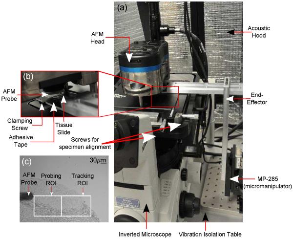
The experimental setup consists of the Atomic Force Microscope (MFP-3D-BIO™, Asylum Research) and an inverted microscope (Model: TE2000U, Nikon, Inc) with an attached CCD camera (QImaging Inc, Model: Retiga 2000R). At the base of the microscope is a motorized micromanipulator MP-285 (Sutter Instruments, Inc), to which is attached an end-effector used to hold the microscope slide. The AFM, inverted microscope and the micromanipulator are placed on a vibration isolation table to eliminate base vibrations [Fig. 1(a,b)].

Fig. 1.

(a) and (b) AFM Experimental Setup with the MP-285 micromanipulator, (c) brightfield image of AFM indentation process.

We used closed-loop image-guided positioning to align the tissue specimens and the AFM probe tip. Briefly, a region-of-interest (ROI) corresponding to one of the annotated regions was selected by the user (called the “Probing ROI”), and an adjacent ROI (called the “Tracking ROI”) was used to provide image feedback [Fig. 1(c)]. A gradient-descent based controller was used to precisely position the probing point underneath the probe tip within 1μm. Following accurate positioning, indentations were performed on the “Probing ROI” in a raster fashion. Please refer to [29] for further details on the experimental setup.

C. AFM Probe Spring Constant Calibration

We used the thermal method to calibrate the AFM probe spring constant in our experiments [14]. The thermal method is particularly attractive compared to the Sader method because this method does not require exact knowledge of the dimensions of the probe [16]. In this calibration scheme, the probe is assumed to behave as a simple harmonic oscillator (SHO), vibrating in response to thermal noise in its vicinity. Using the equipartition theorem, we get [14]:

$$\frac{1}{2}m{\omega }_0^2\langle p^2\rangle =\frac{1}{2}{k}_{B}T$$

or

$$k_c\langle p^2\rangle =k_{B}T$$ (1)

where k_c is the probe spring constant (N/m), m is the equivalent mass of the AFM probe (kg), T is the ambient temperature (K), k_B is the Boltzmann constant (J/K), ⟨p²⟩ is the mean of the square of the probe deflection, p (m), and ω₀ (Hz) is the fundamental frequency of the probe. When analyzed in the frequency domain, the spring constant is represented as:

$$k_c=\frac{k_{B}T}{P}$$ (2)

where P is the integral of the Power Spectral Density (PSD), which equals the mean square of the probe deflections.

Since the probe deflection is optically measured through the photodiode, the calibration experiment includes estimation of a conversion term, commercially termed as Inverse Optical Lever Sensitivity (InvOLS), which also includes a correction factor that account for the approximation of AFM probes as ideal springs [30] and the finite laser spot at the probe end [31]. The InvOLS is estimated by taking an AFM force curve on a hard surface, typically a tissue-free location on the microscope slide. The final calibrated spring constant is given by:

$$k_c=\frac{k_{B}T}{P{\left(\mathit{InvOLS}\right)}^2}$$ (3)

It is worth mentioning here that henceforth we use the probe compliance, s = 1/k_c, instead of the spring constant. This transformation allows us to integrate the variability observed in the calibration results into the EIV model, as shown later in Section III.

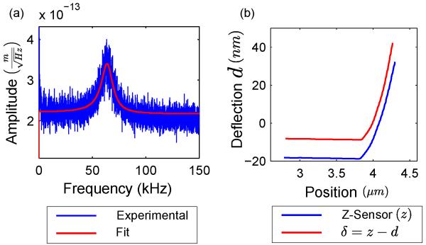
Representative results of 20 calibration experiments for two probes in PBS solution prior to and after the completion of the AFM experiment are displayed in Table I. As seen in Fig. 2(a) (PSD of the probe with nominal compliance = 0.222 m/N), the location of the fundamental frequency is not sharp, due to low Q-factor in liquid. As a result, fitting the PSD to a Lorentzian function to compute P is prone to errors and could be one of the contributing factors behind the variability in the probe’s fundamental frequency shown in Table I. The overall variability of the calibrated probe compliance is ~ 10%, which is in good agreement with previously reported uncertainty with the thermal calibration method [15]. In this work, we use the second probe (probe with nominal compliance = 0.222 m/N) for the indentation experiments and subsequent data analysis.

TABLE I.

AFM probe calibration results

Nominal Probe Compliance (m/N)	InvOLS† (nm/V)	Fundamental Freq.†(kHz)	Calibrated Probe Compliance†(m/N)
16.667	87.72 ± 3.66	3.774 ± 0.125	16.382 ± 1.634
0.222	178.36 ± 1.88	62.675 ± 2.745	0.328 ± 0.032

^†Results shown as mean ± standard deviation.

Fig. 2.

(a) Thermal spectrum of the probe oscillating in PBS, with overlaid Lorentzian fit in red. (b) Representative AFM force curve on breast tissue. Note that the d vs. δ curve is displaced 10 nm on the deflection axis for ease of visualization.

III. BAYESIAN ANALYSIS

A. Force-Indentation relationship

The extraction of material parameters typically requires fitting an appropriate contact model to the experimental AFM data. A widely used analytical formulation for this purpose is the Hertz contact model [32]. Fundamental assumptions in Hertzian contact theory are that the sample indented is a homogeneous, isotropic elastic half-space subject to infinitesimal strains. Additional assumptions include adhesion-free frictionless contact and linear elasticity in the material.

However, in our studies, many of these assumptions do not apply. The breast tissue specimens we studied were highly heterogeneous - the sampled tissue includes functional breast epithelial cells that are enclosed by collagen-rich stromal tissue [29]. Moreover, most biological specimens, particularly tissue samples, exhibit nonlinear constitutive behavior [33]. Furthermore, the tissue specimens are of finite thickness (~ 4μm) compared to the depth of indentation (~ 100 - 600 nm) and the geometry of the spherical particle attached to the AFM probe (radius = 2.5μm), which invalidates the assumptions of infinitesimal strains in Hertzian contact theory.

As a result, we use a contact model developed by Long et al [28] which accounts for geometric and material nonlinearities during spherical indentation. The contact force, F, is related to the indentation, Δ, in an incompressible neo-Hookean material by:

$$\begin{array}{cc}\hfill F=& \frac{16E\sqrt{R}}{9}[{\Delta }^{1.5}+1.15\sqrt{\gamma }{\Delta }^2+{\alpha }_1\gamma \sqrt{\gamma }{\Delta }^3\phantom{]}\hfill \\ \hfill & +\phantom{[}{\alpha }_2{\gamma }^3{\Delta }^{4.5}]/\left[1+2.3\gamma \sqrt{\gamma }{\Delta }^{1.5}\right]\hfill \end{array}$$ (4)

where

$${\alpha }_1=10.05-0.63\sqrt{h∕R}(3.10+h^2∕R^2)$$ (5a)

$${\alpha }_2=4.8-4.23h^2∕R^2$$ (5b)

$$\gamma =R∕h^2$$ (5c)

E is the elastic modulus, R is the radius of the spherical bead and h is the thickness of the tissue sample. Long’s force-indentation relationship is valid in the regime Δ/h ≤ min(0.6, R/h) and 0.3 ≤ R/h ≤ 12.7 [28]. The expressions in Eqns. 5(a) and 5(b) assume frictionless contact, which is a reasonable assumption since the tissue specimens are hydrated in PBS solution during the AFM experiments.

B. Transformation of raw data

The AFM probe deflection (d) and z-position (z) values are processed offline to estimate the elastic properties of the specimen being studied. A typical AFM curve is shown in Fig. 2(b). Given n data points, the tip touches the sample at position (z_k, d_k), where k ∈ (1, n) is the unknown index in the dataset which indicates the transition from non-contact to the contact regime.

In the contact regime, the net indentation in the sample is given by Δ = (z_n − z_k) − (d_n − d_k) = δ_n − δ_k [34], using the relation: δ_i = z_i − d_i. Assuming that the probe behaves as a linear spring for low deflection ranges, the force of indentation is given as F = k_cd where k_c is the probe spring constant. Using the probe compliance, s = 1/k_c, instead of the probe spring constant, and the contact model described in section III.A, Eqn. 4 can be written as:

$$d_i-d_k=\frac{16E\sqrt{R}}{9}{\mathit{sf}}_i$$ (6)

where

$$\begin{array}{cc}\hfill f_i=& [{({\delta }_i-{\delta }_k)}^{1.5}+1.15\sqrt{\gamma }{({\delta }_i-{\delta }_k)}^2+{\alpha }_1\gamma \sqrt{\gamma }{({\delta }_i-{\delta }_k)}^3\phantom{]}\hfill \\ \hfill & +\phantom{[}{\alpha }_2{\gamma }^3{({\delta }_i-{\delta }_k)}^{4.5}]/\left[1+2.3\gamma \sqrt{\gamma }{({\delta }_i-{\delta }_k)}^{1.5}\right]\hfill \end{array}$$ (7)

where k + 1 ≤ i ≤ n and Δ is replaced by the transformed variable δ.

Using the probe compliance, s, in Eqn. 6 allows us to relate the deflection, d, to the transformed variable δ, and to incorporate the probe compliance into the EIV model, as shown later in Section III.C.

In the non-contact regime, the deflection can be modeled as a linear function of z [35], i.e. d = az + b. Using the transformed variable, δ, we may rewrite the non-contact region as d = aδ/(1−a)+b/(1−a), thus preserving the linear nature of the non-contact regime.

Therefore, the two-regime regression model can be written as:

$$d_i=\{\begin{array}{cc}\left[1{\delta }_i\right]{\beta }_1+{∊}_1\hfill & \text{if}i\le k\hfill \\ \left[1{\mathit{sf}}_i\right]{\beta }_2+{∊}_2\hfill & \text{if}k+1\le i\le n\hfill \end{array}\phantom{\}}$$ (8)

where ∊_j ~ N(0, σ_j²)j = 1, 2. are independent and identically distributed (i.i.d) normal random variables and f_i is given by Eqn. 7. In general, ${\sigma }_1^2\ne {\sigma }_2^2$, since ${\sigma }_1^2$ results from the viscous interactions between the probe and the PBS solution, while ${\sigma }_2^2$ depends primarily on the probe-tissue frictional forces [22]. ${\beta }_j={\left[\begin{array}{cc}\hfill {\beta }_{j1}\hfill & \hfill {\beta }_{j2}\hfill \end{array}\right]}^T$ ; j = 1, 2 are the regression coefficients in the non-contact and contact regime respectively.

C. EIV-based Bayesian Changepoint Model

1) Classical EIV Model

We use the notation as given in [26] to represent the EIV model. In the linear EIV model in classical form, the unobservable variables ξ and η are related by [26]:

$${\eta }_i={\beta }_0+{\beta }_1{\xi }_{i}i=1,2,\dots ,n.$$ (9)

Instead of observing (ξ_i, η_i), the pair (x_i, y_i), i = 1, 2, …, n is observed with errors (ν_i, ∊_i), which are assumed normal. The response variable y_i’s are given by:

$$y_i={\eta }_i+{∊}_i$$ (10)

The observed covariates x_i’s are given by:

$$x_i={\xi }_i+{\nu }_i$$ (11)

We use ν instead of δ to specify the errors in Eqn. 11 as used in [26], to maintain conformity with the previously described transformed variable δ. We use standard (i.i.d) assumptions [26]:

$$E\left({\nu }_i\right)=E\left({∊}_i\right)=0\forall i$$ (12a)

$$\mathit{var}\left({\nu }_i\right)={\sigma }_{\nu }^2,\mathit{var}\left({∊}_i\right)={\sigma }_{∊}^2\forall i$$ (12b)

$$\mathit{cov}({\nu }_i,{\nu }_j)=\mathit{cov}({∊}_i,{∊}_j)=0\forall i\ne j$$ (12c)

$$\mathit{cov}({\nu }_i,{∊}_j)=0\forall i,j.$$ (12d)

The data likelihood is given as the joint distribution of the pair (x_i, y_i), i = 1, 2, …, n, and is stated as follows [26]:

$$\begin{array}{cc}\hfill & p(x_1,\dots ,x_n,y_1,\dots ,y_n\mid {\beta }_0,{\beta }_1,{\sigma }_{\nu }^2,{\sigma }_{∊}^2,{\xi }_i,\dots ,{\xi }_n)\hfill \\ \hfill & \propto \prod _{i=1}^n{\left[\frac{1}{{\sigma }_{\nu }^2}\right]}^{\frac{1}{2}}{e}^{\left[-\frac{1}{2{\sigma }_{\nu }^2}{(x_i-{\xi }_i)}^2\right]}\times \prod _{i=1}^n{\left[\frac{1}{{\sigma }_{∊}^2}\right]}^{\frac{1}{2}}{e}^{\left[-\frac{1}{2{\sigma }_{∊}^2}{(y_i-{\beta }_0-{\beta }_1{\xi }_i)}^2\right]}\hfill \end{array}$$ (13)

2) EIV-based Changepoint Modeling

In the non-contact regime (Eqn. 8, i ≤ k), the covariates ξ’s are given by ξ_i = δ_i, i = 1, 2, …, k, which are fixed and observed. In the contact regime (Eqn. 8, k + 1 ≤ i ≤ n), we can write:

$$\begin{array}{cc}\hfill & {\xi }_{k+1}={\mathit{sf}}_{k+1}\hfill \\ \hfill & ⋮\hfill \\ \hfill & {\xi }_n={\mathit{sf}}_n\hfill \end{array}$$ (14)

The covariates ξ_k+1, …, ξ_n in Eqn. 14 are multiples of the probe compliance s. When s is observed without errors, the estimation approach proposed in this work reduces to the regular Bayesian Changepoint model [22],[36], since ξ₁, …, ξ_n are fixed and observed. However, variations in the probe calibration results as evidenced by the results in Table I indicate that incorporation of some notion of randomness on the nature of s is necessary.

We model s as an unobserved variable which needs to be estimated. Instead of observing s, we observe s_d with an additive Gaussian error $\psi \sim N(0,{\sigma }_{s_d}^2)$, which is given by:

$$s_d=s+\psi ;\psi \sim N(0,{\sigma }_{s_d}^2)$$ (15)

Using the observed probe compliance s_d, we can write:

$$\begin{array}{cc}\hfill & x_{k+1}=s_d{f}_{k+1}\hfill \\ \hfill & ⋮\hfill \\ \hfill & x_n=s_d{f}_n\hfill \end{array}$$ (16)

where x_k+1, …, x_n are the observed covariates analogous to the observed x_i’s in Eqn. 11.

At this point, it would seem natural to define a joint distribution of the data (x_i, d_i) similar to Eqn. 13. However, from Eqn. 16, it is clear that x_k+1, …, x_n are not independent; instead, they are multiples of s_d. Moreover, it is important to note that the independence condition from Eqn. 12(c) is violated, since:

$$\begin{array}{cc}\hfill \mathit{cov}({\nu }_i,{\nu }_j)& =\mathit{cov}(x_i,x_j)=f_i{f}_j\mathit{cov}(s_d,s_d)\hfill \\ \hfill & \ne 0\forall i\ne j\hfill \end{array}$$ (17)

As a result, the covariate distribution can simply be expressed in s_d and s, instead of the covariates x_k+1, …, x_n and ξ_k+1, …, ξ_n respectively. The EIV model in the contact regime therefore reduces to the scalar equation represented by Eqn. 15.

3) Data Likelihood and Posterior

The two regime regression model from Eqn. 8 can be compactly written as:

$$d_i\mid s\sim \{\begin{array}{cc}N({\beta }_{11}+{\beta }_{12}{\delta }_i,{\sigma }_1^2)\hfill & \text{if}i\le k\hfill \\ N({\beta }_{21}+s{\beta }_{22}{f}_i,{\sigma }_2^2)\hfill & \text{if}k+1\le i\le n\hfill \end{array}\phantom{\}}$$ (18)

Based on the preceding discussion, the data likelihood can be expressed using the pair (s_d, d), and is given as:

$$\begin{gathered} p(s_d,d_1,d_2,\dots ,d_n\mid {\beta }_1,{\beta }_2,{\sigma }_1^2,{\sigma }_2^2,k,s) \\ \propto {\left[\frac{1}{{\sigma }_{s_d}^2}\right]}^{\frac{1}{2}}{e}^{\left[\frac{-{(s_d-s)}^2}{2{\sigma }_{s_d}^2}\right]}\times \prod _{i=1}^k{\left[\frac{1}{{\sigma }_1^2}\right]}^{\frac{1}{2}}{e}^{\left[-\frac{1}{2{\sigma }_1^2}{(d_i-{\beta }_{11}-{\beta }_{12}{\delta }_i)}^2\right]} \\ \times \prod _{i=k+1}^n{\left[\frac{1}{{\sigma }_2^2}\right]}^{\frac{1}{2}}{e}^{\left[-\frac{1}{2{\sigma }_2^2}{\{d_i-{\beta }_{21}-s{\beta }_{22}{f}_i\}}^2\right]} \end{gathered}$$ (19)

For a given candidate contact point k, we can rewrite the deflection data in a compact vector form, as, ${\mathit{d}}_1^k={\left[\begin{array}{cccc}\hfill d_1\hfill & \hfill d_2\hfill & \hfill \dots \hfill & \hfill d_k\hfill \end{array}\right]}^T$ and ${\mathit{d}}_2^k={\left[\begin{array}{cccc}\hfill d_{k+1}\hfill & \hfill d_{k+2}\hfill & \hfill \dots \hfill & \hfill d_n\hfill \end{array}\right]}^T$ and $\mathbf{d}={\left[\begin{array}{cc}\hfill {\mathbf{d}}_1^k\hfill & \hfill {\mathbf{d}}_2^k\hfill \end{array}\right]}^T$. The right hand side of Eqn. 8 can be written as:

$$\begin{array}{c}\hfill {\mathit{X}}_1^k={\left[\begin{array}{cccc}\hfill 1\hfill & \hfill 1\hfill & \hfill \dots \hfill & \hfill 1\hfill \\ \hfill {\delta }_1\hfill & \hfill {\delta }_2\hfill & \hfill \dots \hfill & \hfill {\delta }_k\hfill \end{array}\right]}^T\hfill \\ \hfill {\mathit{X}}_2^k={\left[\begin{array}{cccc}\hfill 1\hfill & \hfill 1\hfill & \hfill \dots \hfill & \hfill 1\hfill \\ \hfill {\mathit{sf}}_{k+1}\hfill & \hfill {\mathit{sf}}_{k+2}\hfill & \hfill \dots \hfill & \hfill {\mathit{sf}}_n\hfill \end{array}\right]}^T\hfill \end{array}$$ (20)

Using the notations in Eqn. 20, the data likelihood can be re-written as:

$$\begin{array}{cc}\hfill p(s_d,\mathit{d}\mid {\beta }_1,{\beta }_2,{\sigma }_1^2,{\sigma }_2^2,k,s)\propto & {\left[\frac{1}{{\sigma }_{s_d}^2}\right]}^{\frac{1}{2}}{e}^{\left[-\frac{1}{2{\sigma }_{s_d}^2}{(s_d-s)}^2\right]}\times \hfill \\ \hfill {\left[\frac{1}{{\sigma }_1^2}\right]}^{\frac{k}{2}}{e}^{\left[-\frac{1}{2{\sigma }_1^2}{\Vert {\mathit{d}}_1-{\mathit{X}}_1{\beta }_1\Vert }^2\right]}\times & {\left[\frac{1}{{\sigma }_2^2}\right]}^{\frac{n-k}{2}}{e}^{\left[-\frac{1}{2{\sigma }_2^2}{\Vert {\mathit{d}}_2-{\mathit{X}}_2{\beta }_2\Vert }^2\right]}\hfill \end{array}$$ (21)

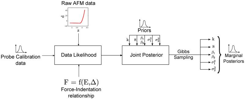
We use conjugate priors (Table II) to ensure that the posterior distribution is separable (please refer to Fig. 3 for schematic) [36]. The posterior distribution, expressed as posterior distribution ∝ data likelihood × prior distribution, can be written as:

$$\begin{array}{cc}\hfill & p({\beta }_1,{\beta }_2,{\sigma }_1^2,{\sigma }_2^2,k,s\mid s_d,\mathit{d})\propto p(\mathit{d},s_d\mid {\beta }_1,{\beta }_2,{\sigma }_1^2,{\sigma }_2^2,k,s)\hfill \\ \hfill & \times \pi \left({\beta }_1\right)\times \pi \left({\beta }_2\right)\times \pi \left({\sigma }_1^2\right)\times \pi \left({\sigma }_2^2\right)\times \left(k\right)\times \pi \left(s\right)\hfill \end{array}$$ (22)

where π(.) indicates the prior distribution of the variable in parenthesis. Combining the distribution of the data with the priors, we get the posterior as:

$$\begin{array}{cc}\hfill & p({\beta }_1,{\beta }_2,{\sigma }_1^2,{\sigma }_2^2,k,s\mid s_d,\mathit{d})\propto {\left[\frac{1}{{\sigma }_1^2}\right]}^{\frac{k}{2}}{\left[\frac{1}{{\sigma }_2^2}\right]}^{\frac{n-k}{2}}{\left[\frac{1}{{\sigma }_{s_d}^2}\right]}^{\frac{1}{2}}\hfill \\ \hfill & \times e^{\left[-\frac{1}{2{\sigma }_1^2}{\Vert {\mathit{d}}_1-{\mathit{X}}_1{\beta }_1\Vert }^2\right]}{e}^{\left[-\frac{1}{2{\sigma }_2^2}{\Vert {\mathit{d}}_2-{\mathit{X}}_2{\beta }_2\Vert }^2\right]}{e}^{\left[-\frac{1}{2{\sigma }_{s_d}^2}{(s_d-s)}^2\right]}\hfill \\ \hfill & \times e^{\left[-\frac{1}{2}{({\beta }_1-{\stackrel{‒}{\beta }}_1)}^T{\stackrel{‒}{\Lambda }}_1({\beta }_1-{\stackrel{‒}{\beta }}_1)\right]}{e}^{\left[-\frac{1}{2}{({\beta }_2-{\stackrel{‒}{\beta }}_2)}^T{\stackrel{‒}{\Lambda }}_2({\beta }_2-{\stackrel{‒}{\beta }}_2)\right]}\hfill \\ \hfill & \times {\left({\sigma }_1^2\right)}^{-a_0-1}{e}^{\left[-\frac{b_0}{{\sigma }_1^2}\right]}{\left({\sigma }_2^2\right)}^{-a_0-1}{e}^{\left[-\frac{b_0}{{\sigma }_2^2}\right]}{\left[\frac{1}{{\sigma }_{s_p}^2}\right]}^{\frac{1}{2}}{e}^{\left[-\frac{1}{2{\sigma }_{s_p}^2}{(s-{\mu }_{s_p})}^2\right]}\hfill \end{array}$$ (23)

TABLE II.

Conjugate Prior Distributions

Model Parameter	Distribution Family	Hyperparameters
k	Uniform	~ U (1, n)
β1, β2	Normal	$~N({\stackrel{‒}{\beta }}_1,{\stackrel{‒}{\Lambda }}_1^{-1}),~N({\stackrel{‒}{\beta }}_2,{\stackrel{‒}{\Lambda }}_2^{-1})$
${\sigma }_1^2,{\sigma }_2^2$	Inverse Gamma	~ IG(a0 ,b0) , ~ IG(a0 ,b0)
s	Normal	$~N({\mu }_{s_p},{\sigma }_{s_p}^2)$

Fig. 3.

Schematic of the EIV-Bayesian Changepoint algorithm.

4) Gibbs Sampling

The marginal posterior distribution for each parameter in Eqn. 23 is obtained using Gibbs Sampling [37]. Each marginal posterior is derived by separating out the terms in the posterior distribution of Eqn. 23 corresponding to the given parameter and conditional on the rest. After some algebraic manipulations [38], we get the following sampled parameters for each step i of the Gibbs Sampler:

$$\begin{array}{cc}\hfill s^{(i+1)}& \sim p(s\mid {\beta }_1^{\left(i\right)},{\beta }_2^{\left(i\right)},{\sigma }_1^{2,\left(i\right)},{\sigma }_2^{2,\left(i\right)},k^{\left(i\right)})\hfill \\ \hfill & =N({\tilde{\mu }}_s,{\tilde{\sigma }}_s^2)\hfill \end{array}$$ (24a)

$$\begin{array}{cc}\hfill {\beta }_1^{(i+1)}& \sim p({\beta }_1\mid s^{(i+1)},{\beta }_2^{\left(i\right)},{\sigma }_1^{2,\left(i\right)},{\sigma }_2^{2,\left(i\right)},k^{\left(i\right)})\hfill \\ \hfill & =N({\tilde{\beta }}_1,{\tilde{\Sigma }}_1)\hfill \end{array}$$ (24b)

$$\begin{array}{cc}\hfill {\beta }_2^{(i+1)}& \sim p({\beta }_2\mid s^{(i+1)},{\beta }_1^{(i+1)},{\sigma }_1^{2,\left(i\right)},{\sigma }_2^{2,\left(i\right)},k^{\left(i\right)})\hfill \\ \hfill & =N({\tilde{\beta }}_2,{\tilde{\Sigma }}_2)\hfill \end{array}$$ (24c)

$$\begin{array}{cc}\hfill {\sigma }_1^{2,(i+1)}& \sim p({\sigma }_1^2\mid s^{(i+1)},{\beta }_1^{(i+1)},{\beta }_2^{(i+1)},{\sigma }_2^{2,\left(i\right)},k^{\left(i\right)})\hfill \\ \hfill & =\mathit{IG}({\tilde{a}}_1,{\tilde{b}}_1)\hfill \end{array}$$ (24d)

$$\begin{array}{cc}\hfill {\sigma }_2^{2,(i+1)}& \sim p({\sigma }_2^2\mid s^{(i+1)},{\beta }_1^{(i+1)},{\beta }_2^{(i+1)},{\sigma }_1^{2,(i+1)},k^{\left(i\right)})\hfill \\ \hfill & =\mathit{IG}({\tilde{a}}_2,{\tilde{b}}_2)\hfill \end{array}$$ (24e)

$$k^{(i+1)}\sim p(k\mid s^{(i+1)},{\beta }_1^{(i+1)},{\beta }_2^{(i+1)},{\sigma }_1^{2,(i+1)},{\sigma }_2^{2,(i+1)})$$ (24f)

where the parameters of the marginal posterior densities are:

$${\tilde{\mu }}_s=[\left(\frac{{\sigma }_{s_p}^2{s}_d+{\sigma }_{s_d}^2{\mu }_{s_p}}{{\sigma }_{s_p}^2+{\sigma }_{s_d}^2}\right)\frac{{\sigma }_2^2}{{\beta }_{22}^2\sum _{j=k+1}^n{f}_j^2}\phantom{]}+\phantom{[}\left(\frac{\sum _{j=k+1}^n(d_j-{\beta }_{21})f_j}{{\beta }_{22}\sum _{j=k+1}^n{f}_j^2}\right)\left(\frac{{\sigma }_{s_p}^2{\sigma }_{s_d}^2}{{\sigma }_{s_p}^2+{\sigma }_{s_d}^2}\right)]{\left[\frac{{\sigma }_2^2}{{\beta }_{22}^2\sum _{j=k+1}^n{f}_j^2}+\left(\frac{{\sigma }_{s_p}^2{\sigma }_{s_d}^2}{{\sigma }_{s_p}^2+{\sigma }_{s_d}^2}\right)\right]}^{-1}$$ (25a)

$${\tilde{\sigma }}_s^2={\left[\frac{{\beta }_{22}^2}{{\sigma }_2^2}\sum _{j=k+1}^n{f}_j^2+\frac{1}{{\sigma }_{s_d}^2}+\frac{1}{{\sigma }_{s_p}^2}\right]}^{-1}$$ (25b)

$$\begin{array}{cc}\hfill {\tilde{\beta }}_m=& {({\sigma }_m^{-2}{{\mathit{X}}_m^{}}^T{\mathit{X}}_m^k+{\stackrel{‒}{\Lambda }}_m)}^{-1}({\sigma }_m^{-2}{{\mathit{X}}_m^k}^T{\mathit{d}}_m^k\hfill \\ \hfill & +{\stackrel{‒}{\Lambda }}_m{\stackrel{‒}{\beta }}_m)\hfill \end{array}$$ (25c)

$${\tilde{\Sigma }}_m={({\sigma }_m^{-2}{{\mathit{X}}_m^k}^T{\mathit{X}}_m^k+{\stackrel{‒}{\Lambda }}_m)}^{-1}$$ (25d)

$${\tilde{a}}_1=a_0+k∕2$$ (25e)

$${\tilde{a}}_2=a_0+(n-k)∕2$$ (25f)

$${\tilde{b}}_m=b_0+0.5{(\Vert {\mathit{d}}_m^k-{\mathit{X}}_m^k{\beta }_m\Vert )}^2$$ (25g)

where m = 1, 2 for the non-contact and the contact regimes respectively.

IV. RESULTS

A. Implementation of the Gibbs Sampler

Excepting the contact point index k, all the other marginal posteriors can be directly sampled from their respective family of parametric probability distributions due to the use of conjugate priors. We used rejection sampling [39] to sample for k [Eqn. 24(f)] to complete the Gibbs Sampling step.

We reject the initial 3000 iteration results of the Gibbs Sampler which constitutes the burn-in period. Sampling is terminated when increasing the number of iterations do not alter the nature of the marginal distributions. Typically, we sample for 200,000 iterations. With respect to the probe compliance, we set s_d to a pre-experiment calibration value (= 0.339 m/N). We set the hyperparameter values of the probe compliance to those obtained in Table I, i.e. μ_sp = 0.328 m/N, ${\sigma }_{s_p}^2={0.032}^2{m}^2∕N^2$. Using such an informative prior based on Table I allows us to incorporate prior knowledge of multiple probe calibrations. We also assume that the prior and data variances of the probe compliance are the same i.e. ${\sigma }_{s_p}^2={\sigma }_{s_d}^2$. This allows us to give equal weightage to the prior and data values. With respect to the other parameters, no useful information is available beforehand, consequently, uninformative priors are assigned to them. The contact point k is assigned a uniform distribution, U(1, n), while, β₁, β₂, ${\sigma }_1^2$ and ${\sigma }_2^2$ are assigned dispersed prior distributions. The hyperparameter values used during sampling are given in Table III.

TABLE III.

Hyperparameter Values

Hyperparameters	Values
${\stackrel{‒}{\beta }}_1,{\stackrel{‒}{\beta }}_2$	${\left[\begin{array}{cc}\hfill 0\hfill & \hfill 0\hfill \end{array}\right]}^T$
${\stackrel{‒}{\Lambda }}_1,{\stackrel{‒}{\Lambda }}_2$	$\left[\begin{array}{cc}\hfill {10}^{-15}\hfill & \hfill 0\hfill \\ \hfill 0\hfill & \hfill {10}^{-15}\hfill \end{array}\right]$
(a0, b0)	(1, 0.002)
$({\mu }_{s_p},{\sigma }_{s_p}^2)$	(0.328, 0.0322)

B. AFM Indentation Studies

During AFM experiments, the probe deflection was fixed at 50 nm, leading to approximately 100 - 600 nm indentations in the sample. The loading velocity was kept constant at 1.98μm/sec.

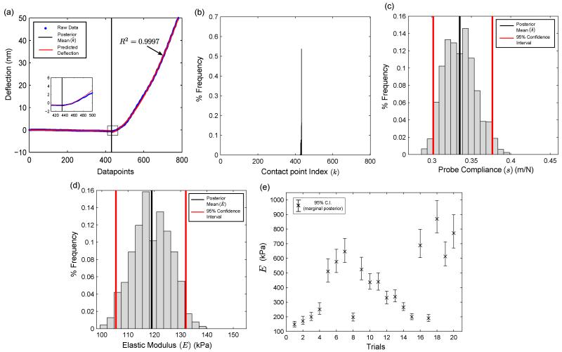
Fig. 4 summarizes the results of our EIV-Changepoint analysis applied on AFM indentation data on tissue specimens. The AFM deflection data with the posterior mean of the contact point ($\widehat{k}=433$), and the marginal posterior distribution of k are shown in Fig. 4(a) and 4(b) respectively. It is evident from Fig. 4(a) that Long’s contact model appropriately describes the force curve shown in this figure (R² = 0.9997).

Fig. 4.

Results of Gibbs Sampling on the posterior distribution. (a) Representative AFM deflection curve on a tissue sample (n = 781) data points, (b) marginal posterior in the contact point k, (c) marginal posterior of the probe compliance s, (d) marginal posterior of elastic modulus E (linearly related to β₂₂), and (e) mean and 95% confidence intervals on multiple datasets. Note: Only those force curves with R² > 0.99 have been shown in Fig. 4(e).

The marginal posterior in s is shown in Fig. 4(c). The marginal posterior in β₂₂ [Fig. 4(d)] is easily transformed into the elastic modulus, E, due to the linear relationship between them (Eqn. 6). The posterior mean of the elastic modulus is computed to be $\widehat{E}=119.01\mathrm{kPa}$. Across 20 datasets [Fig. 4(e)], the elastic modulus is found to vary between 100-1000 kPa, which compares favorably with our previously reported values on human breast tissue [29].

It is should be noted here that in Fig. 4, we have implemented our algorithm only on those AFM datasets which had a good fit (with overall R² > 0.99) with Long’s contact model. As observed previously in [40], biological tissue samples are spatially heterogeneous specimens, not only in the magnitude of its elastic modulus as shown in Fig. 4(e), but also the type of constitutive material model that accurately describes it. Indeed, there were populations of AFM force curves that did not follow neo-Hookean material behavior and we have not included those datasets in this work. At this point of our research, we are not looking to establish the most appropriate contact model for any given AFM force curve, and we intend to investigate this in the future.

C. Sensitivity Tests

The dispersed nature of the marginal posterior in E of Fig. 4(d) raises an interesting question - what are the individual contributions of the contact point uncertainty and the probe compliance variability to the marginal posterior distribution in E ? More importantly, does the marginal posterior in E reflect changes in the hyperparameter values of the probe compliance, given that an informative prior was used for it?

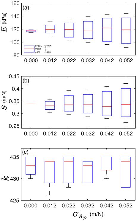
In Fig. 5, we illustrate the effect of using hypothetical values of σ_sp in the posterior distribution. The dispersion in the marginal posterior in E increases with σ_sp, as shown in Fig. 5(a). This is expected, since larger variations in the calibrated probe compliance would lead to greater uncertainty in the elastic modulus of the probed regions. The individual contribution of contact point uncertainty on the marginal posterior in E is given in the first boxplot of Fig. 5(a) (corresponding to σ_sp = 0.000).

Fig. 5.

Boxplots indicating the effect of varying σ_sp on the marginal posteriors (a) in E, (b) in s and (c) in k, Please note that the σ_sd has been assumed to be equal to σ_sp. The fourth boxplot (σ_sp = 0.032 m/N) corresponds to the experimental probe compliance variance as obtained in Table I.

Likewise, increase in σ_sp leads to greater dispersion in the marginal posteriors in s [Fig. 5(b)]. It is worth noting that changes in σ_sp does not cause any substantial change to the posterior means of E or s.

The boxplots of Fig. 5(c) shows the effect of σ_sp on the marginal posterior in k. Changes in σ_sp has no significant effect on the posterior in k: the 95% confidence interval of k ranges between the 428^th and 435^th datapoints for all the boxplots. This is an important observation, since uncertainties in the probe compliance and the contact point are physically unrelated - probe compliance variations are the result of calibration errors, while contact point uncertainty occurs because of the soft nature of biological tissues and the absence of a perceptible attractive region in the AFM force curve in liquid.

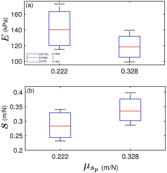
Next, we show the effect of varying the hyperparameter μ_sp on the marginal posteriors in E [Fig. 6(a)] and s [Fig. 6(b)]. We retain the previous values of s_d(= 0.339) m/N and σ_sd (= 0.032) m/N and the assumption that ${\sigma }_{s_d}^2={\sigma }_{s_p}^2$. The first boxplot shows the marginal posteriors when μ_sp is set to 0.222 m/N, the probe manufacturer’s nominal compliance. This is often useful when the AFM user performs a single probe calibration experiment, and wishes to see the result of using the nominal compliance instead of repeating the calibration experiments. The second boxplot uses μ_sp = 0.328 m/N, obtained from Table I.

Fig. 6.

Boxplots indicating the effect of varying μ_sp on the marginal posteriors (a) in E and (b) in s. The first boxplot with μ_sp = 0.222 m/N corresponds to the case where the probe manufacturer’s nominal compliance is used as the hyperparameter.

Reducing the hyperparameter μ_sp from 0.328 m/N to 0.222 m/N leads to an increasing trend in the marginal posterior in E [Fig. 6(a)] and a corresponding decreasing trend in the marginal posterior in s [Fig. 6(b)]. This is understandable, given the inverse relationship between s and E (see Eqn. 6). This inverse relationship is also responsible for the increased dispersion in the first boxplot of Fig. 6(a) compared to the second; in contrast, both boxplots in Fig. 6(b) show largely similar dispersed behavior.

It is also evident from Fig. 6(b) that the probe compliance posterior means (ŝ) lie approximately midway between the compliance data s_d and the hyperparameter μ_sp (ŝ = 0.283 m/N for μ_sp = 0.222 m/N and ŝ = 0.333 m/N for μ_sp = 0.328 m/N). This is a direct consequence of using equal weightage to the data and prior variances of the probe compliance, i.e. (${\sigma }_{s_d}^2={\sigma }_{s_p}^2$).

V. DISCUSSION

In this work, we have presented an integrated probabilistic approach to quantify the elastic properties of biomaterials undergoing AFM indentation after accounting for contact point uncertainty and AFM probe spring constant variations. Using a EIV-Bayesian Changepoint framework, we have generated posterior distributions of the contact point and the elastic modulus of regions in breast tissue specimens that follow a neo-Hookean hyperelastic relationship. A sensitivity analysis on the parameters of the posterior distribution showed that our model responded satisfactorily to a wide range of hyperparameter values.

It is also worthwhile noting that our algorithm is independent of the choice of the contact model, so long as the force-indentation relationship is linear in the elastic modulus E. Indeed, setting γ = 0 (for the case h → ∞) reduces Eqn. 4 to the Hertz contact model [32].

Another appealing aspect of our approach is that it makes it possible to automate data analysis of AFM force curves. Typically, AFM indentation studies on tissue specimens for histopathological inference necessitates very large scale AFM indentation data acquisition and processing. A robust and computationally efficient approach can significantly improve throughput of AFM based characterization of biomaterials.

We would like to emphasize that the purpose of this study is not to develop constitutive material models for soft biological specimens undergoing AFM indentation, rather to develop a fairly detailed statistical framework to quantify uncertainties occuring in AFM indentation experiments on soft biomaterials. As mentioned previously in Section IV.B, a single contact model does not adequately describe all force curves acquired from raster indentation experiments on tissue samples due to the underlying material heterogeneity in the specimens. One possible estimation approach that could account for material heterogeneity in tissue specimens is to use inverse finite-element based methods that utilize various hyperelastic constitutive laws to model the post-contact AFM force curve. The contact point and the material properties can then be estimated reliably after a suitable hyperelastic model has been selected to describe the force curve in question.

Another possible extension of our work is to investigate the use of interval uncertainty-integrated hypothesis testing methods [21] for inference studies.

Biographies

Rajarshi Roy (S’11) received the Bachelor of Engineering degree in Mechanical Engineering from Jadavpur University, Kolkata, India in 2008. He is currently a doctoral student in the Robotics, Automation, and Medical Systems (RAMS) Laboratory in the Department of Mechanical Engineering at the University of Maryland, College Park, USA. His research interests include image-guided micromanipulation, AFM based micro-scale tissue characterization and soft tissue biomechanics.

Wenjin Chen received her Bachelor of Medicine degree from Beijing Medical University (now Peking University Medical Center), China and Ph.D. degree from joint program of Molecular Biosciences at University of Medicine and Dentistry of New Jersey and Rutgers University, the State University of New Jersey, 2005. She is currently working as Associate Director of Biomedical Imaging at Center for Biomedical Imaging and Informatics, The Cancer Institute of New Jersey. Her research interests are robotic microscopy, biomedical imaging, quantitative analysis, computer-assisted diagnosis, and medical informatics.

Lei Cong is the Supervisor of Histopathology and Imaging Shared Resources in Cancer Institute of New Jersey (CINJ). She oversees both the Histopathology and IHC Core Services, and the Biospecimen Repository Services (BRS). She has responsibilities for quality control of tissue specimens, tissue microarrays, specimen storage and acquisition, histology and IHC, and biospecimen database managements, etc. She has engaged in many research projects involving tissue microarrays, multispectral imaging analysis, study design, clinical trials, and biomarkers, etc. Lei Cong received her Bachelor of Medicine Degree (MBBS) in China. She has both HTL and QIHC certifications from ASCP.

Lauri Goodell received the Medical degree from University of Medical and Dentistry of New Jersey (UMDNJ) Robert Wood Johnson Medical School, Piscataway, in 1991. She is currently an Associate Professor and the Director of Hematopathology in the Department of Pathology and Laboratory Medicine at UMDNJ Robert Wood Johnson Medical School (RWJMS), as well as the Director of the Immunohistochemistry Core Research Laboratory at The Cancer Institute of New Jersey, New Brunswick. Her current research interests include pathophysiology of hematopoietic diseases, proteomics, image pattern recognition, and telepathology.

David Foran (S’89-M’91) earned a bachelors degree from Rutgers University, New Brunswick, NJ, in 1983 and the Ph.D. degree in biomedical engineering from the University of Medicine and Dentistry of New Jersey (UMDNJ) & Rutgers University, Piscataway, NJ, in 1992. He served as a Physics Instructor at New Jersey Institute of Technology, Newark, NJ, from 1984 to 1985 and worked as a Junior Scientist at Johnson & Johnson Research, Inc., North Brunswick, NJ, from 1986 to 1988. He received one year of post-doctoral training at the Department of Biochemistry at UMDNJ-Robert Wood Johnson Medical School (RWJMS) in 1993. He is currently Professor of Pathology, Laboratory Medicine & Radiology and Chief of the Division of Medical Informatics at Rutgers-Robert Wood Johnson Medical School; and Director of the Center for Biomedical Imaging, Executive Director of Bioinformatics and Chief Medical Informatics Officer at Rutgers Cancer Institute of New Jersey. His research focuses on the design, development, and implementation of new approaches in computer-assisted diagnostics, medical imaging and statistical pattern recognition for resolving challenging clinical problems in pathology, radiology, and oncology. This work has resulted in numerous publications, invited book chapters and several pending and issued patents. Dr. Foran’s research has been funded by the Whitaker Foundation, the NJ Commission on Science & Technology, the federal Defense Advanced Research Projects Agency (DARPA), the Department of Defense (DoD), the Radiological Society of North America, the National Institutes of Health (NIH) and the private sector.

Jaydev P. Desai (S’97-M’97-A’98) is currently a Professor in the Department of Mechanical Engineering at University of Maryland, College Park (UMCP) and the Director of the Robotics, Automation, and Medical Systems (RAMS) Laboratory. He completed his undergraduate studies from the Indian Institute of Technology, Bombay, India, in 1993 with a B.Tech degree. He received his M.A. in Mathematics in 1997, M.S. and Ph.D. in Mechanical Engineering and Applied Mechanics in 1995 and 1998 respectively, all from the University of Pennsylvania. He is a recipient of the NSF CAREER award and the Ralph R. Teetor Educational Award. He was an invited speaker at the 2011 National Academy of Sciences Distinctive Voices at The Beckman Center and was also invited to attend the National Academy of Engineering’s (NAE) 2011 U.S. Frontiers of Engineering Symposium. His research interests include image-guided surgical robotics, haptics, reality-based soft-tissue modeling for surgical simulation, model-based teleoperation in robot-assisted surgery, and micro-scale cell and tissue characterization. He is also a member of the ASME and IEEE.

REFERENCES

- [1].Costa K. Single-cell elastography: Probing for disease with the atomic force microscope. Disease Markers. 2003;19(2-3):139–154. doi: 10.1155/2004/482680. [DOI] [PMC free article] [PubMed] [Google Scholar]
- [2].Suresh S, Spatz J, Mills J, Micoulet A, Dao M, Lim C, Beil M, Seufferlein T. Connections between single-cell biomechanics and human disease states: gastrointestinal cancer and malaria. Acta Biomaterialia. 2005;1:15–30. doi: 10.1016/j.actbio.2004.09.001. [DOI] [PubMed] [Google Scholar]
- [3].Lekka M, Laidler P, Gil D, Lekki J, Stachura Z, Hrynkiewicz AZ. Elasticity of normal and cancerous human bladder cells studied by scanning force microscopy. European Biophyics Journal. 1999;28(4):312–316. doi: 10.1007/s002490050213. [DOI] [PubMed] [Google Scholar]
- [4].Li Q, Lee G, Ong C, Lim C. AFM indentation study of breast cancer cells. Biochemical and Biophysical Research Communications. 2008;374(4):609–613. doi: 10.1016/j.bbrc.2008.07.078. [DOI] [PubMed] [Google Scholar]
- [5].Roy R, Chen W, Goodell L, Hu J, Foran D, Desai J. Microarray-facilitated Mechanical Characterization of Breast Tissue Pathology Samples Using Contact-Mode Atomic Force Microscopy (AFM); IEEE International Conference on Biomedical Robotics and Biomechatronics; 2010.pp. 710–715. [Google Scholar]
- [6].Kim D, Wong P, Park J, Levchenko A, Sun Y. Microengineered Platforms for Cell Mechanobiology. Annual Review of Biomedical Engineering. 2009;11:203–233. doi: 10.1146/annurev-bioeng-061008-124915. [DOI] [PubMed] [Google Scholar]
- [7].Radermacher M. Measuring the elastic properties of living cells by the atomic force microscope. Methods in Cell Biology. 2002;68:67–90. doi: 10.1016/s0091-679x(02)68005-7. [DOI] [PubMed] [Google Scholar]
- [8].Gupta S, Lin J, Ashby P, Pruitt L. A fiber reinforced poroelastic model of nanoindentation of porcine costal cartilage: A combined experimental and finite element approach. Journal of the Mechanical Behavior of Biomaterials. 2009;2(4):326–338. doi: 10.1016/j.jmbbm.2008.09.003. [DOI] [PubMed] [Google Scholar]
- [9].Nyland L, Maughan D. Morphology and Transverse Stiffness of Drosophila Myofibrils Measured by Atomic Force Microscopy. Biophysical Journal. 2000;78(3):1490–1497. doi: 10.1016/S0006-3495(00)76702-6. [DOI] [PMC free article] [PubMed] [Google Scholar]
- [10].Lin DC, Dimitriadis EK, Horkay F. Robust Strategies for Automated AFM Force Curve Analysis-I. Non-adhesive Indentation of Soft, Inhomogeneous Materials. Journal of Biomechanical Engineering. 2007;129(3):430–440. doi: 10.1115/1.2720924. [DOI] [PubMed] [Google Scholar]
- [11].Jaasma M, Jackson W, Keaveny T. Measurement and Characterization of Whole-Cell Mechanical Behavior. Annals of Biomedical Engineering. 2006;34(5):748–758. doi: 10.1007/s10439-006-9081-0. [DOI] [PubMed] [Google Scholar]
- [12].Dimitriadis E, Horkay F, Maresca J, Kachar B, Chadwick R. Determination of Elastic Moduli of Thin Layers of Soft Material Using the Atomic Force Microscope. Biophysical Journal. 2002;82(5):2798–2810. doi: 10.1016/S0006-3495(02)75620-8. [DOI] [PMC free article] [PubMed] [Google Scholar]
- [13].Sader J, Larson I, Mulvaney P, White L. Method for the calibration of atomic force microscope cantilevers. Review of Scientific Instruments. 1995;66(7):3789–3798. [Google Scholar]
- [14].Hutter J, Bechhoefer J. Calibration of atomic-force microscope tips. Review of Scientific Instruments. 1993;64(7):1868–1873. [Google Scholar]
- [15].Burnham N, Chen X, Hodges C, Matei G, Thoreson E, Roberts C, Davies M, Tendler S. Comparison of calibration methods for atomic-force microscopy cantilevers. Nanotechnology. 2003;14(1):1. [Google Scholar]
- [16].Pirzer T, Hugel T. Atomic force microscopy spring constant determination in viscous liquids. Review of Scientific Instruments. 2009;80(3):035110. doi: 10.1063/1.3100258. [DOI] [PubMed] [Google Scholar]
- [17].Kiracofe A, Raman A. On eigenmodes, stiffness, and sensitivity of atomic force microscope cantilevers in air versus liquids. Journal of Applied Physics. 2010;107(3):033506. [Google Scholar]
- [18].Slattery A, Quinton J, Gibson C. Atomic force microscope cantilever calibration using a focused ion beam. Nanotechnology. 2012;23(28):285704. doi: 10.1088/0957-4484/23/28/285704. [DOI] [PubMed] [Google Scholar]
- [19].Ohler B. Cantilever constant calibration using laser Doppler vibrometry. Review of Scientific Instruments. 2007;78(6):063701. doi: 10.1063/1.2743272. [DOI] [PubMed] [Google Scholar]
- [20].Gates R, Pratt J. Accurate and precise calibration of AFM cantilever spring constants using laser Doppler vibrometry. Nanotechnology. 2012;23(37):375702. doi: 10.1088/0957-4484/23/37/375702. [DOI] [PubMed] [Google Scholar]
- [21].Kreinovich V, Nguyen H, Niwitpong S. Statistical hypothesis testing under interval uncertainty: An overview. International Journal of Intelligent Technology and Applied Statistics. 2008;1(1):1–32. [Google Scholar]
- [22].Rudoy D, Yuen SG, Howe RD, Wolfe PJ. Bayesian change-point analysis for atomic force microscopy and soft material indentation. Journal of the Royal Statistical Society: Series C. 2010;59(4):573–593. [Google Scholar]
- [23].Wagner R, Moon R, Pratt J, Shaw G, Raman A. Uncertainty quantification in nanomechanical measurements using the atomic force microscope. Nanotechnology. 2011;22(45):455703. doi: 10.1088/0957-4484/22/45/455703. [DOI] [PubMed] [Google Scholar]
- [24].Dellaportas P, Stephens D. Bayesian Analysis of Errors-In-Variables Regression Models. Biometrics. 1995;51(3):1085–1095. [Google Scholar]
- [25].Gossl C, Kuchenhoff H. Bayesian analysis of logistic regression with an unknown change point and covariate measurment error. Statistics in Medicine. 2001;20(20):3109–3121. doi: 10.1002/sim.928. [DOI] [PubMed] [Google Scholar]
- [26].Cheng C-L, Ness JV. Statistical Regression with Meaurement Error : Kendall’s Library of Statistics 6. 1st ed. Wiley; 1999. [Google Scholar]
- [27].Roy R, Li L, Keefer C, Desai J. An Error-In-Variables (EIV) based Bayesian Probabilistic Approach to Estimating Cell Mechanical Properties using Atomic Force Microscopy; IEEE International Conference on Biomedical Robotics and Biomechatronics; 2012.pp. 389–394. [Google Scholar]
- [28].Long R, Hall M, Wu M, Hui C-Y. Effects of Gel Thickness on Microscopic Indentation Measurements of Gel Modulus. Biophysical Journal. 2011;101(3):643–650. doi: 10.1016/j.bpj.2011.06.049. [DOI] [PMC free article] [PubMed] [Google Scholar]
- [29].Roy R, Chen W, Cong L, Goodell L, Foran D, Desai J. A Semi-Automated Positioning System for contact-mode Atomic Force Microscopy (AFM) IEEE Transactions on Automation Science and Engineering. 2013;10(2):462–465. doi: 10.1109/TASE.2012.2226154. [DOI] [PMC free article] [PubMed] [Google Scholar]
- [30].Butt H, Jaschke M. Calculation of thermal noise in atomic force microscopy. Nanotechnology. 1995;6(1):1. [Google Scholar]
- [31].Proksch R, Schaffer T, Cleveland J, Callahan R, Viani M. Finite optical spot size and position corrections in thermal spring constant calibration. Nanotechnology. 2004;15(9):1344–1350. [Google Scholar]
- [32].Johnson K. One Hundred Years of Hertz Contact. Proceedings of the Institution of Mechanical Engineers. 1982;196(1):363–378. [Google Scholar]
- [33].Samani A, Bishop J, Yaffe M, Plewes D. Biomechanical 3-D Finite Element Modeling of the Human Breast using MRI Data. IEEE Transactions on Medical Imaging. 2001;20(4):271–279. doi: 10.1109/42.921476. [DOI] [PubMed] [Google Scholar]
- [34].Pillarisetti A, Desai J, Ladjal H, Schiffmacher A, Ferreira A, Keefer C. Mechanical Phenotyping of Mouse Embryonic Stem Cells: Increase in Stiffness with Differentiation. Cellular Reprogramming. 2011;13(4):371–380. doi: 10.1089/cell.2011.0028. [DOI] [PubMed] [Google Scholar]
- [35].Costa K, Smith A, Yin F. Non-Hertzian Approach to Analyzing Mechanical Properties of Endothelial Cells Probed by Atomic Force Microscopy. Journal of Biomechanical Engineering. 2005;128(2):176–184. doi: 10.1115/1.2165690. [DOI] [PubMed] [Google Scholar]
- [36].Carlin B, Gelfand A, Smith A. Hierarchical Bayesian Analysis of Changepoint Problems. Journal of the Royal Statistical Society. Series C (Applied Statistics) 1992;41(2):389–405. [Google Scholar]
- [37].Casella G, George E. Explaining the Gibbs Sampler. The American Statistician. 1992;46(3):167–174. [Google Scholar]
- [38].Gelman A, Carlin J, Stern H, Rubin D. Bayesian Data Analysis. 1st ed. Chapman and Hall; 1995. [Google Scholar]
- [39].Stephens D. Bayesian Retrospective Multiple-Changepoint Identification. Journal of the Royal Statistical Society. Series C (Applied Statistics) 1994;43(1):159–178. [Google Scholar]
- [40].Lister K, Gao Z, Desai J. Development of In Vivo Constitutive Models for Liver: Application to Surgical Simulation. Annals of Biomedical Engineering. 2011;39(3):1060–1073. doi: 10.1007/s10439-010-0227-8. [DOI] [PMC free article] [PubMed] [Google Scholar]
Associated Data
This section collects any data citations, data availability statements, or supplementary materials included in this article.