Automated Motion Estimation for 2D Cine DENSE MRI

Abstract

Cine displacement encoding with stimulated echoes (DENSE) is a magnetic resonance (MR) method that directly encodes tissue displacement into MR phase images. This technique has successfully interrogated many forms of tissue motion, but is most commonly used to evaluate cardiac mechanics. Currently, motion analysis from cine DENSE images requires manually delineated anatomical structures. An automated analysis would improve measurement throughput, simplify data interpretation, and potentially access important physiological information during the MR exam. In this article, we present the first fully automated solution for the estimation of tissue motion and strain from 2D cine DENSE data. Results using both simulated and human cardiac cine DENSE data indicate good agreement between the automated algorithm and the standard semi-manual analysis method.

I. Introduction

Magnetic resonance (MR) is a safe and non-invasive imaging modality routinely used in many studies of tissue motion. Most traditional MR techniques offer only gross motion indicators derived from changes in anatomical borders. For example, conventional cine imaging can assess the thickening of heart tissue during the systolic phase of the cardiac cycle, but cannot describe the intricacies of intramyocardial motion and strain which are useful for detecting many forms of cardiac disease.

Scientists interested in more detailed measurements of tissue motion have turned to MR tissue tracking technologies capable of following individual tissue elements through space and time. These methods have explored many types of tissue motion including skeletal muscle [1] and pulsatile brain [2] dynamics, but are more commonly used to evaluate cardiac mechanics. In many cardiovascular applications, these technologies have the potential to reduce subjectivity and improve accuracy [3], already proving effective in the evaluation of cardiac ischemia [4], [5], myocardial mechanics after surgery [6]–[8], and cardiac dyssynchrony [9], [10].

MR approaches to quantify tissue motion include tissue tagging with conventional or harmonic phase (HARP) analysis, strain encoding (SENC), velocity-encoded phase contrast imaging, and displacement encoding with stimulated echoes (DENSE). These leading methods have been previously surveyed for cardiac motion [11], [12]. Here, we provide a brief description of each as introductory material.

Tagging [13]–[17] spatially modulates the magnetization using radiofrequency and gradient pulses, forming tag lines (regions of nulled magnetization) in the image magnitude. As magnetization is a material property of tissue, we may track tag lines through time to estimate motion and strain. This approach is the best established tissue tracking method, and is still the subject of active research [18]–[20]. However, displacement resolution is inherently limited to the tag spacing and automatic tag tracking remains difficult.

HARP analysis [21]–[23] isolates a single harmonic peak of tagged data, yielding images in which each tissue element is characterized by a constant phase value that can be tracked through time. Advanced HARP analyses exploiting active contours [24], shortest path refinement [25], and multi-scale optical flow for sine-HARP data [26], [27] have shown promising analysis automation. However, all HARP based approaches suffer an inherent loss of resolution due to the k-space filter isolating the harmonic peak.

SENC [28] spatially modulates tissue magnetization in the through-plane direction to directly recover through-plane strain from magnitude images. Advanced SENC techniques are able to estimate high-resolution through-plane strain in real time [29], [30], and analysis automation results are promising [31], [32]. However, SENC is unable to access vital measurements such as in-plane strain, twist, or torsion.

Phase contrast imaging [33]–[36] encodes tissue velocity within the phase of the transverse magnetization, and subsequently derives tissue displacement from these velocity measurements. This approach is able to rapidly assess high resolution tissue motion, and analysis automation results are promising [37], [38]. However, small errors in velocity measurements can compound into larger errors during displacement recovery.

DENSE [39]–[42] directly encodes tissue displacement into the phase of the stimulated echo, yielding accurate and precise measurements of tissue displacement at high spatial and temporal resolutions. Current use of DENSE is limited, as data analysis relies on manual anatomical delineation. Recent work has reduced this segmentation burden [43], [44], but still requires some user defined anatomy. A fully automated analysis solution is critical to the future success of the DENSE technology, with the potential to improve measurement throughput, simplify data interpretation, and access important physiological information during the MR exam.

In this article, we present the first fully automated solution for the estimation of tissue motion and tissue strain from 2D cine DENSE MR data. Using cardiac magnetic resonance (CMR) data, the described method is shown to achieve displacement and strain values comparable to existing analysis techniques without the need for user intervention.

II. Background

This section reviews the acquisition and analysis of cine DENSE data; specifically cine DENSE acquisition methods, tissue motion recovery, and strain estimation.

A. Cine DENSE Acquisition

Although MR signals are typically presented as magnitude-reconstructed images, they are in fact complex with a potentially useful phase component. For example, the phase of the MR signal known as the stimulated echo [45] is well-suited to storing tissue motion information over time periods on the order of the longitudinal relaxation time (which is typically around 1 second for soft tissues). DENSE exploits this property of stimulated echoes, directly encoding the stimulated echo phase with tissue displacement. Ongoing development continues to improve the accuracy and reliability of DENSE measurements [46]–[48].

During the initial tissue configuration, a spatial magnetic field gradient pulse imparts a location dependent phase shift to the stimulated echo. At later tissue configurations, a similar gradient pulse is applied that will remove the initial phase shift if no tissue displacement occurs. Any residual phase shift after application of the second pulse reflects tissue displacement during the interval between the two pulses. A more detailed discussion of cine DENSE acquisition is found in [40].

Fig. 1 illustrates a typical frame of short-axis cine DENSE CMR data, consisting of magnitude [Fig. 1(b)] and phase [Fig. 1(c)-(d)] images. Each phase image interrogates tissue displacement in a single direction only; thus two-dimensional displacement requires two images to measure both horizontal [Fig. 1(c)] and vertical [Fig. 1(d)] motion. Phase intensities stretch from black to white on the range [−π,π].

Fig. 1.

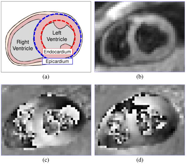
Short-axis DENSE CMR frame during contraction in a healthy human subject. (a) Anatomy, (b) magnitude, (c) horizontally encoded phase, and (d) vertically encoded phase.

Each phase pixel occupied by tissue is proportional to a displacement value indicating the location of the occupying tissue element when the DENSE encoding pulses were applied. Large phase values caused by large displacements are wrapped to the intrinsic MR phase range of [−π,π]. Phase wrapped pixels are visible in left ventricular tissue within the lateral wall (2 o’clock) of Fig. 1(c) and the anteroseptal wall (10 o’clock) of Fig. 1(d).

Practical DENSE encoding frequencies make phase unwrapping inevitable. It is possible to select a DENSE encoding frequency small enough so that no phase wrapping occurs; however, a reduction in the encoding frequency also reduces the sensitivity to displacement. Encoding frequencies in the region of 0.1 cycles/mm provide optimal results [41].

B. Motion Tracking

Tracking individual material points through time allows researchers and clinicians to easily visualize, quantify, and interpret tissue motion. However, cine DENSE observes displacement at fixed spatial locations through which the underlying tissue moves. Via the method outlined in [41], we are able to estimate the more easily interpreted material point trajectories from the observed DENSE displacements.

Horizontally and vertically encoded phase images are scaled and combined to produce a 2D displacement field [Fig. 2(a)]. Anatomy is manually delineated, eliminating extraneous displacement vectors [Fig. 2(b)]. Phase wrapping artifacts are corrected via a quality-guided path following unwrapping algorithm [49], evaluating and adjusting displacement values guided by the variance of local phase derivatives [Fig. 2(c)].

Fig. 2.

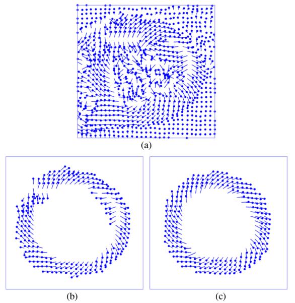
DENSE CMR displacement recovery. (a) Wrapped and un-segmented displacement vectors; cardiac displacement (b) before and (c) after unwrapping.

As illustrated in Fig. 2(c), the initial location of unwrapped DENSE displacement vectors (circular markers) are scattered throughout the initial cardiac configuration. Moreover, each frame of DENSE data refers to a unique set of tissue elements currently passing through the fixed imaging locations. Thus, to track an individual material point through the cardiac cycle, scattered displacements from each data frame must be interpolated for each material point origin.

A set of material points to track are selected from the initial tissue configuration, typically located at pixel centers. The location of each material point on every subsequent frame is estimated as a distance-weighted linear combination of nearby unwrapped displacement observations. As successive non view-shared cine DENSE images are independent, the accuracy of position estimates on each frame can be improved using estimates from other frames. Material point trajectories are thus fit to a fifth order Fourier series, previously shown to contain the majority of the energy of cardiac motion [50]. Fig. 3 illustrates a typical set of cardiac trajectories.

Fig. 3.

Cardiac trajectories in a healthy subject.

C. Strain Estimation

To gain additional insight into anatomical deformation, tissue strain is extracted from the tissue trajectories [51]. Tissue strain is a unit-less quantity defined as the relative change in tissue dimension from an undeformed state (e.g. the end-diastolic cardiac phase) to a deformed state (e.g. a phase in cardiac systole) [52], [53]. Positive strain indicates tissue lengthening, while negative strain indicates tissue shortening.

A multidimensional strain tensor can be estimated at each suitable material point of interest. Let t ∈ [0,1] represent time, ranging from the DENSE encoding pulse at t = 0 to the final frame acquisition at t = 1. Let ${\mathit{x}}_a\left(t\right)\in {\mathbb{R}}^2$ represent a spatial location within a deforming body at time t, where $a\in \left[1\dots \mathcal{A}\right]$. The distance vector between point a and neighboring point b at time t is given by

$${\delta }_{\mathit{ab}}\left(t\right)={\mathit{x}}_b\left(t\right)-{\mathit{x}}_a\left(t\right),$$ (1)

where $b\in \left[1\dots \mathcal{A}\right]$ and b ≠ a. The deformation gradient tensor F_a(t) characterizes the local deformation at point a as the body transforms through time. Provided tissue elements a and b are sufficiently close, F_a(t) is well approximated by

$${\delta }_{\mathit{ab}}\left(t\right)={\mathit{F}}_a\left(t\right)\cdot {\delta }_{\mathit{ab}}\left(0\right),$$ (2)

where δ_ab(0) and δ_ab(t) respectively represent the original and current tissue configurations. Given at least two suitable neighbors to point a, F_a(t) is determined via a least squares analysis. The strain tensor E_a(t) is related to F_a(t) by

$${\mathit{E}}_a\left(t\right)=\frac{1}{2}\left[{\mathit{F}}_a{\left(t\right)}^T{\mathit{F}}_a\right(t)-\mathbf{I}],$$ (3)

where I is the identity matrix.

To compare structures of arbitrary orientation, we perform an eigenvalue decomposition of the strain tensor [54]. This evaluates principle lengthening strain and principle shortening strain, defined as tissue strain in the directions of maximum and minimum dimensional change, respectively.

Fig. 4 illustrates typical mid-plane end-systolic principle shortening strain patterns in a healthy volunteer and patient with heart failure. A healthy subject’s heart typically has a predictable strain pattern, featuring relatively consistent strain values within each myocardial layer and a transmural strain gradient [55]. A patient’s heart can deviate from the expected strain pattern, e.g. the abnormal strain values around the septum of the left-ventricle (6 to 12 o’clock).

Fig. 4.

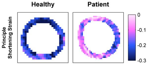
Human end-systolic principle strain patterns.

Fig. 5 illustrates regional mid-plane shortening strain curves in a healthy volunteer and patient with heart failure. Each curve represents the average strain within a specific region of the 17-segment American Heart Association cardiac model [56]. A healthy subject’s heart typically has predictable curve shapes that are consistent between regions. A patient’s heart can deviate from the typical curve shapes, e.g. the abnormal strain values in the anterior, anteroseptal, and inferoseptal cardiac segments.

Fig. 5.

Human principle shortening strain versus time curves.

D. Discussion

Though the standard cine DENSE analysis delivers informative motion and strain measurements, there are still opportunities for improvement:

• – As manual segmentation requires several minutes of user interaction per dataset (approximately 5 min per CMR slice), the analysis of multiple datasets quickly becomes tedious, time-consuming, and expensive. Recent work has attempted to speed segmentation, but still requires some user defined anatomy [43], [44].

• – Manual segmentation is nearly impossible early in the cine, as blood affected by the DENSE encoding pulse remains in the imaging plane and virtually eliminates tissue contrast.

• – Quality guided phase unwrapping has difficulty recovering true displacement values from un-segmented images containing multiple anatomical structures and regions devoid of tissue.

• – Distance-weighted linear interpolation offers little noise compensation and can result in unrealistic motion discontinuities.

The automated analysis solution presented in this article attempts to address and overcome each of these challenges.

III. Methods

In this section, we present our innovative algorithm to automatically track individual material points through space and time using noisy, wrapped, and un-segmented cine DENSE displacement observations.

A. General Notation

Before detailing our automated algorithm, we must first discuss some basic notation describing the problem. We then describe our problem in terms of this notation.

First, consider the cine DENSE acquisition space. Let t ∈ [0,1] represent time, ranging from the DENSE encoding pulse at t = 0 to the final image acquisition at t = 1; let t_i represent the temporal location of the i^th image frame, where $i\in \left[1\dots \mathcal{J}\right]$; and let ${\mathit{p}}_j\in {\mathbb{R}}^2$ represent the spatial location of the j^th image pixel, where $j\in \left[1\dots \mathcal{J}\right]$.

Next, consider the cine DENSE data. Let ${\overline{\Delta \mathit{u}}}_j\left[t_j\right]\in {\mathbb{R}}^2$ represent the potentially wrapped displacement vector observed at pixel j in frame i. Each component of the vector $\overline{\Delta \mathit{u}}$ satisfies $\mid \overline{\Delta \mathit{u}}\mid \le (.5∕k_e)$, where k_e is the DENSE encoding frequency in cycles per unit distance. The wrapped displacement $\overline{\Delta \mathit{u}}$ is related to the true displacement Δu by

$$\overline{\Delta \mathit{u}}=\mathrm{mod}(\Delta \mathit{u}+.5∕{\kappa }_e,1∕{\kappa }_e)-.5∕{\kappa }_e,$$ (4)

where mod(a, b) is the remainder after division of a by b. Thus, tissue underlying pixel j on frame i originated from the point u_j[t_i] = p_j – Δu_j[t_i].

Finally, consider a set of candidate material points to be tracked. Let ${\mathit{x}}_n\in {\mathbb{R}}^2$ represent the spatial location of the n^th material point at t = 0, where $n\in [1\cdots \mathcal{N}];\mathrm{let}\Delta x_n\left(t\right)\in {\mathbb{R}}^2$ represent the displacement of this material point away from the origin x_n; and let α_n represent a Boolean value indicating the presence of underlying tissue at this material point.

We may now suitably articulate the DENSE analysis problem. We must estimate the tissue extents {α_n} and spatiotemporal displacements {Δx_n(t)} of material points originating at locations {x_n} from the noisy, wrapped, and unsegmented DENSE displacement observations $\left\{\overline{\Delta {\mathit{u}}_j}\right[t_i\left]\right\}$ acquired at pixel locations {p_j} and times {t_i}.

Our solution to this problem is broken into two distinct stages. For each frame of data, we first unwrap displacement observations guided by previous motion estimates. We then estimate the displacement of material points occupied by tissue from the unwrapped observations.

B. Phase Unwrapping

In the first stage of our automated analysis method we unwrap displacement observations, predicting the current position of material points guided by prior material point motion, and estimating the true displacement underlying wrapped displacement observations consistent with these predictions.

Given a short interval between frame acquisitions, material points will likely experience only a small displacement between frames. We approximate the velocity of material point n on frame i according to

$${\mathit{v}}_n\left[t_i\right]\approx \frac{\Delta {\mathit{x}}_n\left[t_i\right]-\Delta {\mathit{x}}_n\left[t_{i-1}\right]}{t_i-t_{i-1}}.$$ (5)

Assuming material points continue to move with an approximately constant velocity over a small temporal interval, we may predict the displacement in frame i as

$$\Delta {\mathit{x}}_n^{⊛}\left[t_i\right]=\Delta {\mathit{x}}_n\left[t_{i-1}\right]+{\mathit{v}}_n\left[t_{i-1}\right]\cdot (t_i-t_{i-1}).$$ (6)

To safeguard against changes in material point topology (e.g. adjacent trajectories crossing paths in a physiologically impossible manner), displacement predictions are replaced with the median of themselves and immediate neighbors.

Informed by displacement predictions, we are able to correct phase wrapping artifacts. The true displacement vector underlying a wrapped observation is given by

$$\Delta {\mathit{u}}_j\left[t_i\right]={\overline{\Delta \mathit{u}}}_j\left[t_i\right]+{\xi }_j\left[t_i\right]\cdot (1∕{\kappa }_e),$$ (7)

where ξ_j[t_i] is a vector of unknown integers. To recover ξ_j[t_i], we must locate the m^th prediction closest to pixel j, minimizing the Euclidian distance $\Vert ({\mathit{x}}_m+\Delta {\mathit{x}}_m^{⊛}[t_i\left]\right)-{\mathit{p}}_j\Vert$ over values of $m\in \left[1\dots \mathcal{N}\right]$ for which α_m = 1. Assuming pixel j is occupied by tissue on frame i, the unwrapped observation is approximately equal to the closest displacement prediction. Thus, the vector ξ_j[t_i] can be recovered via

$${\xi }_j\left[t_i\right]=\text{round}[{\kappa }_e\cdot (\Delta {\mathit{x}}_m^{⊛}\left[t_i\right]-{\overline{\Delta \mathit{u}}}_j\left[t_i\right]\left)\right],$$ (8)

where the round(·) operator rounds values to the nearest integer.

The final step in the unwrapping processes quantifies the likelihood of tissue presence at each pixel. With respect to the DENSE phase data, pixels containing tissue typically observe an unwrapped displacement similar to the closest prediction. With respect to the DENSE magnitude data, pixels containing tissue typically observe a high/bright magnitude value. We quantify the likelihood that pixel j is occupied by tissue on frame i using both magnitude and phase data according to

$$L_j\left[t_i\right]=\mathit{exp}\left(-\frac{A_j{\left[t_i\right]}^2}{{{\ell }_A}^2}\right)\cdot \left[1-\mathit{exp}\left(-\frac{B_j{\left[t_i\right]}^2}{{{\ell }_B}^2}\right)\right],$$ (9)

where L ∈ [0,1], $A_j\left[t_i\right]=\Vert \Delta {\mathit{u}}_j\left[t_i\right]-\Delta {\mathit{x}}_m^{⊛}\left[t_i\right]\Vert$ is the difference between observed and predicted displacements, B_j[t_i] is the DENSE magnitude value, and l_A & l_B are positive scalars. Note this equation does not rely on magnitude data alone, as intravoxel dephasing can cause a decrease in pixel intensity.

Only displacement observations neighboring the current position of material points occupied by tissue need be considered. l_A is chosen to accommodate to the maximum expected change in material point velocity. For example, we select l_A = 1.0 for the human cardiac data discussed in Section IV.B to accommodate the initial velocity shift from rest to motion early in the cardiac cycle. When magnitude data is available, l_B is automatically selected for each DENSE magnitude image using Otsu’s method [57].

We consider pixel j to be likely devoid of tissue on frame i when L_j[t_i] is smaller than a threshold $\mathcal{L}\in [0,1]$, typically determined through a training set of DENSE data. For example, $\mathcal{L}=0.1$ successfully removes the majority of pixels unoccupied by tissue within the human cardiac data discussed in Section IV.B. The set of unwrapped displacement observations that survive the threshold are defined as {u_k[t_i]}, where $k\in \left[1\dots \mathcal{K}\right]$. Further discussion on parameter selection can be found in Section V.

C. Motion Estimation

In the second stage of our automated analysis method we estimate the true displacement of material points occupied by tissue from unwrapped displacement observations. This is accomplished via a well-established multivariate interpolation technique termed radial basis function interpolation, which guarantees the existence and uniqueness of an interpolation solution with only mild conditions on point geometry [58].

A radial basis function (RBF) ϕ(r) is a real-valued radially symmetric function depending only on the Euclidian distance from the origin. Global RBFs, such as the thin-plate spline [59], are real-valued within the entire interpolation space:

$${\varphi }_{\mathit{TPS}}\left(r\right)=r^2\log \left(r\right).$$ (10)

Local RBFs, such as the Gaussian RBF, shrink towards zero away from the origin:

$${\varphi }_{\mathit{GAU}}\left(r\right)=\exp (-r^2∕{\gamma }^2).$$ (11)

Compact support RBFs, such Wendland’s C² function [60], are equal to zero outside a specified support radius:

$${\varphi }_{\mathit{WC}2}\left(r\right)=\{\begin{array}{cc}\hfill {\left(1-\frac{r}{\beta }\right)}^4\left(4\frac{r}{\beta }+1\right)\hfill & \hfill r\le \beta \hfill \\ \hfill 0\hfill & \hfill r>\beta \hfill \end{array}\phantom{\}}.$$ (12)

A review of RBF choices for multivariate interpolation can be found in [61].

The RBF interpolant approximates an unknown function via a weighted sum of RBFs

$$g\left(\mathit{x}\right)=\sum _{k=1}^{\mathcal{K}}{\omega }_k\cdot \varphi (\Vert \mathit{x}-{\rho }_k\Vert ).$$ (13)

where g(x) is the function value at the point x, ϕ(∥x – ρ_k∥) is an RBF centered at the point ρ_k, and ω_k is the k^th basis function weighting factor. In some cases such as the thin plate spline, we add a first order polynomial to (13) to ensure a positive-definite solution.

RBF weights are determined through observations of the function g(·) at the points {ρ_k} according to

$$\Phi \omega =\mathit{G},$$ (14)

where $\omega ={\langle {\omega }_1\cdots {\omega }_{\mathcal{K}}\rangle }^T$ is a vector of RBF weights, $\mathit{G}={\langle g\left({\rho }_1\right)\cdots g\left({\rho }_{\mathcal{K}}\right)\rangle }^T$ is a vector of function observations, and an element of the 2D matrix Φ at row $r\in \left[1\dots \mathcal{K}\right]$ and column $c\in \left[1\dots \mathcal{K}\right]$ is given by Φ_rc = ϕ(∥ρ_r – ρ_c∥).

As the unwrapped displacement observations are in fact noisy, the exact interpolation condition of (14) is unwarranted. The interpolation condition may be relaxed [62] by instead minimizing the energy functional

$$E\left(\omega \right)=\lambda {\omega }^{\mathit{T}}\Phi \omega +\sum _{k=1}^{\mathcal{K}}{[{\Phi }_{\mathit{k}}\omega -g({\rho }_k\left)\right]}^2,$$ (15)

where Φ_k is the k^th row of the matrix Φ, and λ is a nonnegative scalar balancing functional smoothing and data interpolation. The RBF weighting factors minimizing this energy functional are defined by

$$(\Phi +\lambda \mathbf{I})\omega =\mathit{G},$$ (16)

where I is the identity matrix.

Through RBF interpolation we estimate material point displacement from the scattered displacement observations. We center an RBF at each spatial location u_k, and calculate RBF weights for each direction of displacement through the unwrapped displacement observations likely to contain tissue {Δu_k[t_i]} and (16). We then interpolate the displacements {Δx_n[t_i] of material points originating from locations {x_n} according to (13).

There are a number of factors to consider when selecting a specific RBF for interpolation. Global RBFs are able to estimate function values in regions lacking observations. The thin plate spline in particular is a popular RBF choice, featuring a rigorous mathematical underpinning as the fundamental solution to the biharmonic equation. Local RBFs more appropriately describe the local character of tissue motion, as observations have little effect on function estimates far from the observation. Compact support RBFs take the local operator to the logical extreme, as observations have no effect on function estimates outside the support region. Additionally, the limited extent of compact support RBFs generally results in a sparse constraint matrix Φ populated primarily with zeros, allowing for an efficient computation of RBF weights. For more information, a comprehensive analysis of RBF performance for general multivariate interpolation can be found in [61]. In Section IV, we will consider basis function and parameter selection in more detail.

Following interpolation, we determine if candidate material points are likely devoid of tissue. We average the current material point likelihood (initially set to one) and closest observation likelihood to obtain a new likelihood estimate. When this estimate drops below the threshold $\mathcal{L}$ discussed in the previous section, we consider the point likely devoid of tissue. Candidate material points not surviving the threshold are eliminated from further analysis by setting α_n to false.

D. Algorithm Summary

We may now summarize our algorithm for automatically tracking individual material points through space and time using noisy, wrapped, and un-segmented cine DENSE displacement observations.

We first initialize the material point origins {x_n} within the field of view, typically at the center of each pixel. Material point displacements and velocities are initially set to zero, i.e. Δx_n(0) = ν_n(0) = 0 for all n. As the tissue extents are initially unknown, we the likelihood of tissue presence to one and α_n to true for all n.

For each subsequent frame, we predict material point displacements $\left\{\Delta {\mathit{x}}_n^{⊛}\right[t_i\left]\right\}$ for all points where α_n is true, assuming a constant velocity between frames. We then estimate the true displacements {u_j[t_i]} from potentially wrapped observations $\left\{{\overline{\Delta \mathit{u}}}_j\right[t_i\left]\right\}$ guided by the predicted displacements.

We determine the likelihood of tissue presence {L_j[t_i]} for all observations using magnitude and phase data, selecting the magnitude parameter l_A via Otsu’s method [57] and the phase parameter l_B via the maximum expected change in material point velocity. Pixels with a likelihood smaller than the threshold $\mathcal{L}$, selected through training data, are likely devoid of tissue and are discarded. The set of unwrapped observations surviving the threshold is {u_k[t_i]}.

Through RBF interpolation, we estimate the true material point displacements {Δx_n[t_i]} from the unwrapped observations likely to contain tissue {u_k[t_i]}. Section IV.C provides details regarding the choice of basis function and interpolation parameters.

The current likelihood of tissue presence at each material point is averaged with the likelihood of tissue presence at the closest observation. Candidate material points not surviving the likelihood threshold $\mathcal{L}$ are considered devoid of tissue and are eliminated from further analysis by setting α_n to false.

After evaluating motion on all frames, we fit each surviving material point trajectory through time to a fifth order Fourier series. The entire process is repeated to refine motion estimates, making no further changes to the tissue extents {α_n} and replacing material point displacement predictions $\left\{\Delta {\mathit{x}}_n^{⊛}\right[t_i\left]\right\}$ with current displacement estimates {Δx_n[t_i]}.

Following motion estimation, principle strain patterns are calculated as per Section II.C and reported to the user.

IV. Results

In this section, we demonstrate the effectiveness of our fully automated algorithm for cine DENSE analysis using simulated and human CMR data. We first consider the selection of an appropriate radial basis function. We then validate the automated algorithm against the standard analysis method of Section II.B.

A. Simulated Data for Validation

100 normal and 100 abnormal short-axis cine DENSE CMR simulations were generated of an isolated left ventricle contracting in space. These simulations allowed for a direct evaluation of algorithm performance against exact knowledge of anatomical extents and tissue displacement.

1) Notation

Let t ∈ [0,1] represent time, ranging from the beginning to the end of the cardiac cycle. Let r = [r, θ]^T represent the polar coordinates of a material element in 2D space. This spatial transformation T(·) is given by

$$\left[\begin{array}{c}\hfill r^{\prime }\hfill \\ \hfill {\theta }^{\prime }\hfill \end{array}\right]=T(d,\phi ,\mathit{r})=\left[\begin{array}{c}\hfill r+d\hfill \\ \hfill \theta +\phi \hfill \end{array}\right],$$ (17)

where d and φ represent radial and angular displacement with respect to the polar origin r₀ = [0,0]^T.

2) Healthy data

The end-diastolic epicardial border and endocardial border are defined as concentric circles with constant radii R_ep and R_en centered on the polar origin r₀. These borders undergo a transformation to end-systole according to (17) via the parameters [d_ep, φ_ep] and [d_en,φ_en], respectively.

The end-systolic location of a left-ventricular material point originating from ${\mathit{r}}_n^{\mathit{ED}}$ is given by

$$\begin{array}{cc}\hfill {\mathit{r}}_n^{\mathit{ES}}& =T(d_n,{\phi }_n,{\mathit{r}}_n^{\mathit{ED}})\hfill \\ \hfill d_n& =[1-{\mu }_n]\cdot d_{\mathit{ep}}+{\mu }_n\cdot d_{\mathit{en}}\hfill \\ \hfill {\phi }_n& =[1-{\mu }_n]\cdot {\phi }_{\mathit{ep}}+{\mu }_n\cdot {\phi }_{\mathit{en}}\hfill \\ \hfill {\mu }_n& ={\left[\left(R_{\mathit{ep}}-r_n^{\mathit{ED}}\right)∕\left(R_{\mathit{ep}}-R_{\mathit{en}}\right)\right]}^{\sigma }\hfill \end{array}$$ (18)

where σ ∈ [0,∞) skews material point motion towards epicardial (σ > 1) or endocardial (σ < 1) motion. The displacement of this material point from its origin as a function of time is given by

$$\Delta {\mathit{r}}_n\left(t\right)=\Gamma \left(t\right)\cdot (r_n^{\mathit{ES}}-{\mathit{r}}_n^{\mathit{ED}}),$$ (19)

where Γ(t) ∈ [0,1] is the piece-wise continuous function illustrated in Fig. 6 derived from the standard left-ventricular volume diagram [63].

Fig. 6.

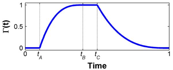
Simulated cardiac cycle weighting function.

3) Patient data

Abnormalities are introduced into a healthy motion field via

$$\begin{array}{cc}\hfill \Delta {\mathit{r}}_n\left(t\right)& =\Gamma \left(t\right)\cdot \left[\Psi \right({\theta }_n^{\mathit{ED}})\cdot {\mathit{r}}_n^{\mathit{ES}}-{\mathit{r}}_n^{\mathit{ED}}]\hfill \\ \hfill \Psi \left(\theta \right)& =\chi \cdot 0.5\cdot [1-\cos (\theta -\psi \left)\right]\hfill \end{array}$$ (20)

where the weighting function Ψ(θ) reduces tissue motion in the direction ψ ∈ [0,2π] by a factor χ ∈ [0,1].

End-systolic principle strain patterns derived from healthy and patient motion fields are shown in Fig. 7. Both simulations use identical simulation parameters, with the exception of the anterior defect in the patient simulation. Note the expected strain gradient in the healthy simulation, and a significant deviation from the expected strain pattern in the anterior region of the patient simulation.

Fig. 7.

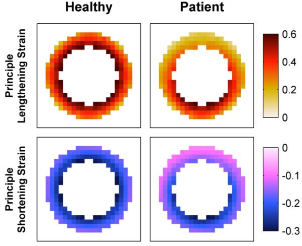
Simulated end-systolic principle strain patterns.

4) DENSE data

To simulate DENSE phase data for a given frame, we first sample left-ventricular displacement for that frame at a very high spatial resolution. The displacement observed at each pixel occupied by tissue is given by the average displacement of material points currently within the pixel bounds. Displacement observations are wrapped according to (4), scaled by the DENSE displacement encoding parameter, and split into separate phase images representing displacements in orthogonal directions.

Normally distributed phase noise is added to pixels occupied by tissue prior to wrapping. Tissue noise is increased with time, mimicking the time-dependent decrease in the signal-to-noise ratio (SNR) that is inherent to cine DENSE MRI. Pixels not occupied by tissue are given phase values of zero early in the cardiac cycle, mimicking blood affected by the DENSE encoding pulse within the imaging plane. These unoccupied pixels are given phase values uniformly distributed on the range [−π,π] later in the cardiac cycle. Fig. 8 illustrates a typical frame of simulated DENSE CMR data.

Fig. 8.

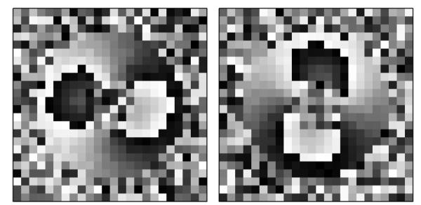
Simulated frame of DENSE CMR data; (left) horizontally and (right) vertically encoded phase.

5) Parameters

100 normal and 100 abnormal short-axis cine DENSE CMR simulations were generated. Each simulation utilized a unique set of physiological parameters:

– End-diastolic endo. radius ...........	$R_{\mathit{en}}~\mathcal{U}(10,30)\mathrm{mm}$
– End-diastolic wall thickness ........	$\tau ~\mathcal{U}(7.5,12.5)\mathrm{mm}$
– End-systolic endo. scaling ...........	$S_{\mathit{en}}~\mathcal{U}(0.6,0.8)$
– End-systolic area scaling .............	$S_{\mathit{ar}}~\mathcal{U}(0.9,1.1)$
– End-systolic endo. twist ..............	${\phi }_{\mathit{en}}~\mathcal{U}(-{10}^{\circ },+{10}^{\circ })$
– End-systolic epi. twist .................	φep = 0°
– Γ(t) parameters (Fig. 6) ..............	$t_A\sim \mathcal{U}(0.05,0.15)$
	$t_B\sim \mathcal{U}(0.35,0.45)$
	$t_C\sim \mathcal{U}(0.50,0.60)$
– Abnormal angle (if present) .......	$\psi \sim \mathcal{U}(0^{\circ },{360}^{\circ })$
– Abnormal scale (if present) .........	χ = 0.5

where $\mathcal{X}~\mathcal{U}(a,b)$ indicates a random value was selected for the variable $\mathcal{X}$ for each simulation from a uniform distribution on the range [a, b], R_ep = R_en + τ, d_en = (1 – S_en) R_en, and d_ep was calculated to achieve the requested change in left-ventricular area defined by s_ar. Imaging parameters included a [100×100] mm field-of-view at 3.0 mm/pixel, a 0.1 cycle/mm DENSE encoding frequency, and a 30 frame cine. Normally-distributed tissue noise increased linearly with respect to time, from a standard deviation value of 0.10 to 0.25 radians.

B. Human Data for Validation

2D cine DENSE CMR data were acquired in five healthy volunteers and five patients with heart failure using a 1.5T MR system (Avanto, Siemens). All subjects provided informed consent and all human studies were performed in compliance with protocols approved by our Institutional Review Board.

Healthy volunteers consisted of five male subjects ranging in age from 21 to 45, and patients consisted of two female and three male subjects ranging in age from 48 to 72. All five patients were diagnosed with heart failure, including conduction abnormalities such as left or right bundle branch block. Three patients had ischemic cardiomyopathy, and two had non-ischemic cardiomyopathy.

Each subject yielded three to four short-axis DENSE sequences extending from base to apex, totaling 32 unique short-axis sequences. Each healthy subject also yielded a two-chamber and four-chamber long-axis DENSE sequence, totaling 10 unique long-axis sequences.

Healthy subject imaging parameters included a [360×360] mm field-of-view at 2.8 mm/pixel, 8 mm slice thickness, 20° flip angle, 16 ms repetition time, 1.3 ms echo time, and a 0.1 cycle/mm DENSE encoding frequency [42]. Patient imaging parameters were identical except for a [350×350] mm field-of-view at 2.7 mm/pixel, 17 ms repetition time, and 1.08 ms echo time.

For comparison, tissue motion was estimated for each DENSE sequence using a semi-manual analysis technique described in [41] and outlined in Section II.B. Left-ventricular anatomy was manually delineated on one frame of each sequence by a trained technician and propagated to the remaining cine frames [43]. Anatomical outlines were fine-tuned by hand to ensure success of the quality-guided phase unwrapping algorithm. Material point trajectories originated from each pixel within the left-ventricular anatomy on the first frame of each sequence. As the distance-weighted linear (DWL) interpolation procedure has difficulty recovering tissue motion late in the cardiac cycle, motion estimates were not made for the last quarter of each sequence. Material point trajectories were fit to a fifth order Fourier series.

Principle strain maps were calculated from material point trajectories as described in Section II.C. Segmental strain-time curves were determined from these strain maps, averaging strain values on each frame within the standard 17-segment left-ventricular model of the American Heart Association [56]. Basal and mid-plane short-axis sequences were divided into six segments, apical short-axis sequences into four segments, and long-axis sequences into seven segments. Cardiac segments were delineated by hand.

C. Radial Basis Functions

In our first study, we considered the ability of radial basis functions to accurately estimate tissue motion and tissue strain. For this study we replicated the standard semi-manual analysis method of Section II.B, replacing DWL interpolation with RBF interpolation. To ensure a fair comparison, the same left-ventricular regions, unwrapped displacement vectors, and temporal fit orders were used for each interpolation technique.

We considered the three RBFs described in Section III.C: the thin-plate spline (10), Gaussian (11), and Wendland’s C² (12) function. RBF interpolation parameters were optimized with respect to human data, performing a global search of the parameter space for the best match of RBF to DWL motion estimates. The respective parameters for thin-plate spline, Gaussian, and Wendland’s C² interpolation were λ = 9.0, λ = 0.18 & β = 4 pixels, and λ = 0.18 & β = 11 pixels.

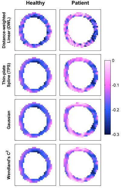
Fig. 9 and Fig. 11 illustrate typical end-systolic principle shortening strain maps in simulated and human datasets, respectively, derived using different interpolation methods. Simulated results are compared to the known strain pattern of Fig. 7, while human results are compared to DWL interpolation in Fig. 11.

Fig. 9.

End-systolic principle shortening strain patterns in simulated data using various interpolation methods.

Fig. 11.

End-systolic principle shortening strain patterns in human subjects using various interpolation methods.

For both simulated and human data, we report the root mean squared error (RMSE) between estimated and gold-standard material point positions. For human data, we also report linear regression and Bland-Altman analyses comparing estimated left-ventricular segmental strain estimates to the gold standard. When estimates are similar to the gold standard, the RMSE is low, linear regression reveals a slope and R² value near one, and Bland-Altman analysis reveals an average difference near zero with minimal spread.

We first evaluated RBF interpolation with respect to simulated data, comparing estimated to known material point positions. DWL, thin-plate spline, Gaussian, and Wendland’s C² interpolation respectively achieved an RMSE of 0.24 mm, 0.17 mm, 0.19 mm, and 019 mm (with respect to a maximum material point displacement of 11.3 mm).

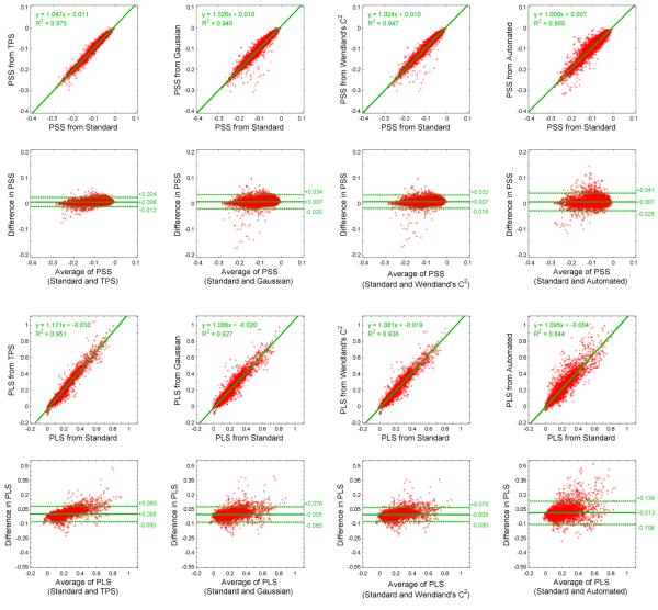
We then evaluated RBF interpolation with respect to human data, comparing estimated to gold standard motion and segmental strain. The values herein respectively compare thin-plate spline, Gaussian, and Wendland’s C² RBF interpolation to DWL interpolation across all datasets. The RMSE of all material point positions was 0.24 mm, 0.33 mm, and 0.30 mm (with respect to a maximum material point displacement of 18.4 mm). Fig. 13, columns 1-3, illustrates the comparison of segmental strain values. For principle shortening strain, linear regression revealed slopes of 1.05 (R²=0.95), 1.03 (R²=0.94) and 1.02 (R²=0.95); and Bland-Altman analysis revealed differences of 0.01±0.02, 0.01±0.03, and 0.01±0.03. For principle lengthening strain, linear regression revealed slopes of 1.17 (R²=0.95), 1.07 (R²=0.93), and 1.08 (R²=0.94); and Bland-Altman analysis revealed differences of 0.00±0.08, −0.01±0.08, and −0.01±0.08.

Fig. 13.

Comparison of segmental principle shortening strain (PSS) and principle lengthening strain (PLS) within human subjects.

All methods are compared to a standard semi-manual analysis using distance-weighted linear (DWL) interpolation.

Columns 1-3 consider semi-manual analyses using thin-plate spline (TPS), Gaussian, and Wendland’s C² radial basis function interpolation.

Column 4 considers the fully automated analysis presented within this article.

D. Automated Analysis

In our second study, we considered the ability of the proposed fully automated algorithm to accurately estimate tissue motion and tissue strain. The automated algorithm follows the procedure summarized in Section III.D. Material point trajectories were initialized at all pixel locations. Wendland’s C² function was selected for RBF interpolation as it provides both accurate interpolation results and an efficient implementation. Interpolation parameters were λ = 0.18 & β = 11 pixels, as determined in the previous section. Consider next the likelihood parameters of (9). For all data, we selected l_A = 1.0 to accommodate the initial velocity shift from rest to motion. For human data, l_B was automatically selected for each DENSE magnitude image via Otsu’s method [57], and we selected $\mathcal{L}=0.1$ through training experiments. As simulated data included no DENSE magnitude images, ${\ell }_B$ was set to zero and $\mathcal{L}$ was increased to 0.2.

Fig. 10 and Fig. 12 illustrate typical end-systolic principle shortening strain maps in simulated and human datasets, respectively, derived using the automated analysis. For improved visualization of cardiac function, the lower panels of these figures additionally highlight strain values within cardiac anatomy. Simulated results are compared to the known strain pattern of Fig. 7, while human results are compared to DWL interpolation in Fig. 11.

Fig. 10.

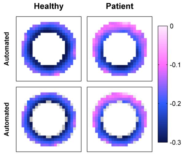
Automated end-systolic principle shortening strain patterns in simulated data, (top) without and (bottom) with highlighted anatomy.

Fig. 12.

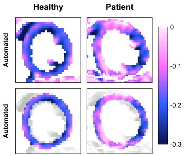
Automated end-systolic principle shortening strain patterns in human subjects, (top) without and (bottom) with highlighted anatomy.

We first evaluated the proposed technique with respect to simulated data, comparing estimated to known material point positions within the left ventricle. The automated algorithm achieved an RMSE of 0.20 mm (with respect to a maximum material point displacement of 11.3 mm), which is comparable to motion estimation methods that employ manual segmentation.

We next evaluated the proposed automated algorithm with respect to human data, comparing estimated to gold standard motion and segmental strain within the manually delineated left ventricle. The values herein compare the automated algorithm to semi-manual analysis using DWL interpolation across all datasets. The RMSE of all material point positions was 0.35 mm (with respect to a maximum material point displacement of 18.4 mm). Fig. 13, column 4, illustrates the comparison of segmental strain values. Linear regression and Bland-Altman analysis revealed a slope of 1.00 (R²=0.90), and difference of 0.01±0.03 for principle shortening strain and a slope of 1.10 (R²=0.84), and difference of 0.01±0.12 for principle lengthening strain.

V. Discussion

Results indicated good performance of RBF interpolation techniques, as discussed in Section IV.C. Simulated results showed good agreement between RBF interpolation and known tissue motion, and human results showed good agreement between RBF interpolation and the standard DWL interpolation technique. As evident in Fig. 9 and Fig. 11, strain patterns derived using RBF interpolation were similar overall to DWL interpolation, but were also smoother with a higher signal-to-noise ratio and no pixel discontinuities. RBF interpolation additionally clarified the expected transmural strain gradient in healthy subjects [55] as well as dysfunctional regions in patients with heart failure.

Results further indicated good performance of the proposed automated algorithm, as discussed in Section IV.D. Simulated results showed good agreement between the automated analysis and known tissue motion, and human results showed good agreement between the automated analysis and the standard semi-manual analysis technique. As evident in Fig. 10 and Fig. 12, the automated analysis maintained the expected transmural strain gradient in healthy subjects [55] and detected the dysfunctional regions in patient with heart failure. Most importantly, the automated algorithm provided access to high resolution tissue motion and tissue strain without the need for any user intervention. In both the clinical and research settings, this automation is critical to the future success of DENSE technology.

The automated algorithm incorporates several assumptions and parameter choices that must be addressed. Temporal resolution must be sufficient for the constant velocity motion model to provide acceptable estimates of frame-to-frame displacement. RBF parameters must be tuned to specific imaging conditions through representative training data, ensuring we maintain the ability to resolve small details in tissue function. Likelihood parameters must also be tuned through training data, as overly generous or overly conservative parameters may result in poor indications of tissue presence. It should be noted if improved knowledge of tissue presence is available, e.g. through another registered anatomical scan, this information could replace or be incorporated into the likelihood estimate. Finally, we must note the close coupling between likelihood estimates and RBF interpolation; a failure in one due to poor parameter choice will not likely be resolved by the other.

The automated algorithm does exhibit several limitations. Tissue bounds are often overestimated. For example, the endocardial and epicardial extents of simulated datasets were overestimated on the order of one pixel. Additionally, strain values can be misestimated at tissue-to-tissue interfaces. For example, principle lengthening strain can be overestimated within the inferior left-ventricular segments of short-axis human data due to neighboring stationary tissue. Finally, to compute regional strain versus time curves or to compute certain strain patterns such as radial and circumferential strain, users are still required to delineate anatomical extents from at least a single cine frame. Work is ongoing to improve tissue localization and automatically identify distinct anatomical structures.

The current implementation of the automated algorithm takes 2-4 minutes of processing time to complete a 20 frame sequence spanning [128×128] pixels. The most computationally consuming aspect of the algorithm is RBF interpolation, including both the computation of RBF weights and the interpolation of material point motion. Compact support RBFs offer the most efficient computation of RBF weights; in fact, computing global and local RBF weighting coefficients across the entire image is computationally prohibitive.

The speed of the automated algorithm is directly tied to the size of the assessed image region. The use of outer volume suppression (OVS) [30] to eliminate irrelevant image information far from anatomy of interest may prove very useful. OVS provides users the ability to quickly select a general image region containing the appropriate anatomy during scan setup, the preferred stage of acquisition and analysis for user input. Initial tests with OVS datasets have decreased execution time for a 20 frame sequence spanning [128×128] pixels to approximately 25 seconds.

Though far from trivial, an extension of the automated algorithm to recover 3D tissue motion from 3D cine DENSE data is fairly straightforward. The biggest obstacle is computational, as the number of DENSE observations increases exponentially from 2D to 3D. To recover 3D displacement in a reasonable timeframe, we will likely require additional automated analyses or user intervention to select a smaller volume containing structures of interest from the full field-of-view.

The automated algorithm has potential value to other tissue tracking technologies. Consider cine HARP, where tissue elements maintain invariant phase values which can be tracked through time. The proposed algorithm could be adapted to this technology to eliminate user intervention and improve error compensation, employing a similar strategy to predict material point displacement, locate suitable HARP observations, and interpolate true material point motion.

Future work will likely necessitate a comparison of the proposed algorithm with other automated analysis techniques across the spectrum of MR tissue tracking methods. Such a comparison, considering both the speed and accuracy of automated motion and strain recovery, is critical to the future success and acceptance of MR tissue tracking.

VI. Conclusion

Cine DENSE provides detailed measurements of tissue motion and tissue strain. Currently, motion analysis for these images relies on manually delineated anatomy. An automated analysis solution could improve measurement throughput, simplify data interpretation, and potentially access important physiological information during the imaging exam.

In this article, we presented the first fully automated solution for the estimation of tissue displacement and tissue strain from 2D cine DENSE data. Results using CMR data indicate good agreement between the automated algorithm and standard analysis methods. In a study of 42 unique cine DENSE CMR sequences from ten human subjects, Bland-Altman analyses revealed respective differences of 0.01±0.03 and 0.01±0.12 in principle shortening and lengthening strains between automated and standard analyses. This innovative and promising technique is an important step toward an automated cine DENSE analysis available for routine clinical use.

References

- [1].Zhong X, Epstein FH, Spottiswoode BS, Helm PA, Blemker SS. Imaging two-dimensional displacements and strains in skeletal muscle during joint motion by cine DENSE MR. Journal of biomechanics. 2008 Jan.vol. 41:532–40. doi: 10.1016/j.jbiomech.2007.10.026. [DOI] [PMC free article] [PubMed] [Google Scholar]
- [2].Soellinger M, Rutz AK, Kozerke S, Boesiger P. 3D cine displacement-encoded MRI of pulsatile brain motion. Magnetic Resonance in Medicine. 2009 Jan.vol. 61:153–62. doi: 10.1002/mrm.21802. [DOI] [PubMed] [Google Scholar]
- [3].Gotte MJW, van Rossum AC, Twisk JWR, Kuijer JPA, Marcus JT, Visser CA. Quantification of regional contractile function after infarction: strain analysis superior to wall thickening analysis in discriminating infarct from remote myocardium. Journal of the American College of Cardiology. 2001 Mar.vol. 37:808–817. doi: 10.1016/s0735-1097(00)01186-4. [DOI] [PubMed] [Google Scholar]
- [4].Bansal M, Cho G-Y, Chan J, Leano R, Haluska BA, Marwick TH. Feasibility and accuracy of different techniques of two-dimensional speckle based strain and validation with harmonic phase magnetic resonance imaging. Journal of the American Society of Echocardiography. 2008 Dec.vol. 21:1318–25. doi: 10.1016/j.echo.2008.09.021. [DOI] [PubMed] [Google Scholar]
- [5].Korosoglou G, Futterer S, Humpert PM, Riedle N, Lossnitzer D, Hoerig B, Steen H, Giannitsis E, Osman NF, Katus HA. Strain-encoded cardiac MR during high-dose dobutamine stress testing: comparison to cine imaging and to myocardial tagging. Journal of Magnetic Resonance Imaging. 2009 May.vol. 29:1053–61. doi: 10.1002/jmri.21759. [DOI] [PubMed] [Google Scholar]
- [6].Kramer CM, Magovern JA, Rogers WJ, Vido D, Savage EB. Reverse remodeling and improved regional function after repair of left ventricular aneurysm. Journal of Thoracic and Cardiovascular Surgery. 2002 Apr.vol. 123:700–6. doi: 10.1067/mtc.2002.120710. [DOI] [PubMed] [Google Scholar]
- [7].Setser RM, White RD, Sturm B, McCarthy PM, Starling RC, Young JB, Kasper J, Buda T, Obuchowski N, Lieber ML. Noninvasive assessment of cardiac mechanics and clinical outcome after partial left ventriculectomy. Annals of Thoracic Surgery. 2003 Nov.vol. 76:1576–85. doi: 10.1016/s0003-4975(03)00976-7. discussion 1585-6. [DOI] [PubMed] [Google Scholar]
- [8].Setser RM, Smedira NG, Lieber ML, Sabo ED, White RD. Left ventricular torsional mechanics after left ventricular reconstruction surgery for ischemic cardiomyopathy. Journal of Thoracic and Cardiovascular Surgery. 2007 Oct.vol. 134:888–96. doi: 10.1016/j.jtcvs.2007.05.060. [DOI] [PubMed] [Google Scholar]
- [9].Curry CW, Nelson GS, Wyman BT, Declerck J, Talbot M, Berger RD, McVeigh ER, Kass DA. Mechanical dyssynchrony in dilated cardiomyopathy with intraventricular conduction delay as depicted by 3D tagged magnetic resonance imaging. Circulation. 2000 Jan.vol. 101:E2. doi: 10.1161/01.cir.101.1.e2. [DOI] [PubMed] [Google Scholar]
- [10].Bilchick KC, Dimaano V, Wu KC, Helm RH, Weiss RG, Lima JA, Berger RD, Tomaselli GF, Bluemke DA, Halperin HR, Abraham T, Kass DA, Lardo AC. Cardiac magnetic resonance assessment of dyssynchrony and myocardial scar predicts function class improvement following cardiac resynchronization therapy. Journal of the American College of Cardiology. 2008 Sep.vol. 1:561–8. doi: 10.1016/j.jcmg.2008.04.013. [DOI] [PMC free article] [PubMed] [Google Scholar]
- [11].Castillo E, Lima JAC, Bluemke DA. Regional myocardial function: advances in MR imaging and analysis. Radiographics. 2003 Oct.vol. 23(Spec No):S127–40. doi: 10.1148/rg.23si035512. [DOI] [PubMed] [Google Scholar]
- [12].Ibrahim EH. Myocardial tagging by Cardiovascular Magnetic Resonance: evolution of techniques--pulse sequences, analysis algorithms, and applications. Journal of Cardiovascular Magnetic Resonance. 2011;vol. 13:36. doi: 10.1186/1532-429X-13-36. [DOI] [PMC free article] [PubMed] [Google Scholar]
- [13].Zerhouni EA, Parish DM, Rogers WJ, Yang A, Shapiro EP. Human heart: tagging with MR imaging--a method for noninvasive assessment of myocardial motion. Radiology. 1988;vol. 169:59–63. doi: 10.1148/radiology.169.1.3420283. [DOI] [PubMed] [Google Scholar]
- [14].Axel L, Dougherty L. MR imaging of motion with spatial modulation of magnetization. Radiology. 1989;vol. 171:841–845. doi: 10.1148/radiology.171.3.2717762. [DOI] [PubMed] [Google Scholar]
- [15].Mosher TJ, Smith MB. A DANTE tagging sequence for the evaluation of translational sample motion. Magnetic Resonance in Medicine. 1990;vol. 15:334–339. doi: 10.1002/mrm.1910150215. [DOI] [PubMed] [Google Scholar]
- [16].Fischer SE, McKinnon GC, Maier SE, Boesiger P. Improved myocardial tagging contrast. Magnetic Resonance in Medicine. 1993;vol. 30:191–200. doi: 10.1002/mrm.1910300207. [DOI] [PubMed] [Google Scholar]
- [17].Guttman MA, Prince JL, McVeigh ER. Tag and contour detection in tagged MR images of the left ventricle. IEEE Transactions on Medical Imaging. 1994 Jan.vol. 13:74–88. doi: 10.1109/42.276146. [DOI] [PubMed] [Google Scholar]
- [18].Chen T, Wang X, Metaxas D, Axel L. Fast Motion Tracking of Tagged MRI Using Angle-Preserving Meshless Registration. Medical Image Computing and Computer-Assisted Intervention. 2008:313–320. doi: 10.1007/978-3-540-85990-1_38. [DOI] [PubMed] [Google Scholar]
- [19].Smal I, Niessen W, Meijering E. Particle Filtering Methods for Motion Analysis in Tagged MRI. IEEE International Symposium on Biomedical Imaging; IEEE; 2010. [Google Scholar]
- [20].Smal I, Carranza-Herrezuelo N, Klein S, Wielopolski P, Moelker A, Springeling T, Bernsen M, Niessen W, Meijering E. Reversible jump MCMC methods for fully automatic motion analysis in tagged MRI. Medical image analysis. 2012 Jan.vol. 16:301–24. doi: 10.1016/j.media.2011.08.006. [DOI] [PubMed] [Google Scholar]
- [21].Osman NF, Kerwin WS, McVeigh ER, Prince JL. Cardiac motion tracking using CINE harmonic phase (HARP) magnetic resonance imaging. Magnetic Resonance in Medicine. 1999 Dec.vol. 42:1048–60. doi: 10.1002/(sici)1522-2594(199912)42:6<1048::aid-mrm9>3.0.co;2-m. [DOI] [PMC free article] [PubMed] [Google Scholar]
- [22].Osman NF, Prince JL. Visualizing myocardial function using HARP MRI. Physics in medicine and biology. 2000 Jun.vol. 45:1665–82. doi: 10.1088/0031-9155/45/6/318. [DOI] [PubMed] [Google Scholar]
- [23].Sampath S, Derbyshire JA, Atalar E, Osman NF, Prince JL. Real-time imaging of two-dimensional cardiac strain using a harmonic phase magnetic resonance imaging (HARP-MRI) pulse sequence. Magnetic Resonance in Medicine. 2003 Jul.vol. 50:154–63. doi: 10.1002/mrm.10509. [DOI] [PubMed] [Google Scholar]
- [24].Khalifa A, Youssef ABM, Osman N. Improved Harmonic Phase (HARP) Method for Motion Tracking a Tagged Cardiac MR images. IEEE International Conference of the Engineering in Medicine and Biology Society; 2005. pp. 4298–301. [DOI] [PubMed] [Google Scholar]
- [25].Liu X, Prince JL. Shortest path refinement for motion estimation from tagged MR images. IEEE Transactions on Medical Imaging. 2010 Aug.vol. 29:1560–72. doi: 10.1109/TMI.2010.2045509. [DOI] [PMC free article] [PubMed] [Google Scholar]
- [26].van Assen H, Florack L, Suinesiaputra A, Westenberg J. Purely Evidence Based Multiscale Cardiac Tracking Using Optic Flow. MICCAI Workshop on Computational Biomechanics for Medicine II.2007. pp. 84–93. [Google Scholar]
- [27].Florack L, van Assen H. A new methodology for multiscale myocardial deformation and strain analysis based on tagging MRI. International Journal of Biomedical Imaging. 2010 Jan. doi: 10.1155/2010/341242. [DOI] [PMC free article] [PubMed] [Google Scholar]
- [28].Osman NF, Sampath S, E EA, Prince JL. Imaging longitudinal cardiac strain on short-axis images using strain-encoded MRI. Magnetic Resonance in Medicine. 2001;vol. 46:324–334. doi: 10.1002/mrm.1195. [DOI] [PubMed] [Google Scholar]
- [29].Pan L, Stuber M, Kraitchman DL, Fritzges DL, Gilson WD, Osman NF. Real-time imaging of regional myocardial function using fast-SENC. Magnetic Resonance in Medicine. 2006 Feb.vol. 55:386–95. doi: 10.1002/mrm.20770. [DOI] [PubMed] [Google Scholar]
- [30].Ibrahim EH, Stuber M, Fahmy AS, Abd-Elmoniem KZ, Sasano T, Abraham MR, Osman NF. Real-time MR imaging of myocardial regional function using strain-encoding (SENC) with tissue through-plane motion tracking. Journal of Magnetic Resonance Imaging. 2007 Dec.vol. 26:1461–70. doi: 10.1002/jmri.21125. [DOI] [PubMed] [Google Scholar]
- [31].Ibrahim EH, Weiss RG, Stuber M, Spooner AE, Osman NF. Identification of different heart tissues from MRI C-SENC images using an unsupervised multi-stage fuzzy clustering technique. Journal of Magnetic Resonance Imaging. 2008 Aug.vol. 28:519–26. doi: 10.1002/jmri.21452. [DOI] [PMC free article] [PubMed] [Google Scholar]
- [32].Harouni AA, Bluemke DA, Osman NF. Fully automated segmentation of long-axis MRI Strain-Encoded (SENC) images using active shape model (ASM). IEEE International Symposium on Biomedical Imaging.2009. pp. 827–830. [Google Scholar]
- [33].Pelc LR, Sayre J, Yun K, Castro LJ, Herfkens RJ, Miller DC, Pelc NJ. Evaluation of myocardial motion tracking with cine-phase contrast magnetic resonance imaging. Investigative Radiology. 1994;vol. 29:1038–1042. doi: 10.1097/00004424-199412000-00005. [DOI] [PubMed] [Google Scholar]
- [34].Meyer FG, Constable RT, Sinusas AJ, Duncan JS. Tracking myocardial deformation using phase contrast MR velocity fields: a stochastic approach. IEEE Transactions on Medical Imaging. 1996;vol. 15:453–65. doi: 10.1109/42.511749. [DOI] [PubMed] [Google Scholar]
- [35].Jung B, Zaitsev M, Hennig J, Markl M. Navigator gated high temporal resolution tissue phase mapping of myocardial motion. Magnetic Resonance in Medicine. 2006;vol. 55:937–942. doi: 10.1002/mrm.20808. [DOI] [PubMed] [Google Scholar]
- [36].Arai AE, Gaither CC, III, Epstein FH, Balaban RS, Wolff SD. Myocardial velocity gradient imaging by phase contrast MRI with application to regional function in myocardial ischemia. Magnetic Resonance in Medicine. 1999 Jul.vol. 42:98–109. doi: 10.1002/(sici)1522-2594(199907)42:1<98::aid-mrm14>3.0.co;2-h. [DOI] [PubMed] [Google Scholar]
- [37].Cho J, Benkeser PJ. Cardiac segmentation by a velocity-aided active contour model. Computerized Medical Imaging and Graphics. 2006 Jan.vol. 30:31–41. doi: 10.1016/j.compmedimag.2005.10.006. [DOI] [PubMed] [Google Scholar]
- [38].Huntbatch A, Lee S-L, Firmin D, Yang G-Z. Bayesian Motion Recovery Framework for Myocardial Phase-Contrast Velocity MRI. Medical Image Computing and Computer-Assisted Intervention. 2008:79–86. doi: 10.1007/978-3-540-85990-1_10. [DOI] [PubMed] [Google Scholar]
- [39].Aletras AH, Ding S, Balaban RS, Wen H. DENSE: displacement encoding with stimulated echoes in cardiac functional MRI. Journal of Magnetic Resonance. 1999;vol. 137:247–52. doi: 10.1006/jmre.1998.1676. [DOI] [PMC free article] [PubMed] [Google Scholar]
- [40].Kim D, Gilson WD, Kramer CM, Epstein FH. Myocardial Tissue Tracking with Two-dimensional Cine Displacement-encoded MR Imaging: Development and Initial Evaluation. Radiology. 2004;vol. 230:862–871. doi: 10.1148/radiol.2303021213. [DOI] [PubMed] [Google Scholar]
- [41].Spottiswoode BS, Zhong X, Epstein FH, Hess AT, Kramer CM, Meintjes EM, Mayosi BM. Tracking myocardial motion from cine DENSE images using spatiotemporal phase unwrapping and temporal fitting. IEEE Transactions on Medical Imaging. 2007;vol. 26:15–30. doi: 10.1109/TMI.2006.884215. [DOI] [PubMed] [Google Scholar]
- [42].Zhong X, Spottiswoode BS, Meyer CH, Kramer CM, Epstein FH. Imaging three-dimensional myocardial mechanics using navigator-gated volumetric spiral cine DENSE MRI. Magnetic Resonance in Medicine. 2010 Jun.vol. 1097:1089–1097. doi: 10.1002/mrm.22503. [DOI] [PMC free article] [PubMed] [Google Scholar]
- [43].Spottiswoode BS, Zhong X, Lorenz CH, Mayosi BM, Meintjes EM, Epstein FH. Motion-guided segmentation for cine DENSE MRI. Medical Image Analysis. 2009;vol. 13:105–15. doi: 10.1016/j.media.2008.06.016. [DOI] [PMC free article] [PubMed] [Google Scholar]
- [44].Gilliam AD, Epstein FH, Acton ST. Cardiac motion recovery via active trajectory field models. IEEE Transactions on Information Technology in Biomedicine. 2009 Mar.vol. 13:226–35. doi: 10.1109/TITB.2008.2009221. [DOI] [PMC free article] [PubMed] [Google Scholar]
- [45].Haacke EM, Brown RF, Thompson M, Venkatesan R. Magnetic Resonance Imaging: Physical Principles and Sequence Design. J. Wiley & Sons; New York: 1999. [Google Scholar]
- [46].Aletras AH, Arai AE. meta-DENSE complex acquisition for reduced intravoxel dephasing. Journal of Magnetic Resonance. 2004 Aug.vol. 169:246–9. doi: 10.1016/j.jmr.2004.05.008. [DOI] [PubMed] [Google Scholar]
- [47].Epstein FH, Gilson WD. Displacement-encoded cardiac MRI using cosine and sine modulation to eliminate (CANSEL) artifact-generating echoes. Magnetic Resonance in Medicine. 2004;vol. 52:774–81. doi: 10.1002/mrm.20232. [DOI] [PubMed] [Google Scholar]
- [48].Zhong X, Spottiswoode BS, Cowart EA, Gilson WD, Epstein FH. Selective suppression of artifact-generating echoes in cine DENSE using through-plane dephasing. Magnetic Resonance in Medicine. 2006 Nov.vol. 56:1126–31. doi: 10.1002/mrm.21058. [DOI] [PubMed] [Google Scholar]
- [49].Ghiglia DC, Pritt MD. Two-Dimensional Phase Unwrapping: Theory, Algorithms and Software. Wiley-Interscience; New York: 1998. [Google Scholar]
- [50].Young AA. Epicardial deformations from coronary cineangiograms. In: Glass LL, Hunter P, McCulloch A, editors. Theory of Heart: Biomechanics, Biophysics, and Nonlinear Dynamics of Cardiac Function. Springer-Verlag; New York: 1991. [Google Scholar]
- [51].Truesdell C, Noll W. The Non-Linear Field Theories of Mechanics. Springer; New York: 2004. [Google Scholar]
- [52].Mirsky I, Parmley WW. Assessment of passive elastic stiffness for isolated heart muscle and the intact heart. Circulation Research. 1973 Aug.vol. 33:233–43. doi: 10.1161/01.res.33.2.233. [DOI] [PubMed] [Google Scholar]
- [53].Abraham TP, a Nishimura R. Myocardial strain: can we finally measure contractility? Journal of the American College of Cardiology. 2001 Mar.vol. 37:731–4. doi: 10.1016/s0735-1097(00)01173-6. [DOI] [PubMed] [Google Scholar]
- [54].Barbosa D, Claus P, Choi HF, Hristova K, Loeckx D, D’hooge J. An in-vivo study on the difference between principal and cardiac strains. IEEE International Ultrasonics Symposium.2009. pp. 1411–1414. [Google Scholar]
- [55].Moore CC, Lugo-Olivieri CH, McVeigh ER, Zerhouni EA. Three-dimensional systolic strain patterns in the normal human left ventricle: characterization with tagged MR imaging. Radiology. 2000 Feb.vol. 214:453–66. doi: 10.1148/radiology.214.2.r00fe17453. [DOI] [PMC free article] [PubMed] [Google Scholar]
- [56].Cerqueira MD, Weissman NJ, Dilsizian V, Jacobs AK, Kaul S, Laskey WK, Pennell DJ, Rumberger JA, Ryan T. Standardized Myocardial Segmentation and Nomenclature for Tomographic Imaging of the Heart: A Statement for Healthcare Professionals From the Cardiac Imaging Committee of the Council on Clinical Cardiology of the American Heart Association. Circulation. 2002;vol. 105:539–542. doi: 10.1161/hc0402.102975. [DOI] [PubMed] [Google Scholar]
- [57].Otsu N. A Threshold Selection Method from Gray-Level Histograms. IEEE Transactions on Systems, Man, and Cybernetics. 1979;vol. 9:62–66. [Google Scholar]
- [58].Buhmann MD. Radial Basis Functions: Theory and Implementations. Cambridge University Press; 2003. [Google Scholar]
- [59].Bookstein FL. Principal warps: Thin-plate splines and the decomposition of deformations. IEEE Transactions on Pattern Analysis and Machine Intelligence. 1989;vol. 11:567–585. [Google Scholar]
- [60].Wendland H. Scattered Data Approximation. Cambridge University Press; 2005. [Google Scholar]
- [61].de Boer A, van Der Schoot MS, Bijl H. Mesh deformation based on radial basis function interpolation. Computers & Structures. 2007;vol. 85:784–795. [Google Scholar]
- [62].Poggio T, Girosi F. Networks for approximation and learning. Proceedings of the IEEE. 1990;vol. 78:1481–1497. [Google Scholar]
- [63].McCulloch AD. Cardiac Biomechanics. In: Bronzino JD, editor. Biomedical Engineering Handbook. CRC Press LLC; Boca Raton: 2000. pp. 54.1–27. [Google Scholar]