

Abstract
Motivation: Reverse phase protein arrays (RPPA) measure the relative expression levels of a protein in many samples simultaneously. A set of identically spotted arrays can be used to measure the levels of more than one protein. Protein expression within each sample on an array is estimated by borrowing strength across all the samples, but using only within array information. When comparing across slides, it is essential to account for sample loading, the total amount of protein printed per sample. Currently, total protein is estimated using either a housekeeping protein or the sample median across all slides. When the variability in sample loading is large, these methods are suboptimal because they do not account for the fact that the protein expression for each slide is estimated separately.
Results: We propose a new normalization method for RPPA data, called variable slope (VS) normalization, that takes into account that quantification of RPPA slides is performed separately. This method is better able to remove loading bias and recover true correlation structures between proteins.
Availability: Code to implement the method in the statistical package R and anonymized data are available at http://bioinformatics.mdanderson.org/supplements.html.
Contact:sneeley@stats.byu.edu
Supplementary information: Supplementary data are available at Bioinformatics online.
1 INTRODUCTION
Protein arrays have been used in many contexts to measure protein expression in a high-throughput format (Becker et al. 2006; Grote et al. 2008; Hennessy et al. 2007; Herrmann et al. 2003; Kornblau et al., 2009; Kreutzberger 2006; Park et al. 2008). Assays that measure protein are able to address questions about post-translational modifications and protein pathway relationships that genomic studies alone cannot answer (Nishizuka et al. 2003b). Several different protein array formats have been developed, but they can be dichotomized into forward and reverse phase assays (Liotta et al. 2006). In forward phase arrays, numerous capture antibodies are printed on the array, which is then exposed to a single protein sample, allowing the simultaneous measurement of the level of multiple targets in a single sample. In reverse phase arrays, numerous protein samples are printed in discrete spots on the array, which is then probed with a single validated antibody, simultaneously measuring the level of a single protein in multiple samples. One reverse phase approach that uses lysed homogenized samples is the protein lysate or reverse phase protein array (RPPA) first described by Paweletz et al. (2001). Since then, RPPAs have been used by several groups worldwide to study the protein behavior in diseases (Chan et al. 2004; Herrmann et al. 2003; Jiang et al. 2006; Korf et al. 2008 Kornblau et al. 2009; Mendes et al. 2007; Park et al. 2008; Stevens et al. 2008; Zhang et al. 2009).
RPPAs have been used to address a number of biological questions. For example, RPPAs were used to study proteomic signatures of signaling pathways in various types of cancer including prostate (Grubb et al., 2003; Paweletz et al., 2001), breast (Akkiprik et al., 2006), glioma (Jiang et al., 2006), follicular lymphoma (Gulmann et al. 2005) and leukemia (Kornblau et al., 2009). Calvert et al. (2007), Nishizuka et al. (2003a) and Mendes et al. (2007) all found protein signatures that were able to distinguish between diseases or subtypes of disease. Other studies that use RPPAs to study proteins relating to pathway disregulation or drug response in cancer or other diseases include Ma et al. (2006); Wulfkuhle et al. (2003), Nishizuka et al. (2003b), Chan et al. (2004), Zha et al. (2004), Shankavaram et al. (2007) and Kim et al. (2008).
The RPPA assay is described in detail in Paweletz et al. (2001) (see also Charboneau et al., 2002; Espina et al. 2004; Liotta et al. 2006; Tibes et al. 2006). Briefly, biological samples are lysed, resulting in solutions that contain the protein of interest in unknown amounts. These sample lysates are spotted onto a nitrocellulose backed array in a dilution series. The array is then hybridized with a specific antibody validated to recognize only the protein of interest. Next, the array is incubated with a biotinylated secondary antibody that recognizes and binds to the primary antibody. Finally, streptavadin-linked labels (such as dyes) are introduced and bound to the biotin. When the array is processed, the labels can be observed and measured. It is assumed that the amount of label corresponds to the amount of protein at the spot. The processed arrays are scanned and the resulting images are analyzed with array software (we use MicroVigene®,VigeneTech, Carlisle, MA) that measures the foreground and background intensities of the label at each spot. RPPA ‘raw data’ consists of these measurements of foreground and background intensity at each spot on the array. Figure 1 shows an example of an RPPA slide with details of a few samples in their dilution series. The darker spots contain more protein than the lighter spots.
Fig. 1.

Image of an example RPPA with 1152 separate dilution series. Each dilution series is printed in 5-spot 1/2 dilutions. The zoom-in box shows 12 dilution series on the array. The darker the spot, the higher the amount of protein. Some of the spots do not appear on the array or in the zoom-in box because there was no label (i.e. protein) at the spot.
The reverse phase nature of RPPAs allows the levels of only one protein to be measured per array. Thus, RPPA experiments involve multiple arrays each printed identically with the same samples but probed with different antibodies. Such a set of arrays allows for estimation of sample effects that can go undetected with one array.
Similar to other array formats, this data undergoes a series of preprocessing steps before a formal analysis. The three main preprocessing steps are background subtraction, quantification and normalization. RPPA processing steps are performed sequentially:
Background correction: the background spot intensities are used to subtract baseline or non-specific signal from the foreground spot intensities.
Quantification: the background adjusted spot intensities from each dilution series are mapped into one number, the protein expression, that represents the amount of protein in the sample relative to the other samples on the array.
Normalization: the estimated relative sample expressions are adjusted to account for known sources of variation.
In this article, we focus on the normalization step. Specifically, we discuss current practices for estimating and correcting array and sample effects, with more focus on sample effects. We also propose a new normalization model that corrects array and sample effects based on the assumption that the protein expression estimates from each array are potentially on slightly different scales due to random variability in the quantification step.
Row and sample effects are assumed to be additive on the log scale:
| (1) |
where xjp is the estimated relative log expression in sample j on array p λj is the effect due to sample j δp is the effect due array p and cjp is the relative protein log expression with sample and array effects removed. Array effects are due to the fact that each array is quantified separately and protein expression is relative within slides. Sample effects occur when different amounts of total protein are unintentionally spotted on the array for different samples. Array and sample effects are further discussed in the next section.
The model we propose is a slight variation. The following simple modification to Equation (1) can improve normalized results when there is large variation in the sample effects:
| (2) |
Here, the γp term refers to a protein specific quantity that helps to account for error in estimating the sample protein expressions.
In order to motivate this model, we briefly discuss the quantification step. This is the only step that has been explicitly addressed in RPPA data (see Hu et al., 2007; Mircean et al., 2005;Nishizuka et al., 2003b; Tabus et al., 2006; and Supplementary Material).
The purpose of the quantification is to estimate the relative amount of protein in a sample as compared with the other samples on the same array using information from the dilution series and the observed intensities. This is accomplished by establishing a model relationship between the observed spot intensities and unknown relative expressions. Various groups have developed methods for RPPA quantification including models that use only sample information (Mircean et al., 2005; Nishizuka et al., 2003b) and ‘joint sample’ models that borrow strength from all samples on the array (Hu et al., 2007; Tabus et al., 2006). We use a joint sample model developed by our group at MD Anderson, called ‘SuperCurve’. This model is explained in detail in the Supplementary Material. Briefly, a three parameter logistic equation is used to model the dependency of the observed intensity on the unknown protein expression. There is one overall logistic curve estimated for the whole array and individual protein expressions are estimated as offsets from the overall curve. The logistic equation parameters and sample protein expressions are estimated iteratively (see Supplementary Material).
Sample protein expressions are estimated relative to the other samples on the array, and are reported without units. Since most estimation models, including SuperCurve, compute log expression values, in this article, we treat all expressions as on the log scale.
Array quantification is performed individually for each array. We have observed that this separate estimation of protein expression can result in unexpected multiplicative effects. For example, one experiment that we ran involved more samples than could be printed on a single array. We randomly allocated each sample to one of two groups, balancing for all potentially explanatory covariates that we could identify in advance. These two groups of samples were then printed on two parallel sets of arrays, which were interrogated with the same sets of antibodies. Due to the randomization, we knew that the distributions of protein expression for a given antibody should be the same for Groups 1 and 2. However, comparison of the expression distributions showed an unexpected shift in scale due to slightly different estimates of the slopes in the logistic curves used in the quantification of these arrays. These small differences are a result of error in the estimates of the logistic parameters. However, while the differences in slope estimates were slight, the range of sample loadings was broad, so the final expression estimates (and the protein clusters) were quite different. It is important to note that while this experiment (with samples split across arrays) first led us to identify the problem, these shifts in logistic slope are also present [and can be fixed with variable slope (VS) normalization] in the more common design context where all samples are printed on one array.
The usual normalization model in Equation (1) fails to capture the fact that protein expression is estimated separately for each slide and each array can have slightly different slopes in the overall logistic curve. Small errors in the slope parameter of the logistic curve can result in large variation if not properly accounted for.
The proposed model, Equation (2), adjusts for variability in slide-to-slide expression estimates when adjusting for sample loading. The γpterm refers to a protein-specific quantity that accounts for potentially differing slopes in the sigmoidal slope from the curve estimated with quantification methods described in Tabus et al. (2006), Hu et al. (2007) and the Supplementary Material. We call the new approach VS normalization because it accounts for variation in the estimated slope parameters from the calibration curve estimated in the quantification step.
2 METHODS
Normalization, using either Equations (1) or (2), requires estimation of both array and sample effects. Equation (2) additionally requires estimating multiplicative array effects. We first address additive array and sample effects and then the multiplicative array effects.
2.1 Array and sample effects
Array effects, δp in Equations (1) and (2), are actually common and even expected since each slide is quantified separately and expression estimates are relative within slides. These effects are corrected by normalizing expression to the median slide expression estimate so that each array has the same median expression.
Sample effects, λj, occur when the amount of total protein that is spotted on the array, the sample loading, varies from sample to sample. Unintentionally printing differing amounts of total protein for each sample can result in false conclusions of differential expression. Although efforts are made when the array is being printed to equalize total protein, this is often an unavoidable problem. For example, the same number of cells can be used in each biological sample, but if the size of the cells differs, then samples with larger cells will have more protein.
Sample loading has been estimated with a ‘housekeeping’ (HK) protein, such as β-Actin, as in Jiang et al. (2006) and Mendes et al. (2007). A HK protein is a protein that should be present in the same amount for all samples so differences in expression reflect differences in sample loading. However, in reality there is no protein that meets this expectation, and the expression levels of HK proteins can be quite variable. We refer to normalization with Equation (1), estimating λj with a HK protein, as HK normalization.
Another method that is used to estimate sample loading for the j-th sample is to use the median protein expression estimate for sample j across all the arrays, λj=medianj(xjp). This method assumes, first, that all the arrays were printed in a similar manner and, second, that most proteins will not be abnormally expressed but the few that are will still be noticed after normalization to the median. It is important to note that this method requires a set of arrays with the same samples. Normalization with Equation (1) but estimating λj with the median is called median loading (ML) normalization.
2.2 Multiplicative protein effects
The array-specific multiplicative effects, γp, in model 2 are partially confounded with the additive protein effects, δp. We outline a method that we have found to be effective in estimating parameters and performing sample loading normalization according to the VS normalization model.
First, write (2) as
| (3) |
The confounded term, δpγp, is lumped together as the overall protein effect and estimated with the median of protein p across all samples [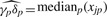 ]. Moving this term to the left-hand side, (3) can be written as
| (4) |
We will not be able to estimate the exact γp's, but taking the ratio of (4) for two values of p will allow estimation of the relative γp's. This ratio will be
| (5) |
where
since we assume that most cjp's will be small relative to λj. We also assume that the γp's have an expected value of 1 and a small variance. They should realistically have a range of around 0.5–1.5 so that there should not be a danger of ratios behaving badly as the denominator gets close to 0. We define  , hence Equation (5) implies that
  estimates the ratio γp1/γp2. This ratio can be estimated by regressing
  on
on  . Since there is no preferred direction (we could just as easily regress
  on
on  ) we use perpendicular least squares (de Groen, 1996; Rencher, 1995). The logs of these ratios are used to set up a system of equations whose solution yields estimates of the
  's: the system is made non-singular by setting
VS normalization is the process of adjusting the matrix  by dividing each column by the appropriate
  , and subtracting from each row the appropriate
  to obtain the estimate of cjp.
3 SIMULATIONS
We ran simulations to compare VS, ML and HK normalization. We randomly generated 30 proteins, each with 200 samples, from independent standard normal distributions. Array and samples effects were generated according to the following distributions, based on empirical data:
| (6) |
| (7) |
| (8) |
The ‘HK protein’ was modeled as:
| (9) |
In comparing the three methods, we wanted to assess the ability of each (i) to recover true protein correlation and (ii) to detect differential expression. To this end, two protein expression vectors were generated to have a correlation of 0.6, and another was ‘spiked’ with expression by adding a constant to one of the samples.
After each simulation, we performed normalization with the three methods and computed (i) correlation between correlated proteins and (ii) differential expression. Each target was compared with the truth using an estimated mean squared error ( ) defined as
| (10) |
where θ is the true value of the contrast (i.e. true correlation or true differential expression), and  is the value of the contrast for the i-th simulation.
Table 1 shows the  of the contrasts after 1000 simulations. The
  for VS normalization is better than both the other methods in every case and is good at maintaining correlation between proteins with known correlation.
Table 1.
Results of the simulation comparing the  s of HK, ML and VS normalization
| Contrast | HK MSE | ML MSE | VS MSE | Low MSE | |
|---|---|---|---|---|---|
| 1 | Correlated columns | 0.023 | 0.029 | 0.005 | 0.002 |
| 2 | Differential expression | 3.429 | 3.506 | 2.431 | 2.000 |
The theoretical minimum (Low) is also shown. We looked at two contrasts: (i) the correlation between two columns that should have a correlation of 0.6 and (ii) the difference between an unexpressed sample and a sample with spiked in expression (with a value of 5) within the same protein.
The last column of the table shows the ‘Lowest’  or what the
  would be if the parameters were known. This number is not 0 because of randomness in the data.
We performed a second set of simulations in which we varied the simulation parameters, including the number of proteins, the number of samples and the SDs of λj, δp and γp in Equations (6–8). The results of this simulations (shown in the Supplementary Material) similarly show that VS normalization performs as well or better than the other methods in all situations. The differences are most dramatic, however, when the variability in the sample loadings is large.
We ran a third simulation to compare only VS normalization with ML normalization when clustering proteins. We generated 30 proteins with 200 samples from a multivariate normal distribution with a covariance structure that allowed for five correlated groups as follows: Group 1, N=3, r=0.4; Group 2, N=10, r=0.2; Group 3, N=5, r=0.2; Group 4, N=5, r=0.5; and Group 5, N=7, r=0.3. The column, row and slope effects were generated according to Equations (6–8). Figure 2 shows a plot of the ‘true’, observed and normalized data matrices from a typical simulation.
Fig. 2.

The first two principal components plotted against each other for the true data matrix (A), the observed data matrix (B), the data matrix after ML normalization (C) and the data matrix after VS normalization (D). There are five groups each plotted in a different shade and symbol (every point represents a different protein/array). Each panel is shown in principal component space so rotation of axes is arbitrary; it is only important how the points group together. VS normalization is able to recover the group structure observed in the ‘true’ matrix, while ML normalization only recovers one of the groups.
It is easy to distinguish between groups for the true data, but grouping becomes scrambled after the row and column effects are introduced. ML normalization is able to separate some of the groups but still leaves many proteins scrambled. VS normalization is able to recover and separate all the groups present in the ‘true’ matrix. This example illustrates the strength of VS normalization to recover true correlation structure between proteins in the presence of high sample loading variability.
4 EXAMPLE WITH LEUKEMIA DATA
We applied the normalization methods to an RPPA experiment studying protein signatures in leukemia. A series of 138 lysate arrays were printed with either blood or marrow samples from 360 patients with acute lymphoblastic leukemia (ALL). Each sample was printed in duplicate on the array; each replicate was printed in a five spot, 2-fold dilution series. We used SuperCurve (see supplementary Material) to estimate protein expression for each dilution series.
The sample loadings for this data are quite variable. Figure 3 shows the protein expression for two extreme samples across all of the arrays. Figure 3A plots the expression before any loading normalization, showing that two samples can differ by nearly 8 U on a log 2 scale (a 256-fold difference) just due to sample loading. Figure (3B–D) plots protein expression for the same two samples after HK, ML and VS normalizations. There is still a slight loading bias after HK normalization, but the other two methods are able to correct this.
Fig. 3.
Protein expression for two extreme samples (a low expressed sample in black and a high expressed sample in gray) from an RPPA experiment with 138 slides. (A–D) The expression for the two samples across all arrays in the set. The array index is plotted on the x-axis and the estimated log expression is plotted on the y-axis. When there is no normalization, there is nearly an 8 log2 unit difference in expression (256-fold) between these samples primarily due to sample loading effects. HK normalization mostly corrects for sample loading, but there is still a 4-fold sample loading bias that the HK protein does not fix. Both median and VS normalization completely correct this level of observed sample loading bias. Note that there are differences in scale in each of the plots.
We performed hierarchical clustering of the 138 proteins, using average linkage for the linkage method and Pearson's correlation coefficient for the distance metric. For both VS and ML normalization methods, we checked the robustness of the protein clusters using bootstrap clustering (Kerr and Churchill, 2001; Pollard and van der Laan, 2005). HK normalization is excluded here because it did not remove all sample loading bias (Fig. 3). The idea behind bootstrap clustering is to see how often each pair of proteins clusters together in a set of bootstrapped samples. Based on the median split silhouette statistic (see (Pollard and van der Laan 2005), we assumed nine clusters. Figure 4 shows the results of a bootstrap cluster test with 500 bootstrapped samples after ML and VS normalizations. The figure ranges from perfectly yellow, meaning the proteins always cluster in the same group, to perfectly blue meaning the proteins never cluster in the same group (color version online). There are nine marginal colors that were assigned based on group membership of the proteins after the hierarchical cluster of the VS normalized data matrix. The colors in the margins of the plot are arbitrary, only used to illustrate change in group membership. The figure demonstrates that there is change in protein group membership depending on the normalization method used, confirming that the normalization approach is an important consideration. Although it is not possible to say which grouping is correct, the clusters found after VS normalization appear more robust, as seen by the tighter yellow squares along the diagonal.
Fig. 4.

Bootstrap Cluster results after ML (A) and VS normalization (B). The colors on the margin were assigned based on group membership after clustering the VS normalized data matrix. The marginal colors are present only to show that there is some shift in group membership depending on the normalization method. The clusters found after VS normalization seem to be more robust.
We attempted to determine which normalization method is most consistently correct. The ALL samples were each printed in duplicate on the array, so we performed hierarchical clustering with each set of replicates separately after both VS and ML normalization methods. Clustering with each replicate set should produce the same clusters, since the same set of samples is used. We counted the number of protein pairs that clustered together using the samples from one replicate but did not cluster together using the samples from the other replicate and divided this count by the total number of protein pairs. The count is interpreted as the percentage of protein pairs that did not cluster consistently. For the ALL samples from the set of 138 arrays, ML normalization inconsistently clustered 24% of the protein pairs while VS normalization inconsistently clustered 17% of the protein pairs. After filtering out non-informative samples, ML normalization inconsistency dropped to 18% and VS normalization inconsistency dropped to 12%. Both results are consistent with VS normalization as the preferred method.
5 DISCUSSION
Protein arrays are not currently in as widescale use as genomic arrays or other proteomic techniques; however, they are becoming more common. Several different groups have published analyses using RPPA technology (Gulmann et al. 2005; Hennessy et al. 2007; Jiang et al. 2006; Korf et al. 2008; Kornblau et al. 2009; Park et al. 2008; Tibes et al. 2006). Furthermore, RPPAs can be produced with common laboratory materials and techniques, making them more accessible than genomic arrays or mass spectrometry. As this technology becomes more common, appropriate preprocessing of the data will be even more important.
It is not a trivial problem to determine the best way or ways to normalize RPPA data. We have presented a traditional framework for correcting sample and array effects. We further introduced a slight modification to the standard procedure, the VS normalization method, which normalizes for total protein while taking into account error that can be introduced during the quantification step. Namely, since each array is quantified separately, slight variations in the estimated logistic slope of the dose response curve can create problems if ignored. The VS model better explains observed behavior and matches our knowledge of protein expression estimation. We have shown through simulation and an example with real data that how the VS method can recover true group correlations better than simply normalizing to the median of the samples or to a HK protein. We have also pointed out that the usual practice of normalization to a HK protein can be problematic both because of difficulties in finding a true HK protein and failures to remove all sample loading bias.
The impact of the multiplicative protein effect, γp in Equation (2), depends on variability in the sample loadings. Since the γp's are centered close to one, when the sample loadings have small variability, the impact of γp will also be small. However, the relatively small values of γp can have a large impact when variability in the sample loadings is large, as for example in the ALL data cited here. In these cases, it is especially important to correct for both additive and multiplicative protein effects. The type of sample contributes to how big the sample loading problem can be. Cell lines, for example, are not nearly as variable as tissue samples and usually do not have such large variations in sample loading across the samples.
The problem of sample loading is not something that can be resolved or even seen with just one array. Simulations not shown here suggest that at least 20 arrays (proteins) are adequate to provide good estimates of total protein, though fewer arrays can indicate a sample loading problem.
This is the first attempt that we know of to combine information across arrays in an RPPA study instead of focusing on each arrays individually.
Better estimation of the VS model parameters might be achieved with other estimation methods, such as with an iterative approach. In the future, we will investigate this possibility and how better estimates can improve results more. Although this procedure was developed for RPPAs, it can have application to any array assay in which different samples are printed together on the same array.
Conflict of Interest: none declared.
REFERENCES
- Akkiprik M, et al. Dissection of signaling pathways in fourteen breast cancer cell lines using reverse-phase protein lysate microarray. Technol. Cancer Res. Treat. 2006;5:543–551. doi: 10.1177/153303460600500601. [DOI] [PubMed] [Google Scholar]
- Becker K-F, et al. Clinical proteomics: new trends for protein microarrays. Curr. Med. Chem. 2006;13:1831–1837. doi: 10.2174/092986706777452506. [DOI] [PubMed] [Google Scholar]
- Calvert VS, et al. A systems biology approach to the pathogenesis of obesity-related nonalcholic fatty liver disease using reverse phase protein microarrays for multiplexed cell signaling analysis. Hepatology. 2007;46:166–172. doi: 10.1002/hep.21688. [DOI] [PubMed] [Google Scholar]
- Chan SM, et al. Protein microarrays for multiplex analysis of signal transduction pathways. Nat. Med. 2004;10:1390–1396. doi: 10.1038/nm1139. [DOI] [PubMed] [Google Scholar]
- Charboneau L, et al. Utility of reverse phase protein arrays: applications to signalling pathways and human body arrays. Brief. Funct. Genomic Proteomic. 2002;1:305–315. doi: 10.1093/bfgp/1.3.305. [DOI] [PubMed] [Google Scholar]
- de Groen PPN. An introduction to total least squares. Nieuw Arch. Wiskd. 1996;14:237. [Google Scholar]
- Espina V, et al. Protein microarray detection strategies: focus on direct detection technologies. J. Immunol. Methods. 2004;290:121–133. doi: 10.1016/j.jim.2004.04.013. [DOI] [PubMed] [Google Scholar]
- Grote T, et al. Validation of reverse phase protein array for practical screening of potential biomarkers in serum and plasma: accurate detection of CA19-9 levels in pancreatic cancer. Proteomics. 2008;8:3051–3060. doi: 10.1002/pmic.200700951. [DOI] [PMC free article] [PubMed] [Google Scholar]
- Grubb RL, et al. Signal pathway profiling of prostate cancer using reverse phase protein arrays. Proteomics. 2003;3:2142–2146. doi: 10.1002/pmic.200300598. [DOI] [PubMed] [Google Scholar]
- Gulmann C, et al. Proteomic analysis of apoptotic pathways reveals prognostic factor in follicular lymphoma. Clin. Cancer Res. 2005;11:5847–5855. doi: 10.1158/1078-0432.CCR-05-0637. [DOI] [PubMed] [Google Scholar]
- Hennessy B, et al. Pharmacodynamic markers of perifosine efficacy. Clin. Cancer Res. 2007;13:7421–7431. doi: 10.1158/1078-0432.CCR-07-0760. [DOI] [PubMed] [Google Scholar]
- Herrmann PC, et al. Mitochondrial proteome: altered cytochrome c oxidase subunit levels in prostate cancer. Proteomics. 2003;3:1801–1810. doi: 10.1002/pmic.200300461. [DOI] [PubMed] [Google Scholar]
- Hu J, et al. Nonparametric quantification of protein lysate arrays. Bioinformatics. 2007;23:1986–1994. doi: 10.1093/bioinformatics/btm283. [DOI] [PubMed] [Google Scholar]
- Jiang R, et al. Pathway alterations during glioma progression revealed by reverse phase protein lysate arrays. Proteomics. 2006;6:2964–2971. doi: 10.1002/pmic.200500555. [DOI] [PubMed] [Google Scholar]
- Kerr MK, Churchill GA. Bootstrapping cluster analysis: assessing the reliability of conclusions from microarray experiments. Proc. Natl Acad. Sci. USA. 2001;98:8961–8965. doi: 10.1073/pnas.161273698. [DOI] [PMC free article] [PubMed] [Google Scholar]
- Kim W, et al. A novel derivative of the natural agent deguelin for cancer chemoprevention and therapy. Cancer Prev. Res. 2008;1:577–587. doi: 10.1158/1940-6207.CAPR-08-0184. [DOI] [PMC free article] [PubMed] [Google Scholar]
- Korf U, et al. Quantitative protein microarrays for time-resolved measurements of protein phosphorylation. Proteomics. 2008;8:4603–4612. doi: 10.1002/pmic.200800112. [DOI] [PubMed] [Google Scholar]
- Kornblau S, et al. Functional proteomic profiling of AML predicts response and survival. Blood. 2009;113:154–164. doi: 10.1182/blood-2007-10-119438. [DOI] [PMC free article] [PubMed] [Google Scholar]
- Kreutzberger J. Protein microarrays: a chance to study microorganisms. Appl. Microbiol. Biotechnol. 2006;70:383–390. doi: 10.1007/s00253-006-0312-y. [DOI] [PMC free article] [PubMed] [Google Scholar]
- Liotta LA, et al. Protein microarrays: meeting analytical challenges for clinical applications. Clin. Cancer Res. 2006;12:4583–4589. doi: 10.1016/s1535-6108(03)00086-2. [DOI] [PubMed] [Google Scholar]
- Ma Y, et al. Predicting cancer drug response by proteomic profiling. Drug Discov. Today. 2006;11:1007–1011. [Google Scholar]
- Mendes KN, et al. Analysis of signaling pathways in 90 cancer cell lines by protein lysate array. J. Proteome Res. 2007;6:2753–2767. doi: 10.1021/pr070184h. [DOI] [PubMed] [Google Scholar]
- Mircean C, et al. Robust estimation of protein expression ratios with lysate microarray technology. Bioinformatics. 2005;21:1935–1942. doi: 10.1093/bioinformatics/bti258. [DOI] [PubMed] [Google Scholar]
- Nishizuka S, et al. Diagnostic markers that distinguish colon and ovarian adenocarcinomas: identification by genomic, proteomic, and tissue array profiling. Cancer Res. 2003;63:5243–5250. [PubMed] [Google Scholar]
- Nishizuka S, et al. Proteomic profiling of the NCI-60 cancer cell lines using new high-density reverse-phase lysate microarrays. Proc. Natl Acad. Sci. USA. 2003;100:14229–14234. doi: 10.1073/pnas.2331323100. [DOI] [PMC free article] [PubMed] [Google Scholar]
- Park M, et al. A quantitative analysis of N-myc downstream regulated gene 2 (NDRG 2) in human tissues and cell lysates by reverse-phase protein microarray. Clin. Chim. Acta. 2008;387:84–89. doi: 10.1016/j.cca.2007.09.010. [DOI] [PubMed] [Google Scholar]
- Paweletz CP, et al. Reverse phase protein microarrays which capture disease progression show activation of pro-survival pathways at the cancer invasion front. Oncogene. 2001;20:1981–1989. doi: 10.1038/sj.onc.1204265. [DOI] [PubMed] [Google Scholar]
- Pollard K, van der Laan MJ. Bioinformatics and Computational Biology Solutions Using R and Bioconductor. New York: Springer; 2005. pp. 209–228. ch. 13. [Google Scholar]
- Rencher AC. Methods of Multivariate Analysis. New York: John Wiley & Sons Inc.; 1995. [Google Scholar]
- Shankavaram UT, et al. Transcript and protein expression profiles of the NCI-60 cancer cell panel: an integromic microarray study. Mol. Cancer Ther. 2007;6:820–832. doi: 10.1158/1535-7163.MCT-06-0650. [DOI] [PubMed] [Google Scholar]
- Stevens E, et al. Predicting cisplatin and trabectedin drug sensitivity in ovarian and colon cancers. Mol. Cancer Ther. 2008;7:10–18. doi: 10.1158/1535-7163.MCT-07-0192. [DOI] [PubMed] [Google Scholar]
- Tabus I, et al. Nonlinear modeling of protein expressions in protein arrays. IEEE Trans. Signal Processing. 2006;54:2394–2407. [Google Scholar]
- Tibes R, et al. Reverse phase protein array: validation of a novel proteomic technology and utility for analysis of primary leukemia specimens and hematopoietic stem cells. Mol. Cancer Ther. 2006;5:2512–2521. doi: 10.1158/1535-7163.MCT-06-0334. [DOI] [PubMed] [Google Scholar]
- Wulfkuhle JD, et al. Signal pathway profiling of ovarian cancer from human tissue specimens using reverse-phase protein microarrays. Proteomics. 2003;3:2085–2090. doi: 10.1002/pmic.200300591. [DOI] [PubMed] [Google Scholar]
- Zhang L, et al. Serial dilution curve: a new method for analysis of reverse phse protein array data. Bioinformatics. 2009;25:650–654. doi: 10.1093/bioinformatics/btn663. [DOI] [PMC free article] [PubMed] [Google Scholar]
- Zha H, et al. Similarities of prosurvival signals in Bcl-2-positive and Bcl-2-negative follicular lymphomas identified by reverse phase protein microarray. Lab. Invest. 2004;84:235–44. doi: 10.1038/labinvest.3700051. [DOI] [PubMed] [Google Scholar]