Connectome‐scale assessments of structural and functional connectivity in MCI

Abstract

Mild cognitive impairment (MCI) has received increasing attention not only because of its potential as a precursor for Alzheimer's disease but also as a predictor of conversion to other neurodegenerative diseases. Although MCI has been defined clinically, accurate and efficient diagnosis is still challenging. Although neuroimaging techniques hold promise, compared to commonly used biomarkers including amyloid plaques, tau protein levels and brain tissue atrophy, neuroimaging biomarkers are less well validated. In this article, we propose a connectomes‐scale assessment of structural and functional connectivity in MCI via two independent multimodal DTI/fMRI datasets. We first used DTI‐derived structural profiles to explore and tailor the most common and consistent landmarks, then applied them in a whole‐brain functional connectivity analysis. The next step fused the results from two independent datasets together and resulted in a set of functional connectomes with the most differentiation power, hence named as “connectome signatures.” Our results indicate that these “connectome signatures” have significantly high MCI‐vs‐controls classification accuracy, at more than 95%. Interestingly, through functional meta‐analysis, we found that the majority of “connectome signatures” are mainly derived from the interactions among different functional networks, for example, cognition–perception and cognition–action domains, rather than from within a single network. Our work provides support for using functional “connectome signatures” as neuroimaging biomarkers of MCI. Hum Brain Mapp 35:2911–2923, 2014. © 2013 Wiley Periodicals, Inc.

INTRODUCTION

Mild cognitive impairment (MCI) refers to older adults who present with a mild degree of cognitive loss but do not meet the “NINDS/ADRDA” [Dubois et al., 2007; McKhann et al., 1984] diagnostic criteria for Alzheimer's disease (AD). As a precursor of AD with a progressive rate of as much as 15% [Grundman et al., 2004] each year, MCI also may show conversion to other neurodegenerative diseases [Petersen et al., 2001]. As a human‐specific disorder, even though it has been defined clinically [Albert et al., 2011; Sperling et al., 2011], accurate diagnosis of MCI and/or distinguishing it from other dementias or no cognitive impairment is still challenging.

Amyloid plaques, which are extracellular deposits of amyloid β and neurofibrillary tangles, are core pathological features of AD. Although amyloid PET imaging and measurement of beta‐amyloid (Aβ42) in cerebrospinal fluid have provided an indirect method for measuring fibrillar beta amyloid (Aβ) in the brain, these measures are difficult for clinical application due to their invasive nature. Also, the finding that many aged control and MCI brains exhibit a similar degree of Aβ deposition in postmortem brain tissues may limit the use of Aβ deposition as a biomarker for the distinguishing between normal aging and MCI patients [Aizenstein et al., 2008; Price et al., 2009]. Other biomarkers include gray matter (GM) atrophy which is often represented as changing of GM thickness [Wang et al., 2009], abnormality of white matter (WM) bundles [Li et al., 2008], and loss of volume with some specific brain tissues, such as in hippocampus, cingulate and entorhinal cortices [Devanand et al., 2007; Gómez‐Isla et al., 1996; Kordower et al., 2001; Mufson et al., 2012; Villain et al., 2010]. One limitation of the atrophy‐related biomarkers is that the changes in anatomical MRI typically are found later in the disease course. In addition, for MCI or early stages of AD, brain atrophy might be insignificant and spatially distributed over many brain regions [Chételat et al., 2002; Convit et al., 2000; Davatzikos et al., 2008; Dickerson et al., 2001].

Recently, researchers have begun to investigate the usefulness of resting‐state functional magnetic resonance (R‐fMRI) in studying differences between MCI/AD and normal controls [Greicius et al., 2004; Maxim et al., 2005; Sorg and Riedl, 2007; Supekar et al., 2008; Wang et al., 2007]. For example, Greicius [Greicius et al., 2004] suggested that a disruptive resting‐state activity exists within the default mode network (DMN) and decreased activity in the posterior cingulate and hippocampus can be detected in AD patients. Similarly, Sorg [Sorg and Riedl, 2007] found reduced functional interactions within DMN for MCI patients. Wang [Wang et al., 2007] implied decreased positive correlations usually exist between different lobes, such as prefrontal and parietal lobes; while increased positive correlations often appear within lobes. Supekar [Supekar et al., 2008] provided an early study examining the functional alterations to the brain network using small‐world properties. In general, R‐fMRI has an obvious advantage over traditional methods in MCI/AD‐related clinical applications due to its capability to reflect the intrinsic functional alternations occurring in the brain. However, compared to the previously mentioned biomarkers, fMRI‐based biomarkers are still much less well‐validated [Albert et al., 2011].

From our perspective, successful application of R‐fMRI data in MCI/AD studies has been hampered by two major barriers. First, there has been a critical lack of a common structural connectome that can serve as a universal brain reference system and structural substrate for functional/effective connectivity modeling. In essence, this has prohibited effective pooling, integration, comparison and validation of R‐fMRI derived biomarkers from different brains or populations. For instance, traditional brain functional connectivity (FC) studies often rely on anatomical parcellation or relatively large functional regions of interest (ROIs) as the nodes for functional network analysis. In parcellation cases, an individual brain is registered to a standard space (atlas) and multiple anatomical labels (from dozens to hundred) are obtained automatically [Wang et al., 2007]. In ROI analyses, nodes might come from functional computational modeling methods, such as DMN derived from ICA analysis [Sorg and Riedl, 2007]. One potential issue in these methods is that the BOLD signals are averaged within relatively large brain regions. Given the fact that larger ROIs (e.g., precentral gyri [BA 4] or medial prefrontal cortex in DMN) tend to contain multiple functional regions, averaging fMRI signals likely “smooth” out useful signals. Another problem is related to FC comparisons among different individuals. Indeed, registration can provide a rough correspondence but it may fail due to the significant variability of brain anatomical architecture. It is even more challenging to identify accurate mappings between populations with brain dysfunction, such as MCI, in that the structural and functional brain networks may have already been altered during disease progression. The second barrier is the critical lack of computational modeling strategies with which we can fuse, replicate and validate fMRI‐derived signatures in independent neuroimaging datasets. Validation of neuroimaging studies has been challenging for years due to the scarcity of ground‐truth data. It is even more challenging to validate on separate populations, given the variability in demographics, imaging equipment, scan protocols, image reconstruction algorithms and data preprocessing pipelines.

In this article, we propose a connectomes‐scale assessment of structural and FC for MCI patients via two independent multimodal diffusion tensor imaging (DTI)/fMRI datasets. Recently, we created and validated a novel data‐driven strategy that discovered 358 consistent ROIs with correspondences in over 200 brains. Each identified ROI was optimized to possess maximal group‐wise consistency of DTI‐derived fiber shape patterns. This set of 358 ROIs has been coined dense individualized and common connectivity‐based cortical landmarks (DICCCOL, http://dicccol.cs.uga.edu) [Zhu et al., 2012b]. To address the first barrier mentioned in this article, we adopted the DICCCOLs as predefined ROIs and tailored the abnormal ones relative to the normal controls. Those preserved DICCCOLs not only represent locations with similar structural connectivity profiles between MCI patients and normal controls but also ensure much finer granularity, better functional homogeneity, more accurate functional localization and automatically established cross‐subjects correspondence [Zhu et al., 2012b] during whole‐brain FC analysis. Another strategy that makes our method unique and efficient compared to previous studies is that we used two independent datasets in both the DICCCOL evaluation and the functional connectome‐based feature selection stages as a preliminary effort to overcome previous difficulties in validation and replication. We only consider the common DICCCOLs and the connectome features shared by both datasets after the DICCCOL tailoring and the two‐stage feature selection procedures, preserving and highlighting the most common characteristics of MCI subjects. Lastly, we introduced results of functional meta‐analysis [Yuan et al., 2013] to explore the most likely functional networks when analyzing the functional interactions for selected “connectome signatures.”

MATERIALS AND METHODS

Subjects

To infer and evaluate the common functional connectomes from MCI, two independent datasets from different research centers were used in this paper.

Dataset 1 included 28 participants with 10 MCI patients and 18 healthy controls. For image quality reasons, we selected 10 cases from healthy controls and all the MCI participants in this study. Participants were recruited and scanned in the Duke‐UNC Brain Imaging and Analysis Center (BIAC). Informed consent was obtained from all participants, and the experimental protocols were approved by Duke IRB. Criteria for MCI were in accordance with NACC procedures and NINCDS‐ADRDA diagnostic guidelines. Detailed inclusion and exclusion criteria have been reported in our previous work [Wee et al., 2011]. Confirmation of diagnosis for all subjects was made via expert consensus panels at the Joseph and Kathleen Bryan Alzheimer's Disease Research Center (Bryan ADRC) and the Department of Psychiatry at Duke University Medical Center. Diagnosis was based upon available data from a general neurological examination, neuropsychological assessment evaluation, collateral and subject symptom and functional capacity reports. Confirmation of the diagnosis for all subjects was made by a clinical psychiatrist at Duke Medical Center.

Dataset 2 included 24 older participants (ages 60+) at risk for MCI and/or dementia recruited from a 10‐county area around Athens‐Clarke County, Georgia. Initial recruitment was through advertisements and community contacts developed by the UGA Neuropsychology and Memory Assessment Laboratory. Informed consent was obtained upon initial recruitment into the study and the experimental protocol was approved by the UGA IRB. Participants completed comprehensive evaluations including MRI compatibility screening, participant and collateral interviews regarding relevant social and medical history by a trained interviewer certified in dementia rating, self and collateral reports of activities of daily living (ADLs) and neuropsychological testing. Information from the initial interview was used to make CDR staging decisions (group placement) according to CDR guidelines [Hughes et al., 1982]. Characteristics of the participants in two Datasets are summarized in Table 1.

Table 1.

Subject demographics for dataset 1 and dataset 2

	Mean ± standard deviation (range)
	Healthy controls	Patients with MCI
Dataset 1
Sample size	10	10
Male/female	1/9	5/5
Age (years)	67.7 ± 8.1 (55–82)	74.2 ± 8.6 (55–84)
Education (years)	16 ± 2.4 (12–20)	17.7 ± 4.2 (12–25)
MMSE	29.8 ± 0.4 (29–30)	28.4 ± 1.5 (26–30)a
Dataset 2
Sample size	12	12
Male/female	2/10	5/7
Age (years)	72.3 ± 5.1 (66–81)	78.1 ± 4.8 (68–84)
Education (years)	16.1 ± 2.6 (12–20)	14.7 ± 3.6 (5–18)
MMSE	28.3 ± 1.7 (25–30)	25.5 ± 2.5 (19–28)

^aMMSE score missing for one patient.

Imaging Data Acquisition

Dataset 1: The R‐fMRI and DTI datasets were acquired on a 3.0 T scanner (GE Signa EXCITE, GE Healthcare) at the Duke‐UNC BIAC. For DTI, 25 direction diffusion‐weighted whole‐brain volumes were acquired axially parallel to the AC–PC with b = 0 and 1,000. Major parameters include TR (repetition time) = 17 s, TE (echo time) = 78 ms and field of view (FOV) of 256 × 256 mm². The imaging resolution is 1 mm × 1 mm × 2 mm. For R‐fMRI imaging, the parameters are: 64 × 64 matrix, 3.8 mm slice thickness, 256 × 256 FOV, TR = 2 s and TE = 32 ms.

Dataset 2: The R‐fMRI and DTI datasets were scanned in a GE 3T Signa MRI system (GE Healthcare, Milwaukee, WI) at the UGA Bioimaging Research Center, Athens, GA. For DTI, 30 direction diffusion‐weighted whole‐brain volumes were acquired axially parallel to the AC–PC with b = 0 and 1,000. Major parameters include TR = 17 s, TE = min full and FOV of 256 × 256 mm². The imaging resolution is 2 mm isotropic. For R‐fMRI imaging, the parameters are: 64 × 64 matrix, 4 mm slice thickness, 256 × 256 FOV, TR = 5 s and TE = 25 ms.

Data Preprocessing

Preprocessing steps of the R‐fMRI data included brain skull removal, motion correction, spatial smoothing, temporal prewhitening, slice time correction, global drift removal and band pass filtering (0.01–0.1 Hz) [Li et al., in press; Zhu et al., 2012b]. Preprocessing steps of DTI data included brain skull removal, motion correction and eddy current correction. After preprocessing, fiber tracts, GM and WM tissue segmentation, GM/WM cortical surface reconstruction was performed based on the DTI data [Liu et al., 2007]. Fiber tracking was performed via MEDINRIA (http://www-sop.inria.fr/asclepios/software/MedINRIA/). Brain tissue segmentation was conducted on the DTI data directly [Liu et al., 2007]. Based on the WM tissue map, the cortical surface was reconstructed using the marching cubes algorithm [Liu et al., 2008]. The reconstructed surface has approximately 40,000 vertices and is used as the standard space for predicting DICCCOLs [Zhu et al., 2012b].

DICCCOL Prediction and Trace‐Map Filtering

Recently, we developed a novel data‐driven strategy that discovered 358 consistent ROIs with correspondence in six independent datasets of over 200 healthy brains. Each identified ROI was optimized to possess maximal group‐wise consistency of DTI‐derived fiber shape patterns. This set of 358 ROIs is referred to as Dense Individualized and Common Connectivity‐based Cortical Landmarks (DICCCOL http://dicccol.cs.uga.edu) [Zhu et al., 2012b]. In brief, through a group‐wise optimization process using a trace‐map model [Zhu et al., 2012a], 358 landmarks were stabilized from more than 2,000 candidates and each of them shown to have intrinsic correspondence across different individuals. During this procedure, only the WM bundles exactly penetrating or passing through a small neighborhood (radius = 2 mm) of the target location are considered. By adopting the prediction framework in [Zhu et al., 2012b], we can effectively transform the 358 DICCCOLs to a new brain. The prediction is similar to the DICCCOL optimization process: the consistency of the structural profiles between the new brain and the DICCCOL models will be maximized, as shown in Eq. (1).

$$E(S_{\mathrm{M}},S_{\mathrm{N}})=\sum \left|D_{\text{MN}}\right|.$$ (1)

S _M represents the DICCCOL models, S _N is the new brain that needs to be predicted, D _MN is defined as the trace‐map distance [Zhu et al., 2012a]. Briefly, trace‐map distance represents the similarity of the connectivity patterns between two separate WM (fiber) bundles. More details of the algorithms and results are referenced from our previous paper [Zhu et al., 2012b] and the website (http://dicccol.cs.uga.edu/).

However, considering that there could be alterations in structural/functional brain networks as revealed by DTI or R‐fMRI data within AD/MCI brains [Bozzali et al., 2002; Stebbins and Murphy, 2009; Supekar et al., 2008], there is a need to evaluate and tailor those discrepant DICCCOLs that deviate from those in healthy aged brains. We define the discrepant DICCCOLs as those having significantly higher trace‐map distances to the given models compared to the normal controls [Li et al., in press]. By setting the significance level as 0.05 (P‐value), we identified 56 and 95 abnormal DICCCOLs in dataset 1 and dataset 2, respectively. In the following steps in this article, we discarded those discrepant ones and only considered the DICCCOLs with similar distributions of trace‐map distance in both of the MCI subjects and healthy controls.

Functional Connectome Construction

Because fMRI and DTI sequences are both echo planar imaging sequences, their distortions tend to be similar and the misalignment between fMRI and DTI images is much less than that between fMRI and T1 images [Li et al., in press]. Thus, we adopted DTI space as the standard space for reporting the results. Coregistration between fMRI and DTI data was performed using FSL FLIRT. As the DICCCOLs are defined on the cortical surface (GM), we can significantly reduce the variance and noise [e.g., from WM and cerebrospinal fluid (CSF)] that are unlikely to reflect neuronal activities when we extract fMRI BOLD signals according to DICCCOLs. Therefore, for each preserved DICCCOL, we can effectively acquire its fMRI time series by averaging in a small neighborhood (three rings of surface mesh and the radius is approximate 3 mm). We evaluated the FC between each pair of DICCCOLs with Pearson correlation coefficients and constructed an M × M symmetric matrix for later analysis. Here, M equals the number of preserved DICCCOLs. For dataset 1, M = 302, and M = 263 for dataset 2.

Identification of Connections with High Differentiation Power

To some extent, the abnormal functional alterations in MCI can be represented by those FCs with highly discriminative power [Greicius et al., 2004; Sorg and Riedl, 2007; Wang et al., 2007]. Conversely, reducing the feature (e.g., paired correlation) numbers is an effective and sometime unavoidable way to accelerate the computation and reduce noise, including false positive correlations when only considering paired nodes. Hence, our strategy was to apply a two‐stage supervised feature selection procedure and only the features with the most distinctive and descriptive characteristics for differentiating MCI from healthy controls were preserved. In general, the first stage feature selection will find the common features shared by both datasets. The second stage will highlight those features specific to different populations.

As we only have two classes (MCI subjects and normal controls), we adopted a simple t‐test (P < 0.05) in the first stage to remove the connectivity without significant differences between two disease/control classes. However, the t‐test evaluates the features separately, which means it does not consider the relevance among the features and thus it cannot capture the redundancy of these preserved features. To tackle this problem, we used the correlation‐based feature selection (CFS) [Hall and Smith, 1999] algorithm as the second‐stage feature selection. The core idea of CFS is that through a heuristic process it evaluates the merit of a subset of features by considering the goodness of individual features for predicting the class along with the degree of intercorrelation among them. Unlike the first stage t‐test, CFS will compute feature–class and feature–feature correlations simultaneously. Given a feature subset S with k features, the Merit_s is defined as follows:

$${\text{Merit}}_{\mathrm{s}}=\frac{k\overline{\text{Corre}(\mathrm{c},\mathrm{f})}}{\sqrt{k+(k-1)\overline{\text{Corre}(\mathrm{f},\mathrm{f})}}},$$ (2)

where $\overline{\text{Corre}(\mathrm{c},\mathrm{f})}$ and $\overline{\text{Corre}(\mathrm{f},\mathrm{f})}$ are the mean feature–class correlation and the average feature–feature intercorrelation, respectively.

Support Vector Machine Classification and Cross‐Validation

Once we obtained the most common and discriminative connectivity following this two‐stage feature selection procedure, a support vector machine classifier [Chang and Lin, 2001] with linear kernel was used for solving the classification problem. Because of the limited numbers of subjects in the two datasets, we adopted the commonly used “leave‐one‐out” cross‐validation strategy to evaluate the sensitivity (proportion of patients correctly predicted) and specificity (proportion of healthy controls correctly predicted) of our selected features.

RESULTS

Discrepant DICCCOLs—Landmarks with WM Alterations in MCI

Many previous studies have shown that some structure alterations including GM loss and/or WM disruptions can be repetitively observed in MCI across different datasets and labs. For example, the hippocampus, cingulate [Risacher et al., 2009; Whitwell et al., 2007] and temporal lobe [Chételat et al., 2002; Frings et al., 2011] are believed to be brain structures involved in MCI/AD pathology, which can contribute to diagnostic accuracy [Barnes et al., 2004; Hanseeuw et al., 2011; Wahlund et al., 2005]. Diffusion tensor imaging has also revealed that several WM tracts are altered in MCI/AD, particularly in the corpus callosum (CC), cingulum bundle, fornix and uncinate fasciculus [Kiuchi et al., 2009; Li et al., 2008; Stricker et al., 2009]. As DICCCOLs are defined based on the group‐wise consistency of WM profiles, we hypothesized that the DICCCOLs related to those altered WM bundles would show different patterns between MCI patients and aged controls. In our experiment, after applying the DICCCOL prediction procedure [Zhu et al., 2012b] on MCI patients, some predicted DICCCOLs showed abnormal characteristics compared to the others. That is, these DICCCOLs displayed higher group trace‐map distances with MCI patients compared to the aged controls, indicating their fiber bundle patterns have higher variability at these locations. Using simple t‐tests to evaluate and explore those abnormal DICCCOLs that have significantly (P = 0.05) higher distributions of trace‐map distance in MCIs, we obtained 56 and 95 discrepant DICCCOLs for the two datasets. The results are illustrated in Figure 1.

Figure 1.

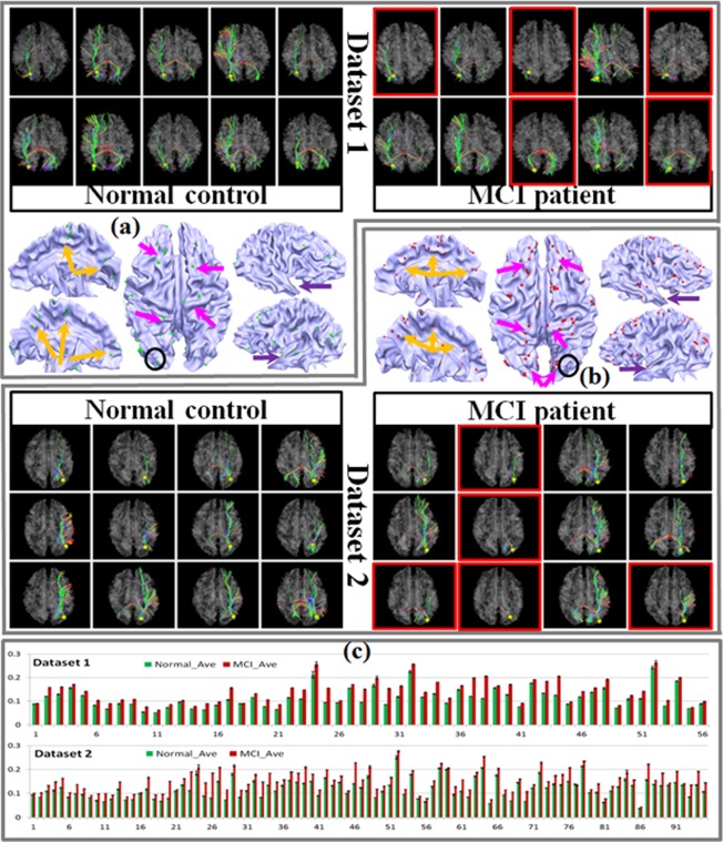
Discrepant DICCCOLs in two datasets. In total, we obtained 56 for dataset 1 and 95 for dataset 2. The discrepant DICCCOLs are displayed as colored bubbles on the cortex. We randomly chose one as an example and showed the WM bundles extracted from the selected DICCCOL on the top and bottom of (a) (dataset 1) and (b) (dataset 2). Some cases with significant differences between MCI subjects and normal controls are highlighted using red boxes. Subfigure (c) shows the comparison of trace‐map distance of the discrepant DICCCOLs between MCI and normal controls. [Color figure can be viewed in the online issue, which is available at http://wileyonlinelibrary.com.]

These discrepant DICCCOLs are plotted on the cortical surface using green and red bubbles (Fig. 1a,b) for two datasets, respectively. Although distributed over the whole cortex, they still show some clear assembling patterns and, as we expected, most of them are located in areas which are consistent with previous findings: orange and purple arrows show some DICCCOLs located at the cingulate region and entorhinal cortex [Devanand et al., 2007; Kordower et al., 2001; Risacher et al., 2009; Whitwell et al., 2007], respectively. The magenta arrows highlight the prefrontal areas [Morbelli et al., 2010] and dorsal part of the cortex which might be involved in the alteration of the CC [Kiuchi et al., 2009; Li et al., 2008; Stricker et al., 2009]. In general, the discrepant DICCCOLs are located near the regions that have previously been proved to be associated with atrophy/alteration of either GM or WM. One discrepant DICCCOL was randomly selected within each dataset and its corresponding fiber bundles were shown on the top and bottom of Figure 1a (dataset 1) and Figure 1b (dataset 2) as examples. The locations of the selected ones are marked with black circles. Examples of severely altered WM bundles of MCI patients are highlighted with red boxes. To quantitatively measure the difference of those discrepant DICCCOLs between MCI patients and aged controls, the average value and the standard deviation of the trace‐map distance within aged controls and MCI patients of the two datasets were calculated and are displayed in Figure 1c. From this visualization, we can see that the average trace‐map distances of MCI patients are significantly higher than those of aged controls (P < 0.05).

Note that as those discrepant DICCCOLs are no longer capable of providing consistent structural connectivity patterns, their intrinsic correspondences across different individuals are much less accurate. Hence in the following classification and functional network analysis, we discarded these discrepant DICCCOLs and constructed the functional connectomes only based on those “normal” DICCCOLs. However, those discrepant DICCCOLs may warrant further investigations and are mentioned in the discussion section.

Classification Results Based on Functional Connectomes

We summarized the number of preserved features at each feature selection stage and its corresponding classification results in Figure 2. In general, we had 45,451 and 34,453 features (pair‐wise FC) initially. After the first stage feature selection (t‐test) those features with no significant differentiation power were discarded and 2,106/3,691 connections passed through the significance test for Datasets 1 and 2, respectively. Interestingly, there were 134 common features across both datasets and they were treated as the input for the second‐stage feature selection (CFS). The feature training in the second stage was conducted within each dataset and all the subjects in the dataset were used for the training process. After that, we achieved 33 and 45 connectivity patterns for the two datasets (Table 2), which served as “connectomics signatures” for the subsequent disease/control classification and neuroscience interpretation. One important issue that should be noted is that some useful features may also be discarded in the first stage given the fact that a subset of features could have strong differentiation power together even if they could not pass the significance test alone. However, due to the computation power we did not utilize feature–feature relations given the large search space. Conversely, if these features made it through the first stage feature selection, they would be captured by the CFS (second stage) algorithm.

Figure 2.

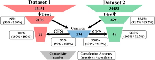
Summary of the feature selection procedure and the classification accuracy at each stage. [Color figure can be viewed in the online issue, which is available at http://wileyonlinelibrary.com.]

Table 2.

Summary of the “connectome signatures”

	Involved connectivity			Involved DICCCOLs
	Total	Increased	Decreased	Total	Action	Perception	Cognition	Emotion
Dataset 1	33	12	21	53	32/60.4%	33/62.3%	47/88.7%	32/60.4%
Dataset 2	45	44	1	67	41/61.2%	43/64.2%	56/83.6%	33/49.3%

To better demonstrate the advantages of our method, we reported not only the classification accuracy with the final feature set but also the number of survived connectivities and the intermediate classification results at each stage of the whole feature selection procedure. With the most relevant and discriminative connectivity selected, the classification accuracy substantially improved and we achieved 100% and 95.8% accuracies for the two datasets. Specifically, using the common (134, in total) FC of the t‐test results from the two datasets, the classification accuracy was not decreased (the accuracy did not change for dataset 1 and improved for dataset 2). This supports the feasibility of using common connectivity of different datasets to constrain the feature space in the following step. The functional networks involved in the finally preserved functional features (functional connectomes) were analyzed in the next section. Another interesting finding was that the same eight FC patterns survived in the final features of both datasets, which would be discussed later.

Functional Connectomes with High Differentiation Power

After two‐stage feature selection, we achieved 33 and 45 FCs which showed the most differentiation power (classification accuracy of 100% and 95.8%) for two datasets, hence we named them as “connectome signatures.” This section focuses on the functional roles/networks within these “connectome signatures.” Based on our previous work [Yuan et al., 2013; Zhu et al., 2012b], we successfully labeled DICCCOLs with corresponding functional roles (involved functional networks) through meta‐analysis. In brief, we registered the average coordinates of each DICCCOL to a standard atlas space and searched in a small range to check if any functional task activation reports for this location existed [Yuan et al., 2013]. If one or more activation reports were found in the considered range they were assigned to this DICCCOL as the corresponding functional roles. All the functional tasks (networks) used to label DICCCOLs were divided into five categories: action, perception, cognition, interoception and emotion (http://www.brainmap.org/sleuth/). For example, action includes eight subfunctional networks such as execution, imagination and inhibition. In total, we labeled 339 DICCCOLs with 55 subfunctional networks. Because few DICCCOLs involved in the “connectome signatures” are from the interoception network, we only considered the other four categories in this article. We quantitatively analyzed the composition of the acquired “connectome signatures” and the details are summarized in Figure 3. Not surprisingly, cognition‐related DICCCOLs played the most critical role within the signatures in both datasets. Those DICCCOLs involved in perception tasks also stood for a relatively high proportion.

Figure 3.

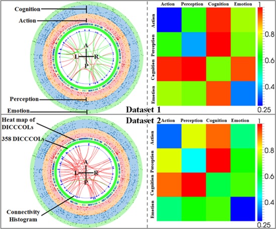
Representation of the derived “connectome signatures” (left) and their corresponding FRM (right). The green ticks in the middle ring indicate 358 DICCCOLs. The red and green curves represent increased and decreased connectivity, respectively. Connectivity histogram shows the degree of connectivity at a specific DICCCOL. Four colored rings in the outer layer represent four categories of functional networks: perception, action, cognition and emotion. The heat map between DICCCOLs and the functional network shows the total frequency of involvement in all the functional networks. [Color figure can be viewed in the online issue, which is available at http://wileyonlinelibrary.com.]

Figure 3 is a visual presentation of the “connectome signatures.” The green ticks in the middle ring indicate 358 DICCCOLs and they are roughly arranged according to the axial projection of the cortex surface: from top to bottom the ticks represent the DICCCOLs located at frontal, parietal, temporal and occipital lobes. The red and green curves represent increased and decreased connectivities, respectively. From the figure, we can see many increased ones (red curves) in both datasets. In fact in dataset 2, only one decreased connectivity exists. This result is consistent with previous studies [Grady and McIntosh, 2003; Grady et al., 2001; Wang et al., 2007] that increased connectivity is a common symptom in MCI and early stage AD, which is interpreted as a compensatory mechanism for reallocation or recruitment of cognitive resources to maintain routine performance in MCI/AD patients. Conversely, Wang et al. [2007] suggested that increased connectivity is mainly within the prefrontal lobe, parietal lobe and occipital lobe, whereas decreased connectivity is more likely found between the prefrontal and parietal lobes. Although our result of “connectome signatures” seems the opposite: decreased connectivity is found both within frontal lobe and between lobes (green curves of dataset 1); increased connectivity mainly exists between the lobes (red curves of dataset 1) and widely spread in the whole brain (red curves of dataset 2). The reasons leading to this seeming inconsistency might be twofold. (1) Previous studies reported all connectivity differences because they aimed to explore the distribution of the abnormal connections in different brain regions. Our results (Fig. 3), however, only show those selected connectivities with the most discriminative capability. In other words, many connectivity patterns with significant differences between normal/MCI are eliminated considering the information redundancy from the view of feature selection. (2) In this article, we adopted the DICCCOLs (after tailoring in the first step) as the predefined ROIs, which offer much finer granularity, better functional homogeneity, and more accurate functional localization [Zhu et al., 2012b], compared with those using Broadman areas. Another interesting observation of the “connectome signatures” is that the number of decreased connectivities in the two datasets is very different. One reason may be due to variability among the two datasets. An alternative explanation is the level of severity of the disease: the mini mental state examination (MMSE) score in Table 1 indicates that the MCI patients in dataset 2 are more severe than those in dataset 1. Another interesting finding is that there are eight common FC patterns of the “connectome signatures,” and most of them are increased ones. This suggests that compared to decreased connectivity, the increased ones are more general and robust for differentiating MCI/AD from normal participants. This set of common FC patterns was further analyzed in the next section.

Different from previous studies of FC [Supekar et al., 2008; Wang et al., 2007], in which only anatomical information is considered, our work extends it to the functional scope. As we have already functionally labeled each DICCCOL with a series of functional networks it is involved in, we can easily derive a Functional Relation Matrix (FRM) in the right column of Figure 3 as the representation of the “connectome signatures.” For example, there may exist a FC between DICCCOL‐A and DICCCOL‐B, in which DICCCOL‐A belongs to the functional network of action and perception and DICCCOL‐B belongs to perception only. As a consequence, this FC between two DICCCOLs will contribute to both action–perception and perception–perception relations in the matrix. Action–perception can be considered as a global‐scale interaction between different functional networks, while perception–perception can be identified as an intranetwork behavior. Even though we did not find much consistency from the connectivity directly, we can easily observe interesting patterns from the corresponding FRM: the number of FCs within any single functional network is very low, which is represented as the blue and green colors at the diagonal positions in Figure 3. Cognition–perception and cognition–action show significantly higher involvements in both datasets. These two consistent patterns suggest that those FCs that display the most differentiation power are mainly from the global‐scale interactions between different networks, rather than from within a single network. Here, it does not exclusively mean that the functional connections within a single functional network cannot help distinguish the patient (e.g., MCI/AD) from normal controls. For example, some previous studies already demonstrated that the disruption of the FCs within the DMN is an effective indicator for MCI/AD patients [Greicius et al., 2004; Sorg and Riedl, 2007].

Reproducible Connectivity Patterns in “Connectome Signatures”

It has been shown that the “connectome signatures” we achieved have remarkable classification performance within each dataset. As mentioned above, even though the involved FCs seem different between two datasets, they display a surprisingly consistent pattern in the functional space (FRM in Fig. 3). Therefore, we were very interested in whether there are certain FCs that are common across different datasets acquired from different research centers with different imaging settings. It is reassuring that there are eight common FCs (Fig. 4) in the “connectome signatures” of the two datasets, approximately 20% of the total FCs. Six of them showed consistent increased (red) connection and the other two common FCs displayed opposite (black) behavior across the two datasets. From the FRM, we can observe the high degree of involvement of cognition–perception interactions, and at the same time the internal functional interaction (diagonal grids) shows relatively low involvement in the “connectome signatures.” One point to be noted is that the two sets of “connectome signatures” survived from the two‐stage feature selection procedure and they already represent the most descriptive FCs between MCI patents and healthy controls. Hence, the common ones give us a view of which FCs are not only effective but also reproducible across different datasets. The six consistent FCs and their anatomical locations (via AAL atlas labels) are summarized in Table 3.

Figure 4.

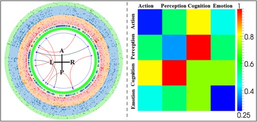
Representation of the common “connectome signatures” between two datasets and the corresponding FRM (right). [Color figure can be viewed in the online issue, which is available at http://wileyonlinelibrary.com.]

Table 3.

Anatomical regions involved in the six common and consistent “connectome signatures”

FC (DICCCOL‐DICCCOL)	Anatomical description
30–139	Occipital_Mid_R—Temporal_Inf_L
30–170	Occipital_Mid_R—Hippocampus_R
91–194	SupraMarginal_L—Amygdala_L
156–287	ParaHippocampal_L—Frontal_Inf_Orb_L
190–243	Temporal_Inf_L—Precentral_L
235–307	Frontal_Mid_L—Frontal_Sup_Medial_R

DISCUSSION AND CONCLUSION

Based on the DTI‐derived ROIs (DICCCOLs), we constructed whole‐brain functional connectomes and achieved efficient “connectome signatures” within each dataset. This study demonstrated that MCI patients can be distinguished from healthy aged controls by applying their own “connectome signatures” with high classification accuracy including both sensitivity and specificity. Even though some of the “connectome signatures” of the two datasets are different, their FRM exhibited highly consistent interaction patterns. The findings suggest that among those most discriminative FCs, the interactions between different functional networks were altered significantly, but the internal interactions within the networks do not change much compared to the normal controls.

In previous functional network analyses for the whole brain [Supekar et al., 2008; Wang et al., 2007; Zeng et al., 2012] including on normal controls or different brain conditions, the ROIs or nodes of the network are often constructed by registering the individual brain to the atlas space and the whole anatomically homogeneous region is treated as one functional unit. Then, the representative fMRI time‐series are acquired by averaging the BOLD fMRI signals within this relatively large brain area (the whole gyri or sulci in most cases). This framework works well when the goal is to explore the overall correlations between different anatomical regions, but it has limitations. As pointed out by Liu et al. [2008], the results of the whole‐brain FC might be affected by the BOLD signal's variability within the anatomical region of the atlas. Given a relatively large Brodmann area, such as the precentral gyrus, it is very likely that averaging the fMRI time‐courses of all voxels within the region might “smooth” out some useful signals and hence lose informative correlations in the follow‐up analysis. In comparison, the 358 DICCCOLs that are distributed over the whole cortex offer much finer granularity, better functional homogeneity, more accurate functional localization, and automatically established cross‐subjects correspondence [Zhu et al., 2012b]. Another advantage of the DICCCOL system is that it is defined on the cerebral cortical surface (GM), which makes it more accurate when extracting fMRI BOLD signals.

In this article, we discarded the discrepant DICCCOLs in which their WM connectivity patterns were altered significantly in an MCI population. Considering that these ignored landmarks represent the locations with high risk of structure abnormality, they could be more informative about the structural abnormality than the preserved ones. In the current stage, however, we have no better way to utilize these discrepant DICCCOLs for constructing statistical models because of the difficulty of building the correspondences among them across individuals. It could be beneficial to explore better approaches to examining these discrepant DICCCOLs in the near future. As a preliminary attempt, we isolated and showed the DTI‐fibers emitting from all the discrepant DICCCOL landmarks and the vertexes connected by this fibers in Figure 5. From the figure, we cannot find any obviously particular fiber bundles emitted from the discrepant DICCCOLs. Overall, it contains all the major tracts such as CC, inferior fronto‐occipital fasciculus and superior longitudinal fasciculus. In addition, we highlighted the surface vertexes that are affected by these discrepant‐DICCCOL fibers. Although some variation exists across different subjects, the affected areas tended to be widely spread over the whole cortex. These results seem to suggest that the WM/GM alterations in MCI tend to affect large areas in the brain.

Figure 5.

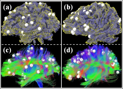
The DTI‐derived fibers emanating from all the discrepant DICCCOL landmarks and the surface vertices connected by this fibers. (a, c) and (b, d) show two examples. The white bubbles represent the discrepant DICCCOL landmarks and the fibers connecting to those DICCCOLs are shown in (c) and (d). The yellow dots demonstrated the regions affected by the displayed fibers. [Color figure can be viewed in the online issue, which is available at http://wileyonlinelibrary.com.]

Another potential limitation in our study was the variability of gender within the datasets used. Even though participants were originally selected according to well‐matched demographic variables including age and sex, discarding participant data because of limited image qualities either for DTI or fMRI data resulted in a larger number of female in normal controls of both datasets. Total sample sizes were also reduced and MCI patients were relatively older compared to the normal controls. However, recall that one of the advantages of our proposed method is the feasibility to fuse and combine different datasets from different labs, and this this potential issue can be dealt with by introducing extra datasets from a third party in the future.

In this study, we proposed a structural information‐guided FC analysis to assess and infer relevant functional connectomes for MCI patients. Based on the DICCCOL framework, we preserved those DICCCOLs without significant difference between MCI patients and normal controls. Then, through a two‐stage feature selection procedure, we obtained the most discriminative functional connectivities which we named “connectome signatures.” Our results indicate that: (1) these achieved “connectome signatures” have remarkable MCI‐vs‐controls classification accuracy (>95%); (2) even though some of the “connectome signatures” of the two datasets were different, their FRM exhibited highly consistent patterns. That is, the majority of “connectome signatures” mainly came from the interactions among different networks, for example, cognition–perception and cognition–action domains, instead of from a single network. Our work suggests high potential for using functional “connectome signatures” as neuroimaging biomarkers of MCI.

ACKNOWLEDGMENTS

The authors thank the anonymous reviewers for their constructive comments.

REFERENCES

- Aizenstein HJ, Nebes RD, Saxton JA, Price JC, Mathis CA, Tsopelas ND, Ziolko SK, James JA, Snitz BE, Houck PR, Bi W, Cohen AD, Lopresti BJ, DeKosky ST, Halligan EM, Klunk WE (2008): Frequent amyloid deposition without significant cognitive impairment among the elderly. Arch Neurol 65:1509–1517. [DOI] [PMC free article] [PubMed] [Google Scholar]
- Albert MS, DeKosky ST, Dickson D, Dubois B, Feldman HH, Fox NC, Gamst A, Holtzman DM, Jagust WJ, Petersen RC, Snyder PJ, Carrillo MC, Thies B, Phelps CH (2011): The diagnosis of mild cognitive impairment due to Alzheimer's disease: Recommendations from the National Institute on Aging‐Alzheimer's Association workgroups on diagnostic guidelines for Alzheimer's disease. Alzheimers Dement 7:270–279. [DOI] [PMC free article] [PubMed] [Google Scholar]
- Barnes J, Scahill RI, Boyes RG, Frost C, Lewis EB, Rossor CL, Rossor MN, Fox NC (2004): Differentiating AD from aging using semiautomated measurement of hippocampal atrophy rates. Neuroimage 23:574–581. [DOI] [PubMed] [Google Scholar]
- Bozzali M, Falini A, Franceschi M, Cercignani M, Zuffi M, Scotti G, Comi G, Filippi M (2002): White matter damage in Alzheimer's disease assessed in vivo using diffusion tensor magnetic resonance imaging. J Neurol Neurosurg Psychiatry 72:742–746. [DOI] [PMC free article] [PubMed] [Google Scholar]
- Chang C, Lin C (2001): LIBSVM: A library for support vector machines. Computer 2:1–30. [Google Scholar]
- Chételat G, Desgranges B, De La Sayette V, Viader F, Eustache F, Baron J‐C (2002): Mapping gray matter loss with voxel‐based morphometry in mild cognitive impairment. Neuroreport 13:1939–1943. [DOI] [PubMed] [Google Scholar]
- Convit A, De Asis J, De Leon MJ, Tarshish CY, De Santi S, Rusinek H (2000): Atrophy of the medial occipitotemporal, #inferior, #and middle temporal gyri in non‐demented elderly predict decline to Alzheimer's disease. Neurobiol Aging 21:19–26. [DOI] [PubMed] [Google Scholar]
- Davatzikos C, Fan Y, Wu X, Shen D, Resnick SM (2008): Detection of prodromal Alzheimer's disease via pattern classification of magnetic resonance imaging. Neurobiol Aging 29:514–523. [DOI] [PMC free article] [PubMed] [Google Scholar]
- Devanand DP, Pradhaban G, Liu X, Khandji A, De Santi S, Segal S, Rusinek H, Pelton GH, Honig LS, Mayeux R, Stern Y, Tabert MH, De Leon MJ (2007): Hippocampal and entorhinal atrophy in mild cognitive impairment: Prediction of Alzheimer disease. Neurology 68:828–836. [DOI] [PubMed] [Google Scholar]
- Dickerson BC, Goncharova I, Sullivan MP, Forchetti C, Wilson RS, Bennett DA, Beckett LA, deToledo‐Morrell L (2001): MRI‐derived entorhinal and hippocampal atrophy in incipient and very mild Alzheimer's disease. Neurobiol Aging 22:747–754. [DOI] [PubMed] [Google Scholar]
- Dubois B, Feldman H, Jacova C, Dekosky S, Barberger‐Gateau P, Cummings J, Delacourte A, Galasko D, Gauthier S, Jicha G, Meguro K, O'brien J, Pasquier F, Robert P, Rossor M, Salloway S, Stern Y, Visser P, Scheltens P (2007): Research criteria for the diagnosis of Alzheimer's disease: Revising the NINCDS‐ADRDA criteria. Lancet 6:734–746. [DOI] [PubMed] [Google Scholar]
- Frings L, Klöppel S, Teipel S, Peters O, Frölich L, Pantel J, Schröder J, Gertz H‐J, Arlt S, Heuser I, Kornhuber J, Wiltfang J, Maier W, Jessen F, Hampel H, Hüll M (2011): Left anterior temporal lobe sustains naming in Alzheimer's dementia and mild cognitive impairment. Curr Alzheimer Res 8:893–901. [DOI] [PubMed] [Google Scholar]
- Gómez‐Isla T, Price JL, McKeel DW, Morris JC, Growdon JH, Hyman BT (1996): Profound loss of layer II entorhinal cortex neurons occurs in very mild Alzheimer's disease. J Neurosci 16:4491–4500. [DOI] [PMC free article] [PubMed] [Google Scholar]
- Grady C, Furey M, Pietrini P, Horwitz B, Rapoport S (2001): Altered brain functional connectivity and impaired short‐term memory in Alzheimer's disease. Brain 124:739–756. [DOI] [PubMed] [Google Scholar]
- Grady C, McIntosh A (2003): Evidence from functional neuroimaging of a compensatory prefrontal network in Alzheimer's disease. J Neurosci 23:986–993. [DOI] [PMC free article] [PubMed] [Google Scholar]
- Greicius M, Srivastava G, Reiss A, Menon V (2004): Default‐mode network activity distinguishes Alzheimer's disease from healthy aging: Evidence from functional MRI. PNAS 101:4637–4642. [DOI] [PMC free article] [PubMed] [Google Scholar]
- Grundman M, Petersen RC, Ferris SH, Thomas RG, Aisen PS, Bennett DA, Foster NL, Jack CR, Galasko DR, Doody R, Kaye J, Sano M, Mohs R, Gauthier S, Kim HT, Jin S, Schultz AN, Schafer K, Mulnard R, Van Dyck CH, Mintzer J, Zamrini EY, Cahn‐Weiner D, Thal LJ (2004): Mild cognitive impairment can be distinguished from Alzheimer disease and normal aging for clinical trials. Arch Neurol 61:59–66. [DOI] [PubMed] [Google Scholar]
- Hall MA, Smith LA (1999): Feature selection for machine learning: Comparing a correlation‐based filter approach to the wrapper. Lloydia Cincinnati 235:239. [Google Scholar]
- Hanseeuw BJ, Van Leemput K, Kavec M, Grandin C, Seron X, Ivanoiu A (2011): Mild cognitive impairment: Differential atrophy in the hippocampal subfields. AJNR Am J Neuroradiol 32:1658–1661. [DOI] [PMC free article] [PubMed] [Google Scholar]
- Hughes CP, Berg L, Danziger WL, Coben LA, Martin RL (1982): A new clinical scale for the staging of dementia. Br J Psychiatry 140:566–572. [DOI] [PubMed] [Google Scholar]
- Kiuchi K, Morikawa M, Taoka T, Nagashima T, Yamauchi T, Makinodan M, Norimoto K, Hashimoto K, Kosaka J, Inoue Y, Inoue M, Kichikawa K, Kishimoto T (2009): Abnormalities of the uncinate fasciculus and posterior cingulate fasciculus in mild cognitive impairment and early Alzheimer's disease: A diffusion tensor tractography study. Brain Res 1287:184–191. [DOI] [PubMed] [Google Scholar]
- Kordower JH, Chu Y, Stebbins GT, DeKosky ST, Cochran EJ, Bennett D, Mufson EJ (2001): Loss and atrophy of layer II entorhinal cortex neurons in elderly people with mild cognitive impairment. Ann Neurol 49:202–213. [PubMed] [Google Scholar]
- Li S, Pu F, Shi F, Xie S, Wang Y, Jiang T (2008): Regional white matter decreases in Alzheimer's disease using optimized voxel‐based morphometry. Acta Radiol (Stockholm, Sweden: 1987) 49:84–90. [DOI] [PubMed] [Google Scholar]
- Li K, Zhu D, Guo L, Li Z, Lynch ME, Coles C, Hu X, Liu T: Connectomics signatures of prenatal cocaine exposure affected adolescent brains. Hum Brain Mapp (in press). doi:10.1002/hbm.22082. [DOI] [PMC free article] [PubMed] [Google Scholar]
- Liu T, Li H, Wong K, Tarokh A, Guo L, Wong STC (2007): Brain tissue segmentation based on DTI data. Neuroimage 38:114–123. [DOI] [PMC free article] [PubMed] [Google Scholar]
- Liu Y, Wang K, Yu C, He Y, Zhou Y, Liang M, Wang L, Jiang T (2008): Regional homogeneity, functional connectivity and imaging markers of Alzheimer's disease: A review of resting‐state fMRI studies. Neuropsychologia 46:1648–1656. [DOI] [PubMed] [Google Scholar]
- Maxim V, Sendur L, Fadili J, Suckling J, Gould R, Howard R, Bullmore E (2005): Fractional Gaussian noise, functional MRI and Alzheimer's disease. Neuroimage 25:141–158. [DOI] [PubMed] [Google Scholar]
- McKhann G, Drachman D, Folstein M, Katzman R, Price D, Stadlan EM (1984): Clinical diagnosis of Alzheimer's disease: Report of the NINCDS—ADRDA Work Group under the auspices of Department of Health and Human Services Task Force on Alzheimer's Disease. Neurology 77:939–944. [DOI] [PubMed] [Google Scholar]
- Morbelli S, Piccardo A, Villavecchia G, Dessi B, Brugnolo A, Piccini A, Caroli A, Frisoni G, Rodriguez G, Nobili F (2010): Mapping brain morphological and functional conversion patterns in amnestic MCI: A voxel‐based MRI and FDG‐PET study. Eur J Nucl Med Mol Imaging 37:36–45. [DOI] [PubMed] [Google Scholar]
- Mufson EJ, Binder L, Counts SE, DeKosky ST, De Toledo‐Morrell L, Ginsberg SD, Ikonomovic MD, Perez SE, Scheff SW (2012): Mild cognitive impairment: Pathology and mechanisms. Acta Neuropathol 123:13–30. [DOI] [PMC free article] [PubMed] [Google Scholar]
- Petersen RC, Stevens JC, Ganguli M, Tangalos EG, Cummings JL, DeKosky ST (2001): Practice parameter: Early detection of dementia: Mild cognitive impairment (an evidence‐based review). Report of the Quality Standards Subcommittee of the American Academy of Neurology. Neurology 56:1133–1142. [DOI] [PubMed] [Google Scholar]
- Price JL, McKeel DW, Buckles VD, Roe CM, Xiong C, Grundman M, Hansen LA, Petersen RC, Parisi JE, Dickson DW, Smith CD, Davis DG, Schmitt FA, Markesbery WR, Kaye J, Kurlan R, Hulette C, Kurland BF, Higdon R, Kukull W, Morris JC (2009): Neuropathology of nondemented aging: Presumptive evidence for preclinical Alzheimer disease. Neurobiol Aging 30:1026–1036. [DOI] [PMC free article] [PubMed] [Google Scholar]
- Risacher SL, Saykin AJ, West JD, Shen L, Firpi HA, McDonald BC (2009): Baseline MRI predictors of conversion from MCI to probable AD in the ADNI cohort. Curr Alzheimer Res 6:347–361. [DOI] [PMC free article] [PubMed] [Google Scholar]
- Sorg C, Riedl V (2007): Selective changes of resting‐state networks in individuals at risk for Alzheimer's disease. PNAS 104:18760–18765. [DOI] [PMC free article] [PubMed] [Google Scholar]
- Sperling RA, Aisen PS, Beckett LA, Bennett DA, Craft S, Fagan AM, Iwatsubo T, Jack CR, Kaye J, Montine TJ, Park DC, Reiman EM, Rowe CC, Siemers E, Stern Y, Yaffe K, Carrillo MC, Thies B, Morrison‐Bogorad M, Wagster MV, Phelps CH (2011): Toward defining the preclinical stages of Alzheimer's disease: Recommendations from the National Institute on Aging‐Alzheimer's Association workgroups on diagnostic guidelines for Alzheimer's disease. Alzheimers Dement 7:280–292. [DOI] [PMC free article] [PubMed] [Google Scholar]
- Stebbins GT, Murphy CM (2009): Diffusion tensor imaging in Alzheimer's disease and mild cognitive impairment. Behav Neurol 21:39–49. [DOI] [PMC free article] [PubMed] [Google Scholar]
- Stricker NH, Schweinsburg BC, Delano‐Wood L, Wierenga CE, Bangen KJ, Haaland KY, Frank LR, Salmon DP, Bondi MW (2009): Decreased white matter integrity in late‐myelinating fiber pathways in Alzheimer's disease supports retrogenesis. Neuroimage 45:10–16. [DOI] [PMC free article] [PubMed] [Google Scholar]
- Supekar K, Menon V, Rubin D, Musen M, Greicius MD (2008): Network analysis of intrinsic functional brain connectivity in Alzheimer's disease. PLoS Comput Biol 4:e1000100. [DOI] [PMC free article] [PubMed] [Google Scholar]
- Villain N, Fouquet M, Baron J‐C, Mézenge F, Landeau B, De La Sayette V, Viader F, Eustache F, Desgranges B, Chételat G (2010): Sequential relationships between grey matter and white matter atrophy and brain metabolic abnormalities in early Alzheimer's disease. Brain 133:3301–3314. [DOI] [PMC free article] [PubMed] [Google Scholar]
- Wahlund L‐O, Almkvist O, Blennow K, Engedahl K, Johansson A, Waldemar G, Wolf H (2005): Evidence‐based evaluation of magnetic resonance imaging as a diagnostic tool in dementia workup. Top Magn Reson Imaging 16:427–437. [DOI] [PubMed] [Google Scholar]
- Wang K, Liang M, Wang L, Tian L, Zhang X, Li K, Jiang T (2007): Altered functional connectivity in early Alzheimer's disease: A resting‐state fMRI study. Hum Brain Mapp 28:967–978. [DOI] [PMC free article] [PubMed] [Google Scholar]
- Wang L, Goldstein FC, Veledar E, Levey AI, Lah JJ, Meltzer CC, Holder CA, Mao H (2009): Alterations in cortical thickness and white matter integrity in mild cognitive impairment measured by whole‐brain cortical thickness mapping and diffusion tensor imaging. AJNR Am J Neuroradiol 30:893–899. [DOI] [PMC free article] [PubMed] [Google Scholar]
- Wee C‐Y, Yap P‐T, Li W, Denny K, Browndyke JN, Potter GG, Welsh‐Bohmer KA, Wang L, Shen D (2011): Enriched white matter connectivity networks for accurate identification of MCI patients. Neuroimage 54:1812–1822. [DOI] [PMC free article] [PubMed] [Google Scholar]
- Whitwell JL, Przybelski SA, Weigand SD, Knopman DS, Boeve BF, Petersen RC, Jack CR (2007): 3D maps from multiple MRI illustrate changing atrophy patterns as subjects progress from mild cognitive impairment to Alzheimer's disease. Brain 130:1777–1786. [DOI] [PMC free article] [PubMed] [Google Scholar]
- Yuan Y, Jiang X, Zhu D, Chen H, Li K, Lv P, Yu X, Li X, Zhang S, Zhang T, Hu X, Han J, Guo L, Liu T (2013): Meta‐analysis of functional roles of DICCCOLs. Neuroinformatics 11:47–63. [DOI] [PMC free article] [PubMed] [Google Scholar]
- Zeng L‐L, Shen H, Liu L, Wang L, Li B, Fang P, Zhou Z, Li Y, Hu D (2012): Identifying major depression using whole‐brain functional connectivity: A multivariate pattern analysis. Brain 135:1498–1507. [DOI] [PubMed] [Google Scholar]
- Zhu D, Li K, Faraco CC, Deng F, Zhang D, Guo L, Miller LS, Liu T (2012a): Optimization of functional brain ROIs via maximization of consistency of structural connectivity profiles. Neuroimage 59:1382–1393. [DOI] [PMC free article] [PubMed] [Google Scholar]
- Zhu D, Li K, Guo L, Jiang X, Zhang T, Zhang D, Chen H, Deng F, Faraco C, Jin C, Wee C‐Y, Yuan Y, Lv P, Yin Y, Hu X, Duan L, Hu X, Han J, Wang L, Shen D, Miller LS, Li L, Liu T (2012b): DICCCOL: Dense individualized and common connectivity‐based cortical landmarks. Cereb Cortex 23:786–800. [DOI] [PMC free article] [PubMed] [Google Scholar]