Nonlocal regularization of inverse problems: a unified variational framework

Abstract

We introduce a unifying energy minimization framework for nonlocal regularization of inverse problems. In contrast to the weighted sum of square differences between image pixels used by current schemes, the proposed functional is an unweighted sum of inter-patch distances. We use robust distance metrics that promote the averaging of similar patches, while discouraging the averaging of dissimilar patches. We show that the first iteration of a majorize-minimize algorithm to minimize the proposed cost function is similar to current non-local methods. The reformulation thus provides a theoretical justification for the heuristic approach of iterating non-local schemes, which re-estimate the weights from the current image estimate. Thanks to the reformulation, we now understand that the widely reported alias amplification associated with iterative non-local methods are caused by the convergence to local minimum of the nonconvex penalty. We introduce an efficient continuation strategy to overcome this problem. The similarity of the proposed criterion to widely used non-quadratic penalties (eg. total variation and `_p semi-norms) opens the door to the adaptation of fast algorithms developed in the context of compressive sensing; we introduce several novel algorithms to solve the proposed non-local optimization problem. Thanks to the unifying framework, these fast algorithms are readily applicable for a large class of distance metrics.

I. Introduction

The recovery of images from their few noisy linear measurements is an important problem in several areas, including remote sensing [1], biomedical imaging, astronomy [2], and radar imaging. The standard approach is to formulate the recovery as an optimization problem, where the linear combination of data consistency error and a regularization penalty is minimized. The regularization penalty exploits the apriori image information (eg.image smoothness [3], [4], transform domain sparsity [5]–[7]) to make the recovery problem well-posed.

Nonlocal means (NLM) denoising schemes have recently received much attention in image processing [8]–[10]. These methods exploit the similarity between rectangular patches in the image to reduce noise. Specifically, each pixel in the denoised image is recovered as a weighted linear combination of all the pixels in the noisy image. The weight between two pixels is essentially a measure of similarity between their patch neighborhoods (rectangular image regions, centered on the specified pixels) (see Fig.1). Recently, several authors have extended the non-local smoothing algorithm by reformulating it as a regularized reconstruction scheme. The regularization functional is the weighted sum of square differences between all the pixel pairs in the image [11]–[13]. The main challenge in applying this method to general inverse problems is the explicit dependence of the regularization penalty on pre-determined weights. In contrast to denoising and deblurring, good initial image guesses are often not available for many challenging inverse problems (eg. compressed sensing), which makes the reliable estimation of inter-pixel weights difficult. Some authors have suggested to iterate non-local schemes to improve the performance of deblurring and denoising algorithms; they re-estimate the weights from the current image iterate [14]–[16]. However, the use of this strategy to recover the image from its sparse Fourier samples results in the enhancement of alias patterns. Hence, this approach is not frequently used in such challenging inverse problems. Another limitation of current methods is that different optimization algorithms are required for each choice of regularization functional and weight [11], [14], [15], [17]; the algorithms designed for one penalty are often not readily applicable to other functionals.

Fig. 1.

Illustration of the proposed nonlocal framework: We illustrate the proposed regularization functional, specified by (13), in the left box. The regularization penalty is the sum of distances between patch pairs in the image.For each pixel x, we consider the distances between the patch centered at x (specified by Px(f)) and patches centered on the neighboring pixels y ∈ N_x; N_x is a square shaped window in which the algorithm searches for similar patches. We use the robust distance metric ϕ, which saturates with the the inter-patch distance. This property make the regularization penalty insensitive to large inter-patch distances, thus minimizing the averaging between dissimilar patches. The surrogate penalty, obtained by the majorization of G(f) in illustrated the right box. The surrogate penalty is essentially a weighted sum of Euclidean distances between pixel intensities. This criterion is very similar to the classical H₁ non-local penalty. The weights γ_fn (x, y) is obtained as the sum of the similarity measures as in (20). The similarity measures between patches are computed as a monotonically decreasing non-linear function (Ψ) of the inter patch distances. This property ensures that dissimilar patch pairs result in low inter pixel weights, thus encouraging the averaging of similar pixels.

To overcome the above mentioned problems, we introduce a unifying nonlocal regularization framework. We choose the regularization functional as an unweighted sum of non-Euclidean distances between patch pairs (see Fig. 1.a). We use robust distance metrics to promote the averaging of similar patches, while minimizing the averaging of dissimilar patches. Since the proposed criterion is not dependent on pre-estimated weights, the quality of the reconstructions is independent of the initial guess used for weight estimation. We show that a majorization of the proposed regularization penalty is very similar to current non-local regularization functionals [11], [14], [15], [17], when the robust distance metric is chosen appropriately. Thus, the fixed-weight NL schemes are similar to the first iteration of a majorize-minimize algorithm to solve the criterion. More importantly, the formulation provides a theoretical justification for the heuristic approach of iterating the NL algorithms by re-estimating the weights from the current image estimate [14], [15]. The availability of the global criterion, which does not change with iterations, enables us to analyze the convergence and design efficient algorithms; this approach is different from earlier methods that analyzed and optimized only one step of the above iterative scheme [11]–[15]. The practical benefits of the proposed reformulation are as follows:

• We now understand that the reason behind enhancement of alias artifacts, which are commonly reported in the context of current iterative weight update schemes, is caused by the convergence to the local minimum of the proposed criterion. We introduce homotopy continuation schemes to minimize such local minima problems, inspired by similar methods in compressed sensing [18]. Our experiments show that this approach eliminates the local minima issues in all the cases that we considered.

• The similarity of the proposed criterion to similar penalties in compressive sensing makes it possible to exploit the extensive literature in non-quadratic optimization (e.g. [19], [20]) to significantly improve computational efficiency. We introduce three majorize minimize (MM) algorithms, which rely on (a) the majorization of the penalty term (denoted as PM scheme), (b) the majorization of data term (indicated as DM algorithm), and (c) majorization of both data and penalty terms (termed as DPM scheme), respectively. Our experiments show that the PM scheme requires fewer computationally expensive weight computations and hence is computationally much more efficient than the DM and DPM schemes.

• Thanks to the unified perspective, it is possible to use the efficient PM algorithm for all non-local distance metrics. Previous methods required customized algorithms for each flavor of NL regularization.

The proposed framework is related to generalized nonlocal denoising schemes introduced in [21], [30]; they show that the iterative re-estimation of the weights results in improved reconstructions. However, the algorithms in [21], [30] are specifically designed for the denoising setting and are not applicable to general inverse problems, which is the main focus of this paper. This work is also related to convex patch based regularization scheme in [17], which is published in the same proceedings as the conference version of this paper [22]. The PM-CG algorithm provides faster convergence compared to DPM algorithm used in [17] (see the results section). In addition, we observe that non-convex nonlocal distance functions, along with homotopy continuation, provide significantly ameliorated results over the convex `₁ metric considered in [17].

II. Background

A. Current nonlocal algorithms

The classical NL means algorithm was originally designed for denoising. It derives each pixel in the denoised image as the weighted average of all the pixels in the noisy image¹f : Ω → ℝ:

$$\widehat{f}\left(\mathrm{x}\right)=\frac{{\Sigma }_{\mathrm{y}}w(\mathrm{x},\mathrm{y})\left(\mathrm{x}\right)}{{\Sigma }_{\mathrm{y}}w(\mathrm{x},\mathrm{y})}$$ (1)

The weight function w(x, y) is estimated from the noisy image or its smoothed version g as the similarity between the patch neighborhoods of the specific pixels:

$$w(\mathrm{x},\mathrm{y})=\exp \left(-\frac{\Vert P_{\mathrm{x}}\left(g\right)-P_{\mathrm{y}}\left(g\right){\Vert }_{\eta }^2}{{\sigma }^2}\right).$$ (2)

Here, P_x (g) is a (2Z_p + 1) × (2N_p + 1) image patch of g, centered at x:

$$P_{\mathrm{x}}\left(f\right)=f(\mathrm{x}+\mathrm{p});\mathrm{p}\in \underset{B_{\mathrm{x}}}{\overset{[-N_p,..N_p]\times [-N_p,..N_p]}{\underbrace{}}},$$ (3)

and ‖ · ‖ η denotes the weighted ℓ₂ metric defined as

$$\Vert f{\Vert }_{\eta }^2=\sum _{\mathrm{p}\in B_{\mathrm{x}}}\mid f\left(\mathrm{p}\right){\mid }^2\eta \left(\mathrm{p}\right).$$ (4)

B_x denote the pixels in the patch Px(f) and η(p) the window function. η is often chosen as a Gaussian function $(\eta \left(\mathrm{p}\right)=\exp (-\Vert {p\Vert }^2∕2N_p^2))$ to give more weight to the center pixel.

Recently, several authors have extended the nonlocal smoothing scheme [8]–[10] to deblurring and denoising problems by posing the image recovery as an optimization scheme [12], [13]:

$$\widehat{f}=\arg \underset{f}{\min }\Vert Af-b{\Vert }_2^2+\lambda J_w\left(f\right).$$ (5)

Here, the noisy measurements of the image are acquired by the ill-conditioned linear operator A. λ is the regularization parameter and J_w(f) is the nonlocal regularization functional. The subscript w is used to indicate that J_w(f) is explicitly dependent on pre-specified weights w. Several flavors of NL regularization penalties have been recently introduced. For example, H₁ nonlocal regularization uses the regularization functional:

$$J_{H_1}\left(f\right)=\sum _{\mathrm{x}\in \Omega }\sum _{\mathrm{y}\in N_{\mathrm{x}}}w\left(x,y\right)\mid f\left(\mathrm{x}\right)-f\left(\mathrm{y}\right){\mid }^2,$$ (6)

where the weights are specified as in (2). Note that the search window is restricted to the square neighborhood of x, denoted as N_x. This restriction is often used to keep the computational complexity manageable. Gilboa et. al., have suggested to replace the penalty term in (6) as

$$J_{\mathrm{TV}}\left(f\right)=\sum _{\mathrm{x}\in \Omega }\sum _{\mathrm{y}\in N_{\mathrm{x}}}w\left(x,y\right)\mid f\left(\mathrm{x}\right)-f\left(\mathrm{y}\right){\mid }^2,$$ (7)

while keeping the expression for the weights as in (2), to improve the quality of the reconstructions [11], [12]. This cost function is termed as nonlocal total variation (TV) penalty. Similarly, Peyre has introduced the regularization functional [15]:

$$J_{\mathrm{peyre}}\left(f\right)=\sum _{\mathrm{x}\in \Omega }\sum _{\mathrm{y}\in N_x}w(\mathrm{x},\mathrm{y})\Vert P_{\mathrm{x}}\left(f\right)-P_{\mathrm{y}}\left(f\right){\Vert }_{\eta },$$ (8)

where the weights are chosen as

$$w(\mathrm{x},\mathrm{y})=\exp \left(-\frac{\Vert P_{\mathrm{x}}\left(g\right)-P_{\mathrm{y}}\left(g\right){\Vert }_{\eta }}{\sigma }\right).$$ (9)

Custom designed non-linear iterative algorithms are introduced to solve the regularized reconstruction problems for each choice of regularization penalty [12], [13], [15]. The algorithms that are designed for one specific penalty are often not readily applicable for other functionals. The main challenge with the above formulations is the dependence of the cost function on pre-specified weights. The popular approach is to derive g using other algorithms (e.g. Tikhonov regularization, local TV regularization). While this approach works well in denoising and deblurring, it often results in poor weights in challenging inverse problems. Some researchers have proposed to iterate the NL framework by re-estimating the weights from the previous iterations [14], [15]. However, this approach is often not used in image recovery from sparse Fourier samples, for the fear of the weights learning the alias patterns. Since the weight-dependent cost function changes from iteration to iteration, it is difficult to analyze the convergence of this scheme.

B. Majorize Minimize (MM) optimization framework

We propose to use the majorize-minimize (MM) framework to develop fast algorithms to solve the proposed optimization problem. MM algorithms are widely used in the context of compressed sensing [23], [24]. The practice is to reformulate the original problem as the solution to a sequence of simpler quadratic surrogate problems. The surrogate criteria, denote by C_n(f), majorize the original objective function C(f), and are dependent on the current iterate fn:

$$C\left(f\right)\le C_n\left(f\right),\forall f;C_n\left(f_{\left(n\right)}\right)=C\left(f_{\left(n\right)}\right).$$ (10)

Thus, the m^th iteration of the MM algorithm involves the following two steps

1. evaluate the majorizing functional C_n(f) that satisfy (10), and

2. solve for f_n+1 = arg min_f C_n(f) using an appropriate quadratic solver (e.g. CG algorithm).

The above two-step approach is guaranteed to monotonically decrease the cost function C(f ). If $\theta \left(\upsilon \right)\le \varphi \left(\sqrt{\upsilon }\right)$ is a concave function, it can be majorized by:

$$\varphi \left(\sqrt{\upsilon }\right)\le c\left(\upsilon \right)\upsilon +b\left(\upsilon \right),$$ (11)

where $c\left(\upsilon \right)={\theta }^{\prime }\left(\upsilon \right)=\frac{{\varphi }^{\prime }\left(\sqrt{\upsilon }\right)}{2\sqrt{\upsilon }}$ and $b\left(\upsilon \right)=\theta \left({\theta }^{\prime -1}\left(\upsilon \right)\right)-\upsilon {\theta }^{\prime -1}\left(\upsilon \right)$ [25]; since θ is concave, θ′ is monotonic and hence invertible. The general practice in majorize-minimize/halfquadratic algorithms is to assume that c(ν) and b(ν) are constants at each iteration. Note that the left hand side is the equation of a straight line, when c and b are assumed to be constants. We use this relation to derive efficient MM algorithms for nonlocal regularization.

III. Unified non-local regularization

We now introduce a unified NL regularization framework, which is independent of pre-specified weights. We also illustrate the similarity of the majorization of the proposed penalty and current NL regularization schemes.

A. Robust nonlocal regularization

We pose the nonlocal regularized reconstruction of the complex image f : Ω → ℂ, supported on Ω, as the optimization problem:

$$\widehat{f}=\arg \underset{f}{\min }\Vert Af-b{\Vert }_2^2+\lambda g\left(f\right),$$ (12)

where, the regularization penalty G(f ) is specified by

$$g\left(f\right)=\sum _{x\in \Omega }\sum _{y\in N_x}\varphi (\Vert P_{\mathrm{x}}\left(f\right)-P_{\mathrm{y}}\left(f\right){\Vert }_{\eta }).$$ (13)

Here, ¢ : ℝ → ℝ is an appropriately chosen robust distance metric, which weight large differences less heavily than small differences. One possible choice is the class of ℓ_p; p ≥ 1 seminorms:

$$\varphi \left(x\right)=\mid x{\mid }^p.$$ (14)

If ¢ is strictly convex, the solution of (12) is unique. However, our experiments show that non-convex metrics gives reconstructions with less blurring than convex metrics. The term P_x(f) in (13) denotes a square patch, which is centered at x. The size of the patch is assumed to be smaller than that of the search window N_x (see Fig. 1). While the search window can be chosen as the support of the image (i.e., N_x = Ω), it is often chosen as a local neighborhood in the interest of computational efficiency. The proposed penalty is illustrated in Fig. 1.a. Note that the nonlocal penalty G(f) in (13) is only specified by the distance metric ¢; it is not dependent on any apriori selected weight function. This property makes the proposed scheme independent of the specific algorithm used to derive the initial image guess g, which is used to estimate the weights. More importantly, the new framework can be readily applied to ill-conditioned inverse problems, where good initial guesses are difficult to derive. We will now demonstrate the relation between the proposed formulation and current onestep NL schemes and NL methods that re-estimate the weights.

B. Majorization of the robust non-local penalty

We majorize (13) by a simpler quadratic surrogate functional. Setting $\upsilon =\Vert P_{\mathrm{x}}\left(f\right)-P_{\mathrm{y}}\left(f\right){\Vert }^2$ we obtain

$$\varphi (\Vert P_{\mathrm{x}}-P_{\mathrm{y}}{\Vert }_{\eta })\le w_f(\mathrm{x},\mathrm{y})\Vert P_{\mathrm{x}}-P_{\mathrm{y}}\left(f\right){\Vert }_{\eta }^2+b,$$ (15)

where w_f (x, y) is specified by

$$w_f(\mathrm{x},\mathrm{y})=\frac{{\varphi }^{\prime }(\Vert P_{\mathrm{x}}\left(f\right)-P_{\mathrm{y}}\left(f\right){\Vert }_{\eta })}{2\Vert P_{\mathrm{x}}\left(f\right)-P_{\mathrm{y}}\left(f\right){\Vert }_{\eta }}.$$ (16)

Note that the weights w_f (x, y) are obtained as a non-linear function of the Euclidean distance between patches $\psi (\Vert P_{\mathrm{x}}\left(f\right)-P_{\mathrm{y}}\left(f\right){\Vert }_{\eta })$ where

$$\psi \left(x\right)=\frac{{\varphi }^{\prime }\left(x\right)}{2x}.$$ (17)

As discussed previously, the weights and the parameter b are assumed to be constants in each iteration of the corresponding majorize minimize algorithm. The parameter b can hence be safely ignored in the optimization process. We thus obtain

$$g\left(f\right)\le \underset{g_w\left(f\right)}{\overset{\sum _{\mathrm{x}\in \Omega }\sum _{y\in N_{\mathrm{x}}}{w}_f\left(x,y\right)\Vert P_{\mathrm{x}}\left(f\right)-P_{\mathrm{y}}\left(f\right){\Vert }_{\eta }^2.}{\underbrace{}}}$$ (18)

The non-linear function ψ used to estimate the weights (see (16)) is a monotonically decreasing function of its argument, for all robust distance metrics ϕ that are of practical importance (see Fig. 1.b and Fig. 2). Thus, ψ $\psi (\Vert P_{\mathrm{x}}\left(f\right)-P_{\mathrm{y}}\left(f\right){\Vert }_{\eta })$ is the measure of similarity between the patches P_x (f) and P_y (f).

Fig. 2.

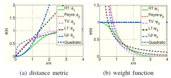
Comparison of the distance metrics ϕ and corresponding weight functions ϕ: The different distance metrics and the weight functions are plotted in (a) and (b), respectively. Note that the convex distance functions, shown by the blue and black curves, do not saturate with the Euclidean interpatch distances. In contrast, the distance functions corresponding to the current nonlocal schemes saturate as the patches become dissimilar. This ensures that the distances between dissimilar patches are not penalized, thus minimizing the blurring compared to the convex choices. This is also observed by the weights in the sum in (6). Note that the weights associated with the current schemes decay to zero for large distances. The slow decay of the weights associated with the convex metrics can result in blurred reconstructions. The l_p; p = 0.3 norms saturate rapidly, when compared to other non-local metrics, resulting in reduced averaging of similar patches.

Note that (18) involves the weighted norm of the patch differences. This expression is the sum of pixel differences:

$$\begin{array}{cc}\hfill g_{w_n}\left(f\right)& =\sum _{\mathrm{x}\in \Omega }\sum _{y\in N_{\mathrm{x}}}{w}_f\left(x,y\right)\underset{\sum _{\mathrm{p}\in B_{\mathrm{x}}}\eta \left(\mathrm{p}\right)\mid f(\mathrm{x}+\mathrm{p}-f\left(y+p\right)){\mid }^2}{\overset{\Vert P_{\mathrm{x}}\left(f\right)-P_{\mathrm{y}}\left(f\right){\Vert }_{\eta }^2}{\overbrace{}}}\hfill \\ \hfill & =\sum _{\mathrm{x}\in \Omega }\sum _{y\in N_{\mathrm{x}}}{\gamma }_f\left(x,y\right)\mid f\left(\mathrm{x}\right)-f\left(\mathrm{y}\right){\mid }^2\hfill \end{array}$$ (19)

We used a change of variables x = x + p and y = y + p and the symmetry of η(p) to derive the second step in (19). The weights γf are specified by

$${\gamma }_f\left(x,y\right)=\sum _{p\in B_{\mathrm{x}}}\eta \left(\mathrm{p}\right)w_f\left(x-p,y-p\right).$$ (20)

Note that the surrogate criterion G_w in (19) is similar to the H₁ NL penalty. The only difference is that the weights γf (x, y) are obtained as the sum of the similarity measures wf (x, y) between all the patch pairs that contain the pixels x and y (See Fig. 1.b). This summation is required to ensure that the algorithm is consistent with the minimization of the cost-function (12). We will now show the similarity of the current methods to the first iteration of the proposed scheme.

C. Similarity to current non-local methods

We now illustrate the similarity of current nonlocal regularization penalties to the surrogate functional G_w(f). Specifically, we choose the robust distance function ϕ(·) such that the expressions of G_w(f) and w_f (x, y) match the current schemes.

1) H1 nonlocal regularization

If the distance metric is chosen as

$$\varphi \left(z\right)=\left(1-\exp \left(-\frac{z^2}{{\sigma }^2}\right)\right),$$ (21)

we obtain $\psi \left(z\right)=\exp \left(-\frac{z^2}{{\sigma }^2}\right)∕{\sigma }^2$ using (16) Note that this choice of weights is very similar to the classical H₁ NL regularization. The main difference between the majorization and the H₁ scheme is that the weights in (19) are obtained as the summation of the similarity measures (see (20)). In contrast, the similarity measures themselves are used as weights in classical H₁ regularization. For convenience, we will refer to the metric in (21) as the H₁ distance function.

2) Peyre’s scheme

The NL penalty term (8) in Peyre’s NL method involves a weighted sum of l₁ norms of patch differences. Peyre’s scheme can also be expressed as a majorization of the proposed penalty by setting $\varphi \left(\upsilon \right)=\phi \left(\sqrt{\upsilon }\right)$ and using (11):

$$\phi \left(\sqrt{\Vert P_{\mathrm{x}}f-P_{\mathrm{y}}f\Vert }\right)\le \underset{\eta \left(x,y\right)}{\overset{\left(\frac{{\phi }^{\prime }\left(\sqrt{\Vert P_{\mathrm{x}}f-P_{\mathrm{y}}f\Vert }\right)}{2\sqrt{\Vert P_{\mathrm{x}}f-P_{\mathrm{y}}f\Vert }}\right)}{\underbrace{}}}\Vert P_{\mathrm{x}}f-P_{\mathrm{y}}f\Vert$$ (22)

Here, b is a constant that is safely ignored. The right hand side of the above expression is the same form as (8). From side of the above expression is the same form as (8). From the above expression, the weights are obtained as $\eta (\mathrm{x},\mathrm{y})=({\phi }^{\prime }\left(\upsilon \right)∕2\upsilon )$ where $\upsilon =\sqrt{\Vert P_{\mathrm{x}}f-P_{\mathrm{y}}f\Vert }$. Comparing with the expression of the weights used in Peyre’s scheme, specified by (0), we have $\frac{{\phi }^{\prime }\left(\upsilon \right)}{2\upsilon }=e^{-{\upsilon }^2}∕\sigma$. This equation is satisfied if $\phi \left(\upsilon \right)=\sigma \left(1-e^{-{\upsilon }^2∕\sigma }\right)$. Thus, the equivalent distance metric in (12) is given by

$$\varphi \left(x\right)=\phi \sqrt{x}=(1-e^{-x∕\sigma }).$$ (23)

We ignored the constant factor σ to ensure consistency between the different metrics. For convenience, we will refer to the metric in (23) as Peyre's distance function in the rest of the paper.

3) Nonlocal TV (NLTV) scheme

The nonlocal TV penalty in (7) involves the weighted l₁ norm of pixel differences. Since the l₁ norm of differences between two patches cannot be expressed as the sum of l₁ norms of the corresponding pixel differences, the NLTV scheme cannot be expressed as a special case of the proposed framework. However, if the penalty involves the l₁ norm of the patch differences as in (8), the corresponding NL scheme can be viewed as the majorization of the proposed scheme. Proceeding as in the Peyre’s case, we have $\frac{{\phi }^{\prime }\left(\sqrt{\upsilon }\right)}{2\sqrt{\upsilon }}=e^{-{\upsilon }^2∕{\sigma }^2}$. If we set $\varphi \left(\upsilon \right)=\phi \left(\sqrt{\upsilon }\right)$ we have ${\phi }^{\prime }\left(\upsilon \right)=\frac{{\phi }^{\prime }\left(\sqrt{\upsilon }\right)}{2\sqrt{\upsilon }}=e^{-{\upsilon }^2∕{\sigma }^2}$. This relationship is satisfied when the distance metric is specified by

$$\varphi \left(x\right)=\mathrm{erf}\left(\frac{x}{\sigma }\right)$$ (24)

For convenience, we will refer to the metric in (24) as NL TV distance function in the rest of the paper.

4) Convex nonlocal regularization

All of the above distance metrics are non-convex. Hence, the corresponding algorithms are not guaranteed to converge to the global minimum. The distance function can be chosen as a convex function to overcome this problem [17]:

$$\varphi \left(x\right)=\frac{\mid x\mid }{\sigma 1}.$$ (25)

Our experiments show that use of such convex cost functions result in blurring at high acceleration factors, compared to the non-convex choices considered above.

We list the current NL schemes, which are specified by the regularization functional J_w and the specific formula to compute the weights, in Table 1. We re-interpret these methods as the first iteration of a MM scheme to solve for the minimum of (12). The corresponding penalty functions ϕ are also shown in Table 1. We also show in next section that the proposed criterion can be efficiently minimized using MM algorithms, which rely on the re-computation of weights using ψ; the expressions for ψ is also listed in Table 1. The ϕ and the ψ functions are plotted in Fig. 2. We also plot the quadratic penalty $\varphi \left(x\right)=\mid x{\mid }^2$ and the corresponding weights for comparison. It is seen that the quadratic choice encourages the averaging of all patches in the neighborhood. In contrast, the equivalent ϕ functions of current nonlocal schemes H₁, TV, and Peyre's scheme) saturate with increasing inter-patch distance. This behaviour discourages the averaging of dissimilar patches, thus minimizing the blurring, compared to quadratic schemes that encourage uniform smoothing. Note that the above metrics saturate faster than the convex l₁ metric, thus providing reduced blurring. Note that this case is very different from convex local smoothness regularization, where the penalty only involves distances a pixel and its immediate neighbors. Since the NL penalty involves the distances between each patch and several other patches, this penalty can result in significant blurring if the functional does not saturate with the Euclidean distance.

TABLE I.

Reinterpretation of current nonlocal schemes

Current methods		Re-interpretation
Reference	Current algorithm Jw(f) and w(x, y)	Penalty function ϕ(x)	Weight function ψ(x)
H1 [11], [14]	(6) and (2)	(l − exp (− x2/2σ2))	exp (−x2/2σ2)
Peyre et al., [15]	(8) and (9)	(1 − e − x/σ)	$\frac{\exp (-x∕\sigma )}{2\sigma x}$
nonlocal TV [11], [12]	(7) and (2)	$\mathrm{erf}\left(\frac{x}{\sigma }\right)$	$\frac{\exp (-x^2∕{\sigma }^2)}{\sqrt{\pi }\sigma x}$
nonlocal L1 [17]	-	$\frac{x}{\sigma }$	$\frac{1}{2\sigma x}$

IV. Numerical algorithm

In the previous section, we used the majorization of the penalty term in (12) to illustrate the similarity of the proposed scheme to current NL methods. We now realize efficient algorithms based on alternate majorizations of (12). Since the penalty term is majorized in Section III-B, we term the resulting scheme as a penalty majorization (PM) algorithm. We also consider algorithms based on the majorization of the data consistency term (denoted by DM), and majorization of both data consistency and penalty terms (denoted by DPM). Thanks to the unified treatment, all of these algorithms can be used with any distance function ϕ This is an advantage over current schemes, which develop customized algorithms for each specific choice of J_w and ψ [11], [14], [15].

A. Majorization of the penalty term (PM)

We use the majorization of the regularization penalty, introduced in Section III-B, to develop a two-step alternating algorithm. The algorithm alternates between the solution of the quadratic surrogate problem:

$${\widehat{f}}_{n+1}=\underset{c_{n+1}}{\overset{\arg \underset{f}{\min }\Vert \mathrm{Af}-\mathrm{b}{\Vert }_2^2+\lambda \underset{{\mathrm{f}}^T{\Gamma }_n\mathrm{f}}{\overset{g_w\left(f\right)}{\overbrace{}}}}{\underbrace{}}}.$$ (26)

and the estimation of the weights form the current iterate as ${\mathrm{w}}_{f_n}(\mathrm{x},\mathrm{y})=\psi (\Vert P_{\mathrm{x}}\left(f_n\right)-P_{\mathrm{y}}\left(f_n\right){\Vert }_{\eta })$. Here, f is the vectorized image, A is the matrix operator corresponding to the forward model, and Γ_n is the sparse matrix with the entries: ${\Gamma }_n(\mathrm{x},\mathrm{y})={\gamma }_{f_n}(\mathrm{x},\mathrm{y})$. Here, γ f_n (x, y) is the sum of similarity measures w (x, y) using (20). This approach is inspired by the iterative reweighted least squares (IRLS) methods widely used in total variation and l₁ minimization schemes [26]. Note that the optimization criterion is a quadratic. The gradient of this criterion is obtained as

$$\nabla C_{n+1}=2({\mathrm{A}}^T\left(\mathrm{Af}-b\right)+\lambda {\Gamma }_n\mathrm{f}).$$ (27)

We propose to minimize the sub-criteria C_n+1 (f) using conjugate gradients algorithm (CG). We observe the CG algorithm provides significantly faster convergence compared to the steepest descent scheme used in [13] to solve (26). The CG scheme may be further accelerated using efficient preconditioning steps.

This two-step alternating scheme is similar to iterating the classical H₁ NL algorithm, followed by the re-estimation of the weights from the current image iterate. However, the interpretation of this approach as a specific algorithm to solve the global optimization problem (12) provides useful insights on the alternating strategy. For example, it enables us to monitor whether the algorithm is trapped in local minima and device continuation strategies to overcome such problems. This reinterpretation may also enable the development of novel algorithms to directly minimize (12). Moreover, since the different NL regularization penalties (NL TV, l₁ and Peyre’s schemes) can be interpreted as a special case of the global penalty, the same algorithms can be used for a range of NL penalties.

B. Majorization of the data term (DM)

The data majorization approach was originally introduced by Combettes et al., [27] for l₁ regularized problems. The main idea is to majorize the data term in (12) as

$$\Vert \mathrm{Af}-b{\Vert }^2\le \tau \Vert \mathrm{f}-{\mathrm{z}}_n{\Vert }^2,$$ (28)

where

$${\mathrm{z}}_n={\mathrm{f}}_n-{\mathrm{A}}^T({\mathrm{Af}}_n-\mathrm{b})$$ (29)

and $\tau \mathrm{I}\le A^{T}A$ for an appropriately chosen Γ. For example, when A is the one dimensional Cartesian Fourier undersampling operator, we have $\tau =\frac{M}{N}$ where M is the number of the samples that are retained and N is the length of the signal. Using this majorization, we obtain the surrogate criterion of 12) at the n^th iteration as

$$C_n\left(f\right)=\Vert f-z_n{\Vert }^2+\frac{\lambda }{\tau }g\left(f\right)$$ (30)

The minimization of C_n(f) is essentially a denoising problem, which can be solved using the fixed point iterative algorithm 21]. Specifically, the Euler-Lagrange equation of the above criterion is given by

$$z_n-f=\frac{\lambda }{2\tau }\sum _{\mathrm{y}\in N_{\mathrm{x}}}\underset{w_f(\mathrm{x},\mathrm{y})=\psi (\Vert P_{\mathrm{x}}\left(f\right)-P_{\mathrm{y}}\left(f\right){\Vert }_{\eta })}{\overset{\frac{{\varphi }^{\prime }({\Vert }_{\mathrm{x}}\left(f\right)-P_{\mathrm{y}}\left(f\right){\Vert }_{\eta })}{\Vert P_{\mathrm{x}}\left(f\right)-P_{\mathrm{y}}\left(f\right){\Vert }_{\eta }}}{\underbrace{}}}{(P_{\mathrm{x}}\left(f\right)-P_{\mathrm{y}}\left(f\right))}_{\eta }$$ (31)

This equation can be rewritten in terms of pixel differences as

$$f\left(\mathrm{x}\right)-z_n\left(\mathrm{x}\right)+\frac{\lambda }{2\tau }\sum _{y\in N_{\mathrm{x}}}{\nu }_f\left(x,y\right)(f\left(\mathrm{x}\right)-f\left(\mathrm{y}\right))=0,$$ (32)

where νf_n is defined as in (20). Thus, the solution to (30) can be obtained using the following fixed point iterations [21]

$$f_{n,m+1}\left(\mathrm{x}\right)=\frac{z_n\left(\mathrm{x}\right)+\frac{\lambda }{2\tau }{\Sigma }_{\mathrm{y}\in N_{\mathrm{x}}}{\nu }_{f_{n,m}}(\mathrm{x},\mathrm{y})f_{n,m}\left(\mathrm{y}\right)}{1+\frac{\lambda }{2\tau }{\Sigma }_{\mathrm{y}\in N_{\mathrm{x}}}{\nu }_{f_{n,m}}(\mathrm{x},\mathrm{y})}.$$ (33)

Here, m is the index for the inner loop. Thus, the each step of the algorithm involves one steepest descent step (29), followed by nonlocal denoising using several fixed point iterations. Note that each iteration of the fixed point algorithm requires the re-estimation of the weights νf_{n, m}, which is computationally expensive.

C. Majorization of both the data and penalty terms (DPM)

Following the data majorization in (30), we now additonally majorize the penalty term to obtain

$$D_n\left(f\right)=\Vert f-z_n{\Vert }^2+\frac{\lambda }{\tau }\sum _{\mathrm{x}\in \Omega }\sum _{y\in N_{\mathrm{x}}}{\nu }_{f_n}(\mathrm{x},\mathrm{y})\Vert f\left(\mathrm{x}\right)-f\left(\mathrm{y}\right){\Vert }^2$$ (34)

Solving this criterion as before, we get

$$f_{n+1}\left(\mathrm{x}\right)=\frac{z_n\left(\mathrm{x}\right)+\frac{\lambda }{2\tau }{\Sigma }_{\mathrm{y}\in N_{\mathrm{x}}}{\nu }_{f_n}(\mathrm{x},\mathrm{y})f\left(\mathrm{y}\right)}{1+\frac{\lambda }{2\tau }{\Sigma }_{\mathrm{y}\in N_{\mathrm{x}}}{\nu }_{f_n}(\mathrm{x},\mathrm{y})}.$$ (35)

This equation is similar to (33), except that only one fixed point update is required at each iteration. Thus, this algorithm alternates between one steepest-descent step and one fixed point step. As in the DM case, the weights have to be reestimated for each steepest descent step. This approach is similar to the algorithms used in [17] and [16].

D. Summary of the MM algorithms

Each iteration of the above four algorithms involves the following steps:

• PM-CG: One weight update, followed by iterative CG optimization, until convergence; this algorithm is introduced in this paper.

• PM-SD: One weight update, followed by several steepest descent updates; this is the approach followed in [13] to solve conventional NL regularization problems.

• DM: One steepest descent update, followed by several fixed point steps (each involving one weight evaluation). The fixed point iteration to solve denoising problems is introduced in [21].

• PDM One steepest descent update, followed by one fixed point step (each fixed point step involving one weight evaluation); this is the approach followed in [17].

The computation of the weights w_f (x, y) involves the evaluation of the distances between all patch pairs (see (16) and hence is computationally expensive. In contrast, each of the CG steps involves three FFTs (in Fourier inversion and deblurring applications) and a weighted linear combination of pixel values (evaluation of Γ _n f per iteration; these steps are relatively inexpensive compared to the evaluation of the weights. Since the PM-CG scheme relies on one weight computation, followed by several CG updates, we expect this algorithm to be more efficient than other methods. Note that the MD and MPD schemes require at least one weight computation per one steepest descent step.

E. Expression of the weights for specific distance metrics

All of the above algorithms require the repeated evaluation of ν_fn (x, y), which are computed from the similarity measures $w_n(\mathrm{x},\mathrm{y})=\psi (\Vert P_{\mathrm{x}}\left(f\right)-P_{\mathrm{x}}\left(f\right){\Vert }_{\eta })$ using (20). We focus on the specific distance function (ϕ) considered earlier and derive the expression for the corresponding ψ functions.

1) H1 distance metric

Applying (16) to the distance metric ϕ specified by (21), we obtain

$$\psi \left(x\right)=\frac{{\varphi }^{\prime }\left(x\right)}{x}=\frac{1}{{\sigma }^2}\exp (-x^2∕{\sigma }^2).$$

This Gaussian weight function is widely used in nonlocal H₁ algorithms.

2) Peyre’s distance metric

When ϕ(x) is specified by (23), we obtain

$$\psi \left(x\right)=\frac{\exp (-x∕\sigma )}{2\sigma x}.$$

The iterative reweighted quadratic minimization scheme is considerably simpler than the current non-linear minimization schemes used for nonlocal TV [11].

4) l₁ distance metric

In the l₁ case, we obtain

$$\psi \left(x\right)=\frac{\exp (-x^2∕{\sigma }^2)}{\sqrt{\pi }\sigma x}.$$

We plot the four ψ functions in Fig. 2(b), along with ψ(x) = 1, which corresponds to ϕ(x) = x². Note that this choice results in the averaging of all the patches in the specified neighborhood, irrespective of the similarity. In contrast, the weights corresponding to other NL penalties decay with Euclidean inter-patch distances, ensuring that dissimilar patches are not averaged. The smoothing properties are determined by the rate of decay of ψ. For example, the slow decay of the the weight function corresponding to the convex l₁ metric results in blurred reconstructions. In contrast, the weights corresponding to the non-convex distances decay rapidly, resulting in less blurred reconstructions. This explains the desirable properties of the non-convex distance measures, which are also confirmed by our experimental results.

F. Continuation to improve convergence to global minimum

Since non-convex distance functions have narrow valleys, they discourage the averaging of dissimilar patches, while promoting the averaging of similar patches, resulting in improved reconstructions. However, the main challenge associated with non-convex distance metrics is the convergence of the alternating algorithm to the local minima of (12). To improve the convergence to the global minimum, we propose to use a continuation strategy.

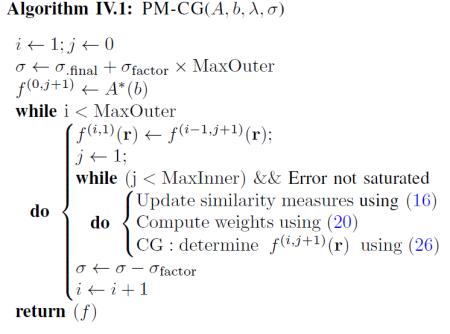
Note from Fig.8 that the non-convex distance functions closely approximate quadratic or convex l₁ functions when x/σ << 1. The distance functions saturate only when x/σ > 1. We use this property to realize the continuation scheme. Specifically, we start with large values of σ and reduce it to the desired value in several steps. At each step, we use the image iterate corresponding to the σ value at the previous iteration as the initialization. This approach is similar to the homotopy continuation scheme used in non-convex compressive sensing 28], which were reported to be very effective. We initialize the algorithm with σ_final + σ_incfactor × MaxOuter. We decrement σ by σ_incfactor at each outer iteration. Thus, in the final iteration, we algorithm uses σ = σ_final. In this work, we choose σincfactor = 5. The pseudo-code of the proposed PMCG scheme with continuation is shown below.

Fig. 8.

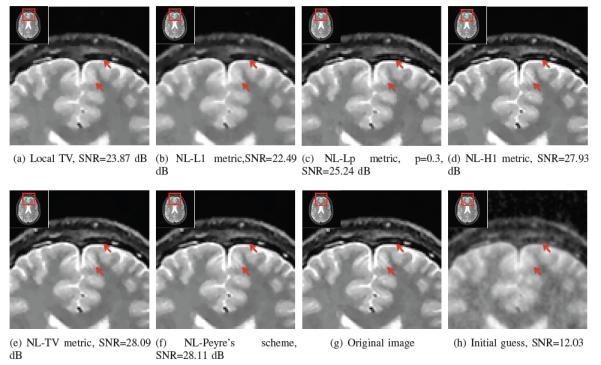
Comparison of the proposed algorithm with different metrics against classical schemes: We reconstruct the 256 × 256 MRI brain image from its sparse Fourier samples. We consider an under sampling factor of 4. We choose the standard deviation of the complex noise that is added to the measurements such that the SNR of the measurements is 40dB. We observe that the proposed schemes that use non-convex distance metrics provide the best SNR, which is around 4.22 dB better than local TV. The use of convex distance metrics can only provide reconstructions than are comparable to local TV. The l_p; p = 0.3 penalty provides improved results than the p = 1 case. However, the performance improvement is not as significant as the other non-local metrics, probably due to the reduced averaging of similar patches. The arrows indicate the details preserved by the non-convex schemes, but missed by local TV and convex non-local algorithm.

V. Experimental results

We introduced a unifying non-local regularization framework, where the regularization penalty is the unweighted sum of robust distances between image patch pairs. In addition to providing a justification for the heuristic approach of iterating current NL algorithms, the novel framework enabled us to understand and mitigate the alias amplification issues that are widely reported in the context of Fourier inversion. In this section, we will determine the utility of the continuation scheme, introduced in Section IV-F, to overcome the local minima problems. The similarity of the proposed framework with regularization schemes in compressive sensing enabled us to develop computationally efficient algorithms. We compare the computational efficiency of the proposed algorithms in this section. Thanks to the unifying framework, these fast methods are applicable to a wide range of NL penalties. We also study the impact of the various parameters and distance metrics on image quality, and compare the non-local schemes with local TV algorithms.

A. Utility of continuation

We aim to recover a 128×128 Shepp Logan phantom from ten lines and a 256×256 brain image from its five fold under sampled measurements in the Fourier domain. We used the nonlocal H1 and TV distance functions. We assume that the measurements are corrupted by complex Gaussian noise, such that the SNR of the noise k-space data is 50dB. The original images are shown in Fig. 4.(a) and Fig. 4.(f), while the initial guesses obtained by computing zero filled inverse Fourier transform are shown in Fig. 4.(b) and Fig. 4.(g), respectively. The heuristic alternating algorithm results in reconstructions with amplified alias artifacts (see (c) and h)). We observe that the continuation strategy, illustrated in Fig. 3.(a) & (b), is capable of removing the alias artifacts completely. This convergence can also be appreciated by the plot of the cost in Fig. 4.(e). It is seen that the cost function saturate to high values (red dotted and solid lines) because the algorithms get stuck in local minima of (12), when no continuation is used. In contrast, they converge to smaller costs with the continuation scheme. We confirmed that this is indeed the global minimum of the criterion by using multiple initializations, including the original image. The improved performance can also be appreciated by the SNR plots shown in Fig. 4.(j). This experiment shows that non-convex metrics can provide improved reconstructions in challenging inverse problems, but continuation schemes are essential to minimize the convergence to local minima.

Fig. 4.

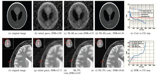
Utility of continuation: We consider the recovery of a 128x128 Shepp Logan phantom from its ten radial lines in the Fourier domain in (a)-(d). The classical alternating algorithm emphasizes the alias artifacts in the initial guess in (b), which is obtained by zero-filled IFFT. Specifically, the result in (c) correspond to a local minimum of (12). The use of the continuation scheme mitigated these issues as seen in (d). We also consider the reconstruction of a 256 × 256 MRI brain image from 46 uniformly spaced radial lines in the Fourier domain. We observe that the alternating algorithm results in the enhancement of the alias artifacts (see (h)). These problems are eliminated by the continuation scheme, shown in (i). The behavior of the algorithms can be better understood from the cost vs iterations shown in (e). It is observed that the continuation schemes shown in blue solid and dotted lines (corresponding to Shepp-Logan and brain images, respectively) converge to a lower minimum than the methods without continuation (red solid and dotted lines). The improvement in performance is also SNR vs CG step plot in (j).

Fig. 3.

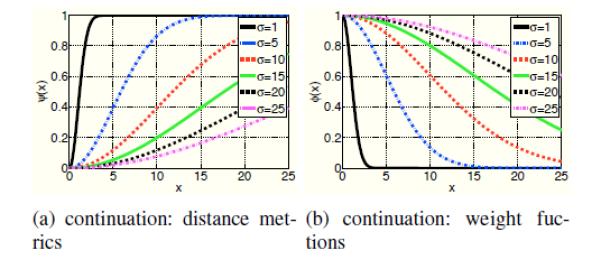
Illustration of the continuation scheme used to minimize the convergence of the algorithm to local minimum. We start with σ = 25, when the distance metric is convex for most patch pairs in the image. We then gradually reduce the value of σ by a step size of 5 until it achieves the desired value σ = 1. Note that the distance metrics with small values of σ are non-convex.

B. Utility of iterating between weight and image estimation

Since alternating schemes result in alias amplification in the context of Fourier inversion, current NL schemes use fixed weights with such challenging problems. The weights are often estimated from the noisy/smoothed image [13], [15], [29] and Tikhonov or total variation regularized reconstructions in deblurring applications [13]. We demonstrate the improvement offered by the proposed scheme with continuation, compared to these fixed weight methods in Fig.5. We consider the recovery of a brain MRI image from five fold randomly under-sampled Fourier data. We consider three different fixed weights, which are estimated from different initial estimates: a) zero padded inverse Fourier transform A^* of the measurements, b) Tikhonov regularized reconstruction, and (c) local TV regularized reconstruction. We initialize the PM-CG scheme with weights obtained from zero-padded IFFT reconstruction. We observe that the the iterative strategy provides a 4 dB improvement over the best fixed weight scheme. These experiments demonstrate that the quality of the reconstructions can be significantly improved by the iterative framework with appropriate continuation strategies to ensure convergence to global minima.

Fig. 5.

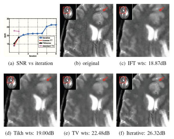
Comparison of current algorithms with pre-computed weights and the proposed iterative framework: We consider the reconstruction of the MRI brain image from 20% of its random Fourier samples using the H₁ distance metric. In Fig. 5(a), we plot the improvement in signal to noise ratio as a function of the number of iterations. The zeroth iteration correspond to the different initial guesses. These guesses are derived with three different algorithms: zero filled inverse FFT (red), Tikhonov reconstruction (black), and local TV (majenta). Since the current NL schemes do not re-estimate the weights, only one iteration is involved. The blue curve corresponds to the proposed iterative scheme, which re-estimates the weights from the current image estimate. Since this scheme is also initialized with the zero filled IFFT, the red and the blue curves overlap. Note that the proposed iterative method provides significantly improved reconstructions.

C. Comparison of optimization algorithms

We compare the convergence rate and computation complexity of the four MM algorithms, described in Section IV, in Fig. 6. Here, we consider the reconstruction of a 128 × 128 Shepp-Logan phantom from 16 radial lines in the Fourier domain/k-space. We choose ϕ as the H₁ distance metric, specified by (21). We set λ = 50 and σ = 10, since this choice of parameters gives the best reconstruction. Note that the PM-CG scheme requires around 20 times fewer CG steps to converge, compared with other algorithms. In addition, the computational complexity of each iteration of the PM scheme is lower than DM and DPM methods, since the computationally expensive weight computations are performed only in the outer loop. In this specific example, the PM-CG scheme requires around 33 seconds to converge, while the DM and PDM algorithms require 5000 seconds or more. The experiments are performed on a laptop with 2.4 GHz Duo Core CPU processor and 4 GB memory in MATLAB R2010a. Since the PM-CG scheme is significantly more computationally efficient than other methods, we will use this method for all the other experiments considered in this paper. Thanks to the unification offered by the proposed scheme, we can now use this algorithm for all the distance metrics.

Fig. 6.

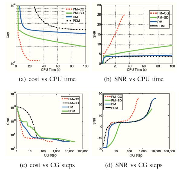
Comparison of optimization algorithms: We focus on the recovery of a 128 × 128 Shepp-Logan phantom from 16 radial lines in the Fourier domain by minimizing (12). The decay of the cost function (12) as a function of the number of conjugate gradient steps (inner iterations) and CPU time are shown in (a) and (b), respectively. The improvement in SNR as a function of iterations and CPU time are shown in (c) and (d), respectively. Note that all the optimization algorithms converge to the same minima. However, the PMCG scheme requires much fewer (20 fold) number of iterations. Moreover, the computational complexity per iteration of this method is also lower since the expensive weight computation is only performed in the outer loop.

D. Choice of parameters

There are various parameters in the proposed nonlocal algorithms, such as regularization parameter λ size of the search window N_x and patch size P_x. We now study the effect of these parameters on the quality of the reconstructions. The parameter λ controls the trade off between data fidelity and regularization. To ensure fair comparisons, we search the optimal λ for each algorithm, measurement, and noise level. We pick the value of λ that provides the best reconstruction in each case. To keep the computational complexity manageable, most NL schemes do not search the entire image for similar patches.

We study the effect of patch size N_p and neighborhood size N_w in the context of image denoising² in Fig.7. We add Gaussian noise to the Shepp-Logan phantom such that the SNR of the noisy image is 16dB. We then use nonlocal H1 and TV penalties to recover the image. The results are shown in Fig. 7. We observe that the performance of the algorithms degrade with increasing patch size. This is expected since increasing the size of the patches will result in decreased number of patches similar to it. The more interesting observation is that increasing the size of the neighborhood results in decreased SNR with only one exception. Specifically, the SNR improves slightly while the neighborhood size is increased from N_w = 5 to N_w = 7 in NL TV with patch size N_w = 3. These findings can be explained using the unified formulation. Note that the metric in (13) involves the unweighted sum of distances between all patch pairs in the neighborhood. As we increase N_w we compare more dissimilar patches. If the distance function ϕ (x) does not saturate to one with large values of x, the functional in (13) will continue to penalize the distances between dissimilar patches and hence result in blurring. Note that the TV penalty saturates much faster than the H₁ penalty, which explains the improvement in performance when N_w is increased from 5 to 7. The comparisons in Fig.7 show that choosing N_p × N_p = 3 × 3 and N_w × N_w = 5 × 5 are sufficient to obtain good results. Even though the results may change slightly depending on the image and the type of application, we will use these parameters in the rest of the paper.

Fig. 7.

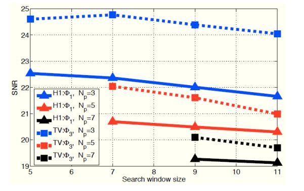
Impact of the parameters on reconstruction accuracy: We consider the denoising of noisy Shepp-Logan phantom image with a SNR of 16 dB. We plot the change in the SNR of the denoised image as a function of the search window size N_w. The blue, red, and black curves correspond to N_p = 3, N_p = 5, and N_p = 7, respectively. The plot shows that SNR of the images degrades with increasing N_p. This is expected since the number of similar patches decrease with increasing patch size. We observe that the SNR also decreases with increasing window size, except for the non-local TV distance metric with N_w = 7. See text for more explanation.

The reason for obtaining good reconstructions with smaller search window sizes is due to the ability of iterative NL schemes to exploit the similarities between patch pairs, even when they are not in each others neighborhood. It is sufficient that they are linked by at least one similar patch that is in both the neighborhoods. i.e, if P_x (f) ≈ P_y (f) ≈ P_z (f) and y ∊ N_x and y ∊ N_z, then the algorithm can exploit the similarity between P_x (f) and P_z (f), even when z ∉ N_x. This is enabled by the terms $\varphi (\Vert P_x\left(f\right)-P_y\left(f\right)\Vert )$ and $\varphi (\Vert P_r\left(f\right)-P_z\left(f\right)\Vert )$ in the proposed NL penalty. Since conventional NL means smoothing filters are non-iterative, they are not capable of exploiting the similarity between patches that are not in each others neighborhoods.

E. Image reconstruction with different distance metrics

We compare the proposed NL scheme with different nonlocal distance metrics (see Table I), in the context of image recovery from sparse Fourier samples. We use popular test images (e.g., Lena and cameraman) as well as multiple typical MRI images (e.g., brain and cardiac MRI images). We also compare the non-local schemes against local TV and wavelet algorithms to bench mark the performance. The comparisons of the methods on a MRI brain image is shown in Fig. 8. Here we consider a downsampling factor of 4 and the downsampling pattern is random with non-uniform k-space density. We add complex Gaussian white noise to the measured data such that the SNR of measurements is 40dB. Continuation schemes are used with non-convex non-local methods to minimize the local minima effects. We observe that the non-convex algorithms provide the best reconstructions. In contrast, the proposed nonlocal scheme with the L₁ metric results in reconstructions with significant blurring, while the local TV scheme provides patchy reconstructions. The nonlocal TV metric gives the highest SNR, followed by nonlocal H1. A similar comparison is performed in Fig. 9, where we recover another MRI brain image with a tumor from its five fold under-sampled Fourier data set. We use the polar trajectory with 52 radial lines to sample. Gaussian noise is added to the k-space data such that the noise level of the measurements is 80dB. The zoomed versions of different regions of the image is shown in Fig. 9. We observe that proposed NL method using the non-convex metrics (TV, H1, and Peyre’s schemes) provides better results than the local TV scheme, and non-local scheme using the L1 metric results.

Fig. 9.

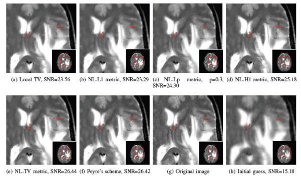
Comparison of the proposed algorithm with different metrics against classical schemes: We reconstruct the 256 × 256 MRI brain image from its sparse Fourier samples. We consider an under sampling factor of 5. We choose the standard deviation of the gaussian noise that is added to the measurements such that the SNR of the measurements is 40dB. We observe that the proposed schemes that use non-convex distance metrics provide the best SNR, which is around 3 dB better than local TV. The arrows indicate the details preserved by the non-convex schemes, but missed by local TV and convex non-local algorithm.

The signal to noise ratios of the reconstructions of different images using the different algorithms are shown in Table II. We consider an acceleration of 5 and the Fourier space is sampled randomly using a non-uniform k-space density. We observe that the proposed nonlocal algorithm with non-convex penalties consistently outperform the local TV algorithm, resulting in an improvement of more than 2-3 dB. In contrast, the SNR of the non-local scheme with convex l₁ distance metric is only comparable to the local TV scheme.

TABLE II.

Signal to noise ratio of the reconstructed images using different algorithms.

Image	local TV	nonlocal L1	H1 metrix	NLTV metric	Peyre’s metric
lena	20.46	20.97	23.37	23.93	24.05
cameraman	23.31	23.04	24.84	25.88	25.99
brain1	23.24	22.48	26.12	27.51	27.45
brain2	22.24	22.12	27.15	28.06	27.99
ankle	21.41	22.23	23.43	24.56	24.70
abdomen	16.45	16.90	18.51	19.46	19.70
heart	20.32	21.56	22.26	24.47	24.90

VI. Conclusion

We introduced a unifying energy minimization framework for the nonlocal regularization of inverse problems. The proposed functional is the unweighted sum of inter-patch distances. We showed that the first iteration of a MM algorithm to minimize the proposed cost function is similar to the classical non-local means algorithms. Thus, the reformulation provided a theoretical justification for the heuristic approach of iterating non-local schemes, which re-estimate the weights from the current image estimate. Thanks to the reformulation, we now understand that the widely reported alias enhancement issues with iterative non-local methods are caused by the convergence of these algorithms to the local minimum of the proposed non-convex penalty. We introduce an efficient continuation strategy to overcome this problem. We introduced several fast majorize-minimize algorithms. Thanks to the unifying framework, all of the novel fast algorithms are readily applicable for a large class of non-local formulations.

References

- 1.Ma J, Dimet L. Deblurring from highly incomplete measurements for remote sensing. IEEE Trans. Geoscience and Remote Sensing. 2009;47(3):792–802. [Google Scholar]
- 2.Vogel C, Oman M. Fast, robust total variation-based reconstruction of noisy, blurredimages. IEEE Transactions on Image Processing. 1998 Jan; doi: 10.1109/83.679423. [DOI] [PubMed] [Google Scholar]
- 3.Osher S, Soleé A, Vese L. Image decomposition and restoration using total variation minimization and the h – 1 norm. Multiscale Modeling and Simulation. 2003;1:349–370. [Google Scholar]
- 4.Chambolle A, Lions PL. Image recovery via total variation minimization and related problems. Numerische Mathematik. 1997;76(2):167–188. [Google Scholar]
- 5.Lustig M, Donoho D, Pauly J. Sparse MRI: The application of compressed sensing for rapid MR imaging. MRM. 2007 Dec;58(6):1182–95. doi: 10.1002/mrm.21391. [DOI] [PubMed] [Google Scholar]
- 6.Vonesch C, Unser M. A fast multilevel algorithm for wavelet-regularized image restoration. IEEE Transactions on Image Processing. 2009;18(3):509–523. doi: 10.1109/TIP.2008.2008073. [DOI] [PubMed] [Google Scholar]
- 7.Guerquin-Kern M, Van De Ville D, C. Vonesch , J.C. Baritaux , Pruessmann KP, Unser M. Wavelet-regularized reconstruction for rapid MRI; ISBI 2007; 2009. pp. 193–196. IEEE. [Google Scholar]
- 8.Buades A, Coll B, Morel JM. A review of image denoising algorithms, with a new one. Multiscale Modeling and Simulation. 2006;4(2):490–530. [Google Scholar]
- 9.Awate SP, Whitaker RT. Unsupervised, information-theoretic, adaptive image filtering for image restoration. IEEE Trans. Pattern Recognition. 2006;28:364. doi: 10.1109/TPAMI.2006.64. [DOI] [PubMed] [Google Scholar]
- 10.Buades A, Coll B, Morel JM. Nonlocal image and movie denoising. International Journal of Computer Vision. 2008;76(2):123–139. [Google Scholar]
- 11.L.D. Cohen , Bougleux S, Peyreé G. Non-local regularization of inverse problems. European Conference on Computer Vision (ECCV’08) 2008 [Google Scholar]
- 12.Gilboa G, Darbon J, Osher S, Chan T. Nonlocal convex functionals for image regularization. UCLA CAM Report. 2006:06–57. [Google Scholar]
- 13.Lou Y, Zhang X, Osher S, Bertozzi A. Image recovery via nonlocal operators. Journal of Scientific Computing. 2010;42(2):185–197. [Google Scholar]
- 14.Zhang X, Burger M, Bresson X, Osher S. Bregmanized nonlocal regularization for deconvolution and sparse reconstruction. SIAM Journal on Imaging Sciences. 2010;3:253. [Google Scholar]
- 15.Peyreé G, Bougleux S, Cohen LD. Non-local regularization of inverse problems. Inverse Problems and Imaging. 2011:511–530. [Google Scholar]
- 16.Adluru G, Tasdizen T, Schabel MC, DiBella EVR. Reconstruction of 3D dynamic contrast-enhanced magnetic resonance imaging using nonlocal means. Journal of Magnetic Resonance Imaging. 2010;32(5):1217–1227. doi: 10.1002/jmri.22358. [DOI] [PubMed] [Google Scholar]
- 17.Wang G, Qi J. Patch-based regularization for iterative pet image reconstruction. IEEE ISBI. 2011 [Google Scholar]
- 18.Chartrand R. Exact reconstruction of sparse signals via nonconvex minimization. Signal Processing Letters. 2007;14(10):707–710. IEEE. [Google Scholar]
- 19.Figueiredo M, Dias J, Nowak R. Majorization-minimization algorithms for wavelet-based image restoration. IEEE Transactions on Image Processing. 2007;16(12):2980–2991. doi: 10.1109/tip.2007.909318. [DOI] [PubMed] [Google Scholar]
- 20.Yang J, Zhang Y. Alternating direction algorithms for ell1 problems in compressive sensing. Arxiv preprint arXiv:0912.1185. 2009 [Google Scholar]
- 21.Pizarro L, Mraézek P, Didas S, Grewenig S, Weickert J. Gener- alized nonlocal image smoothing. International Journal of Computer Vision. 2010;90:62–87. [Google Scholar]
- 22.Yang Z, Jacob M. A unified energy minimization framework for nonlocal regularization. IEEE ISBI. 2011 [Google Scholar]
- 23.Figueiredo M, Bioucas-Dias J, Oliveira J, Nowak R. On total variation denoising: A new majorization-minimization algorithm and an experimental comparison with wavalet denoising; IEEE International Conference on Image Processing.2006. p. 2633. [Google Scholar]
- 24.Figueiredo M, Dias J, Oliveira J, Nowak R. On total variation denoising: A new majorization-minimization algorithm and an experimental comparisonwith wavalet denoising; IEEE International Conference on Image Processing.2006. 2006. pp. 2633–2636. [Google Scholar]
- 25.Charbonnier P, Blanc-Feéraud L, Aubert G, Barlaud M. Deter- ministic edge-preserving regularization in computed imaging. Image Processing, IEEE Transactions on. 1997;6(2):298–311. doi: 10.1109/83.551699. [DOI] [PubMed] [Google Scholar]
- 26.Chartrand R, Wotao Yin. Iteratively reweighted algorithms for compressive sensing. Acoustics, Speech and Signal Processing, 2008; ICASSP 2008. IEEE International Conference on; 2008. pp. 3869–3872. april 4 2008. [Google Scholar]
- 27.L. Combettes P, Wajs VR. Signal recovery by proximal forward- backward splitting. Multiscale Modeling. 4(4):1168–1200. [Google Scholar]
- 28.Trzasko J, Manduca A. Highly undersampled magnetic resonance image reconstruction via homotopic l0-minimization. Medical Imaging, IEEE Transactions on. 2009;28(1):106–121. doi: 10.1109/TMI.2008.927346. [DOI] [PubMed] [Google Scholar]
- 29.Gilboa G, Osher S. Nonlocal operators with applications to Image Processing. Multiscale Model. Simul. 2008;7(3):1005–1028. [Google Scholar]
- 30.Brox T, Kleinschmidt O, Cremers D. Efficient nonlocal means for denoising of textural patterns. IEEE Transactions on Image Processing. 2008 Jul;17(7):1083–1092. doi: 10.1109/TIP.2008.924281. [DOI] [PubMed] [Google Scholar]