Multivariate Granger causality: an estimation framework based on factorization of the spectral density matrix

Abstract

Granger causality is increasingly being applied to multi-electrode neurophysiological and functional imaging data to characterize directional interactions between neurons and brain regions. For a multivariate dataset, one might be interested in different subsets of the recorded neurons or brain regions. According to the current estimation framework, for each subset, one conducts a separate autoregressive model fitting process, introducing the potential for unwanted variability and uncertainty. In this paper, we propose a multivariate framework for estimating Granger causality. It is based on spectral density matrix factorization and offers the advantage that the estimation of such a matrix needs to be done only once for the entire multivariate dataset. For any subset of recorded data, Granger causality can be calculated through factorizing the appropriate submatrix of the overall spectral density matrix.

1. Introduction

Cognitive functions are achieved through cooperative neural processing. Multi-electrode recording and functional imaging are key technologies to enable us to study network mechanisms of cognition and their breakdown in disease. Analytically, cross correlation functions and ordinary coherence spectra remain the main statistics for assessing interactions among the monitored nodes of a neuronal network. As the hypotheses concerning the role of neural interactions in cognitive paradigms become more elaborate, it is felt that being able to evaluate the direction of neural interactions in neural networks holds the key to teasing out the functional significance of different nodes in these networks. Recently, there has been considerable interest in a class of techniques called Granger causality to provide a statistically principled way to measure directional influences [1–20].

Typically, Granger causality is inferred parametrically through autoregressive models of time-series data. For a multivariate dataset recorded from a set of brain areas or neuronal ensembles, depending on the problem, one might be interested in different subsets of the recorded areas. According to the current estimation framework, for each subset, one conducts a separate model fitting process. Such an approach may introduce unwanted variability and uncertainty as the model parameters (e.g. model order) are often different for different subsets of data channels. In addition, our past work [16] has shown that Geweke's method for conditional Granger causality estimation, while theoretically sound, can give erroneous results in practice, because quantities assumed to be the same in different autoregressive models are not always the same when finite datasets and inevitable estimation errors are taken into account.

The goal of this paper is to provide a multivariate framework for estimating Granger causality that overcomes these shortcomings. We begin by reviewing the essential ideas of Granger causality with special emphasis on its spectral representation. The current estimation framework is then extended to a multivariate formalism based on the technique of spectral density matrix factorization. Numerical examples and experimental data are included to illustrate the theoretical ideas.

2. Material and methods

(a). Pairwise analysis

Consider two simultaneously recorded stationary time series. According to Wiener [21], if the prediction of one time series is improved by incorporating the knowledge of a second one, then the second series is said to have a causal influence on the first. Wiener's proposal lacks the machinery for practical implementation. Granger later formalized the prediction idea in the context of linear regression models [22]. Specifically, if the variance of the autoregressive prediction error of the first time series at the present time is reduced by inclusion of past measurements from the second time series, then the second time series is said to have a causal influence on the first one. Reversing the role of the two time series, one can consider the causal influence in the opposite direction. The interaction discovered this way could be either reciprocal or unidirectional. Below we first give a brief introduction to the mathematical formulation of Granger causality based on the more detailed exposition in [2], and then proceed to define the multivariate estimation framework.

Let the two stationary time series be denoted by X_t and Y _t. Individually, X_t and Y _t can each be represented by the following autoregressive models:

2.1

and

2.2

Jointly, they are represented as the following bivariate autoregressive model:

2.3

where ε_2t and η_2t are uncorrelated over time, and their contemporaneous covariance matrix is

2.4

The total interdependence between X_t and Y _t can be computed as

2.5

where |⋅| denotes the determinant of the enclosed matrix. When X_t and Y _t are independent, F_X,Y=0. When this total interdependence is non-zero, Geweke [23] showed that F_X,Y can be decomposed into three components,

2.6

where

2.7

and

2.8

are the linear causality from Y _t to X_t and from X_t to Y _t due to their interactions, and

2.9

is the instantaneous causality due to possibly common input exogenous to the bivariate time-series system X_t and Y _t.

After Fourier transforming the bivariate autoregressive representation (2.3) and applying proper ensemble average, we get the spectral density matrix

2.10

where the asterisk (*) denotes the complex conjugate and matrix transpose, and H(ω) is the transfer function matrix.

The spectral density matrix S(ω) contains cross-spectra (off-diagonal elements) and auto-spectra (diagonal elements). If X_t and Y _t are independent, then the cross-spectra are zero and the determinant |S(ω)| equals the product of two auto-spectra. This observation motivates the spectral domain representation of total interdependence between X_t and Y _t as

2.11

It is easy to see that this representation of interdependence is related to coherence by the following relation:

2.12

where the coherence function is defined as C(ω)=|S_xy(ω)|²/S_xx(ω)S_yy(ω).

Geweke [23] proved that the two directional measures can be computed explicitly according to

2.13

and

2.14

where and .

By defining the instantaneous causality spectra as

2.15

we achieve a decomposition of the total interdependence in the spectral domain that is analogous to equation (2.6) in the time domain, namely,

2.16

It is worth noting that the spectral instantaneous causality could become negative for some frequencies in certain situations and may not have a readily interpretable physical meaning on a frequency-by-frequency basis.

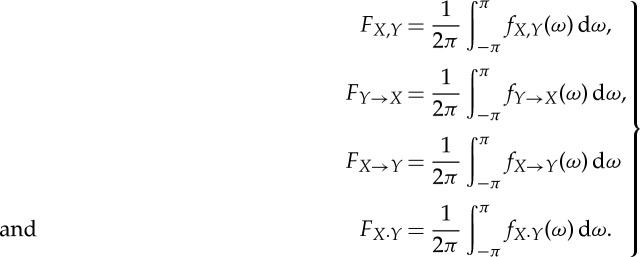
Under general conditions, the spectral measures integrated over the frequency yield their time-domain counterparts [23],

2.17

It is expected that the conditions necessary for these equalities to hold are met in practical applications.

(b). Conditional Granger causality

When there are three or more time series, a pairwise analysis can be performed using the above bivariate approach. Such a pairwise approach may lead to ambiguous results in terms of differentiating direct from mediated causal influences [2,16,24]. A conditional Granger causality analysis can help resolve the ambiguity. Consider three time series X_t, Y _t and Z_t. Suppose that a pairwise analysis reveals a causal influence from Y _t to X_t. The following procedure determines whether this influence has a direct component or is mediated entirely by Z_t.

Let the joint autoregressive representation of series X_t and Z_t be

2.18

where the covariance matrix of the noise vector is . Next, consider the joint autoregressive representation of all three time series X_t, Y _t and Z_t,

2.19

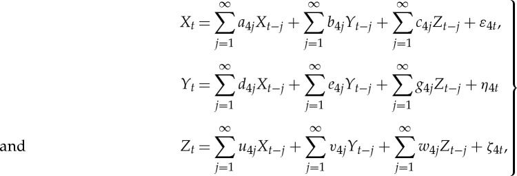
where the covariance matrix of the noise vector is . From these two sets of equations (2.18) and (2.19), the Granger causality from Y _t to X_t conditional on Z_t is defined as

2.20

If F_{Y →X|Z}>0 in some suitable statistical sense, then the inclusion of Y _t results in improved prediction of X_t, indicating that Y _t→X_t has a direct component. In contrast, if F_{Y →X|Z}=0, the influence Y _t→X_t is said to be entirely mediated by Z_t. Conditional measures such as F_{Y →Z|X} and F_X→Z|Y can be similarly defined.

The time-domain conditional Granger causality can be decomposed into its frequency component

2.21

where

The quantities involved in the above expression come from G(ω) and H(ω), which are the transfer function matrices for the normalized bivariate autoregressive model involving X_t and Z_t, and the normalized trivariate model involving X_t, Y _t and Z_t, respectively. The details are omitted here. See below or refer to [24] for the derivation of the normalization processes that make all the noise terms uncorrelated.

(c). Multivariate estimation of Granger causality: basic idea

The central quantity of interest in traditional multivariate spectral analysis is the spectral density matrix S(ω), from which one can derive statistics, such as auto-power, coherence, multiple coherence and partial coherence [25]. Here, we show that, with the help of spectral density matrix factorization, one can develop a multivariate Granger causality approach centred on the spectral density matrix. Specifically, for a multi-channel set of time-series recordings, a single autoregressive model is fit to all the available data to yield the overall spectral density matrix. For any subsystem, Granger causality analysis, pairwise or conditional, can be performed by using elements from the overall spectral density matrix without having to resort to additional model fitting. This approach offers benefits both theoretically and in practical terms.

(d). Spectral density matrix factorization

For a given spectral density matrix S(ω) satisfying , the spectral density matrix factorization theorem ensures that it can be decomposed into a set of unique minimum-phase functions [25,26]

2.22

where Ψ is the minimum-phase, spectral density matrix (left) factor that has a Fourier series expansion in non-negative powers of e, and Ψ* is its complex conjugate transpose. From the minimum-phase spectral factor Ψ, the noise covariance matrix Σ and minimum-phase transfer function H(ω) can be obtained as

2.23

and

2.24

such that ΨΨ*=HΣH*. Here, T stands for matrix transposition.

(e). Multivariate estimation of Granger causality: formulation

Consider a p-dimensional multivariate stochastic process, X(t)=[X₁(t),X₂(t),⋯ ,X_p(t)]^T, where p is the number of recording channels. Parametrically, the spectral density matrix of the process can be computed by estimating its multivariate autoregressive (MVAR) representation

2.25

where A_ij(k) is the coefficient at kth lag, and ε_i(t) is a white noise residual with zero mean. After Fourier transforming, the above equations and suitable ensemble averaging, one gets the overall spectral density matrix as

2.26

where and Σ is the covariance matrix of the noise vector. Note that for real data, the above infinite series needs to be truncated to a finite order. For discussion on the determination of model order and additional references, see [2].

A well-recorded multivariate dataset from a well-designed experiment can be used to address a myriad of problems. If a specific problem calls for the analysis of a subset of recording channels, suitable elements of the overall spectral matrix can be selected to form the spectral matrix for that problem. Factorizing this spectral density matrix according to equations (2.22)–(2.24), and combining the outcome with Geweke's Granger formulation outlined earlier, one can examine the causal relationship among this subset of channels. The key here is that this process can be repeated for different subsets of channels without having to fit autoregressive models for each subset. This is one benefit of the multivariate approach for the estimation of the Granger causality.

We illustrate the approach by considering the problem where the direct causal influence from the jth channel to the ith channel needs to be evaluated within a subset of channels that includes the ith and the jth channels and another w channels (0≤w≤p−2). First, select the suitable elements from the overall spectral density matrix to form the specific spectral density matrix for the problem,

2.27

Factorization of this spectral density matrix gives the unique decomposition

2.28

where is the transfer function matrix and the noise covariance matrix for the subsystem of interest. Second, consider another spectral density matrix

2.29

Applying the factorization technique again, we get the decomposition

2.30

where the transfer function is and the noise covariance matrix Ω. These factorized quantities can be viewed as coming from equivalent autoregressive representations of the respective stochastic processes and thus form the foundation for Granger causality estimation in the spectral domain.

In order to compute conditional Granger causality for the above problem, a key step is Geweke's normalization method by which the noise terms are made independent [24]. For the model represented in equation (2.28), the following transformation matrix can be used for the purpose:

2.31

where C=−(_wj−_wiij/_ii)/(_ij−_jiij/_ii). For equation (2.30), the transformation matrix is

2.32

After the transformation, the new transfer function matrices and covariance matrices will be

2.33

and

2.34

The direct causal influence from the jth channel to the ith channel can be calculated with the conditional Granger causality

2.35

where

It is worth noting that the pairwise Granger causality from the jth channel to the ith channel can be obtained by letting w=0 in the above expressions. In addition, when w=p−2, the above conditional Granger causality takes into account all the information in the recorded dataset.

(f). Non-parametric Granger causality analysis

Thus far, our theoretical development assumes that autoregressive models have been obtained from the time-series data. It is straightforward to see that the spectral density matrix factorization approach also enables the inclusion of Granger causality as part of the non-parametric spectral analysis framework where the spectral density matrix can be estimated via Fourier or wavelet transforms [27,28]. Below we demonstrate this approach.

Let X(t)=[X₁(t),X₂(t),⋯ ,X_p(t)]^T denote a p-dimensional multivariate stochastic process where p is the number of recording channels. Now suppose that we observe M realizations or trials of the above process with each realization being of length n: {x_r(t)}(r=1,…,p;t=1,…,n). For a single trial, the multi-taper cross-spectrum estimator between channels l and m at frequency ω is

2.36

where w(k) (k=1,2,…,K) are K orthogonal tapers of length n [29,30] and Δ is the sampling interval. For l=m, we obtain the auto-spectrum. Averaging the cross-spectrum estimators for all pairs of channels over individual realizations or trials leads to the spectral density matrix

The diagonal terms represent auto-spectra, whereas the off-diagonal terms cross-spectra. Once the spectral density matrix is available, the subsequent multivariate analysis of Granger causality follows the same procedure given in equations (2.27)–(2.35).

(g). Experimental data

Detailed descriptions of the experimental procedure and related data analysis can be found in [10]. Briefly, functional magnetic resonance imaging (fMRI) data were recorded from 12 healthy subjects performing a visual spatial attention experiment, using a 3T Siemens Magnetom Trio MRI system. There were 12 attention blocks and 12 passive view blocks in each experiment. Data preprocessing, including slice timing, realignment, coregistration, normalization and spatial smoothing, and global scaling, were performed using SPM2 (http://www.fil.ion.ucl.ac.uk/spm/). Regions of interest (ROIs) were obtained by contrasting attention blocks against passive view blocks. Three ROIs were selected for this work: dorsal anterior cingulated cortex (dACC), dorsal lateral prefrontal cortex (dLPFC) and right temporo-parietal junction (rTPJ). These regions are known to be important in attention and in cognitive control [31,32]. From the three ROIs, fMRI time series were extracted and subjected to conditional Granger causality analysis. Specifically, F_{dACC→rTPJ|dLPFC} and F_{dLPFC→rTPJ|dACC} were estimated and correlated with performance accuracy to assess their functional significance.

3. Results

(a). Simulations

We first use numerical examples to illustrate the application of Granger causality. Simulation data were generated by coupled autoregressive models of varying network complexity. The focus is on the multivariate approach and on the ability of conditional Granger causality to determine unequivocally the built-in network connectivity from time-series data.

(i). Example 1

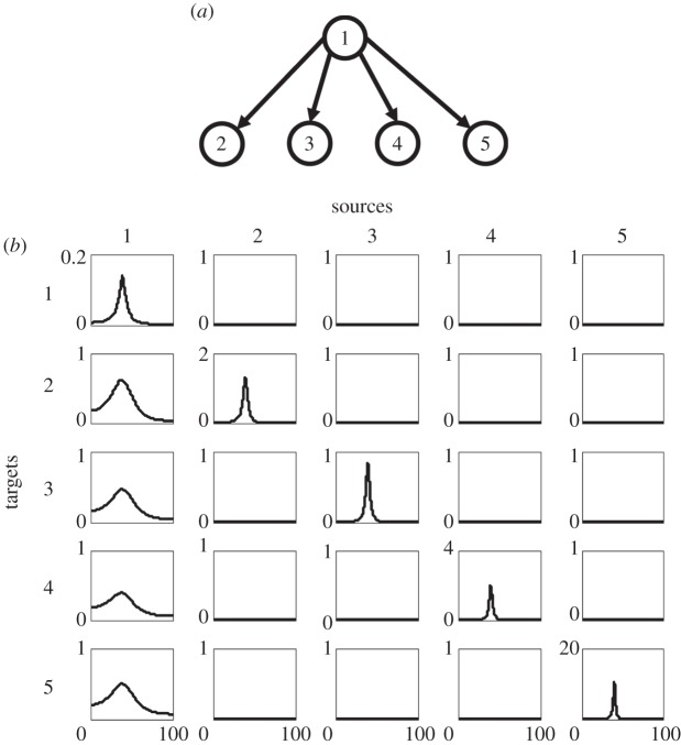
Consider a five-node oscillatory network. The network configuration is shown in figure 1a. The mathematical equations are

3.1

where ε₁(t), ε₂(t), ε₃(t), ε₄(t) and ε₅(t) are independent Gaussian white noise processes with zero means and variances respectively. The intrinsic dynamics of each node is chosen in such a way that they all exhibit a prominent spectral peak at the same frequency. From construction, the signal from the first node (the source) is propagated to the other four nodes (the targets) with differential time delays. A pairwise analysis will reveal non-zero Granger causality from the nodes that receive an early input from the source node to the nodes that receive a late input (e.g. node 3→node 4). Clearly, this does not depict the true connectivity of this dynamical network. Below it will be shown that conditional Granger causality helps to resolve this problem.

Figure 1.

Simulation example 1. (a) Schematic of the network topology and (b) power and conditional Granger causality results from a multivariate parametric analysis.

A dataset of 500 realizations each with 50 time points was generated. The sampling rate is taken to be 200 Hz. Assuming no knowledge of the model equations (3.1), we fitted a fifth-order MVAR model to the simulated dataset and calculated power, coherence and conditional Granger causality spectra from it. In figure 1b, power spectra for all five nodes are shown in panels with the same row and column index, where a spectra peak at around 40 Hz is seen. For the (I,J) panel, where I is the row index that is not equal to the column index J, the conditional Granger causality is from the column index to the row index, namely, J→I. For example, the bottom-left panel is the conditional Granger causality from node 1 to node 5. Only the first column has non-zero conditional Granger causality values, reflecting the driving influence emanating from node 1. The conditional Granger causality among other pairs of nodes is uniformly zero. This corresponds precisely to the structural connectivity pattern in figure 1a. One noteworthy feature about figure 1b is the consistency of spectral features (i.e. peak frequency) across both power and Granger causality spectra. This is important since it allows us to link local dynamics with that of the global network.

(ii). Example 2

A more complex network involving the same five nodes is considered here,

3.2

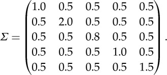
where the noise covariance matrix is

3.3

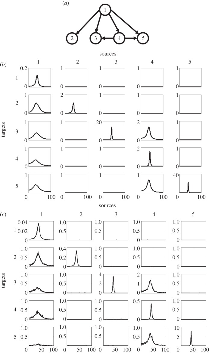
As can be seen, one of the four nodes (node 4) receiving inputs from the source node also transmits information to its nearest neighbours (figure 2a). In addition, the noise terms at different nodes are correlated, giving rise to non-zero instantaneous causality [24].

Figure 2.

Simulation example 2. (a) Schematic of the network topology, (b) power and conditional Granger causality results from a multivariate parametric analysis and (c) results from a non-parametric analysis.

The simulated dataset consists of 200 trials of 500 points each. First, the parametric approach was used. A fifth-order MVAR was fitted to the dataset. The power spectra and conditional Granger causality spectra are shown in figure 2b. Clearly, the structural pattern of this network is correctly recovered by the multivariate Granger causality analysis.

Next, we applied the non-parametric approach described earlier to this example. The power spectra and conditional Granger causality spectra computed with this non-parametric approach are shown in figure 2c. It is seen that this non-parametric approach also correctly recovers the same network connectivity pattern.

(b). Experiment

The 12 attention blocks were rank ordered according to performance accuracy and segmented into 10 groups [10]. Both F_{dACC→rTPJ|dLPFC} and F_{dLPFC→rTPJ|dACC} were calculated for each group, averaged across subjects and plotted as a function of mean group accuracy. The results are shown in figure 3a,b. It can be seen that while F_{dACC→rTPJ|dLPFC} is positively correlated with performance accuracy (Spearman correlation, R=0.82,p<0.01), suggesting that F_{dACC→rTPJ|dLPFC} may represent top-down cognitive control, F_{dLPFC→rIPS|dACC} is not correlated with performance accuracy (R=0.14,p=0.71).

Figure 3.

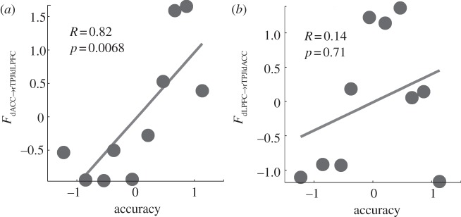
Experimental data: (a,b) conditional Granger causality as a function of performance accuracy.

4. Discussions

Multi-electrode neural recordings and functional imaging are becoming commonplace. Such multivariate data promise unparalleled insights into how different areas of the brain work together to achieve thought and behaviour and how such coordinated brain activity breaks down in disease. While the accumulation of data continues at an astonishing rate, how to effectively analyse these data to extract information about the workings of the brain remains a key challenge. Recent years have witnessed the rapid growth in the applications of various directional measures to multi-channel neural data. The fundamental concept underlying these measures is that of Granger causality. In §2, we presented a brief introduction to this concept with emphasis on Geweke's spectral causality decomposition. For many applications, the spectral representation is necessary as the experimental recordings are replete with oscillatory phenomena. The mathematical development leading to pairwise as well as conditional causality estimations was given in the same section.

Traditionally, Granger causality is estimated via autoregressive models. For multivariate datasets, one has to fit autoregressive models multiple times if one is interested in analysing different combinations of network nodes, increasing the likelihood for estimation errors and model parameter inconsistency. In the proposed formalism, this problem is overcome: a single autoregressive model is fit to all the data and from the overall spectral density matrix, one can select elements corresponding to the subset of channels of interest to form a new spectral density matrix. Since any spectral density matrix can be uniquely factorized into the transfer function and the covariance matrix of the corresponding autoregressive model, Granger causality analysis can be carried out on the subsystem without having to go through a new model fitting process. This spectral density matrix factorization based approach also opens the possibility to extend non-parametric spectral analysis to include Granger causality where the spectral density matrix can be obtained from Fourier or wavelet transforms of data [27,28]. The mathematical expressions for estimating multivariate Granger causality between two channels conditioned on another set of channels were developed in detail.

In practical applications, there is often a need to assess the statistical significance of pairwise and conditional Granger causality values. Past work has employed the random permutation approach for this purpose [2,3,14]. Other methods based on the idea of surrogate data [33,34] or based on the F-test [35] have also been proposed. The functional significance of Granger causality values can be assessed by correlating them with experimental conditions [10].

The effectiveness of Granger causality and the proposed estimation framework was first illustrated on numerical simulations using coupled autoregressive models of varying network complexity. The network configuration identified using our approach is found to agree with the built-in connectivity.

For experimental demonstration, we chose fMRI data recorded from subjects performing a visual spatial attention task [10]. Three ROIs were considered: dACC, right dLPFC and rTPJ. rTPJ is a posterior component of the ventral attention network [31]. Both dACC and dLPFC are thought to be important in maintaining task set and in exerting top-down control over downstream sensorimotor processing [31,32,36]. The exact manner with which the control is achieved is, however, not clear. Our analysis showed that causal influences from dACC to rTPJ conditioned on dLPFC are behaviour enhancing, while causal influences from dLPFC to rTPJ conditioned on dACC have no effects on behaviour. These results appear to suggest that for the current visual spatial attention task, dACC is more important in regulating rTPJ to facilitate task performance.

References

- 1.Valdes-Sosa PA, Sanchez-Bornot JM, Lage-Castellanos A, Vega-Hernandez M, Bosch-Bayard J, Melie-Garcia L, Canales-Rodriguez E. 2005. Estimating brain functional connectivity with sparse multivariate autoregression. Phil. Trans. R. Soc. B 360, 969–981. ( 10.1098/rstb.2005.1654) [DOI] [PMC free article] [PubMed] [Google Scholar]
- 2.Ding M, Chen Y, Bressler SL. 2006. Granger causality: basic theory and applications to neuroscience. Handbook of time series analysis (eds Schelter B, Winterhalder M, Timmer J.), pp. 437–460. Weinheim, Germany: Wiley-VCH Verlag. [Google Scholar]
- 3.Bollimunta A, Chen Y, Schroeder CE, Ding M. 2008. Neuronal mechanisms of cortical alpha oscillations in awake-behaving macaques. J. Neurosci. 28, 9976–9988. ( 10.1523/JNEUROSCI.2699-08.2008) [DOI] [PMC free article] [PubMed] [Google Scholar]
- 4.Goebel R, Roebroeck A, Kim D-S, Formisano E. 2003. Investigating directed cortical interactions in time-resolved fMRI data using vector autoregressive modeling and Granger causality mapping. Magn. Reson. Imaging 21, 1251–1261. ( 10.1016/j.mri.2003.08.026) [DOI] [PubMed] [Google Scholar]
- 5.Hesse W, Möller E, Arnold M, Schack B. 2003. The use of time-variant EEG Granger causality for inspecting directed interdependencies of neural assemblies. J. Neurosci. Methods 124, 27–44. ( 10.1016/S0165-0270(02)00366-7) [DOI] [PubMed] [Google Scholar]
- 6.Kaminski M, Ding M, Truccolo WA, Bressler SL. 2001. Evaluating causal relations in neural systems: Granger causality, directed transfer function and statistical assessment of significance. Biol. Cybern. 85, 145–157. ( 10.1007/s004220000235) [DOI] [PubMed] [Google Scholar]
- 7.Nedungadi A, Rangarajan G, Jain N, Ding M. 2009. Analyzing multiple spike trains with nonparametric Granger causality. J. Comp. Neurosci. 27, 55–64. ( 10.1007/s10827-008-0126-2) [DOI] [PubMed] [Google Scholar]
- 8.Roebroeck A, Formisano E, Goebel R. 2005. Mapping directed influence over the brain using Granger causality and fMRI. Neuroimage 25, 230–242. ( 10.1016/j.neuroimage.2004.11.017) [DOI] [PubMed] [Google Scholar]
- 9.Schelter B, Winterhalder M, Eichler M, Peifer M, Hellwig B, Guschlbauer B, Lücking CH, Dahlhaus R, Timmer J. 2006. Testing for directed influences among neural signals using partial directed coherence. J. Neurosci. Methods 152, 210–219. ( 10.1016/j.jneumeth.2005.09.001) [DOI] [PubMed] [Google Scholar]
- 10.Wen X, Yao L, Liu Y, Ding M. 2012. Causal interactions in attention networks predict behavioral performance. J. Neurosci. 32, 1284–1292. ( 10.1523/JNEUROSCI.2817-11.2012) [DOI] [PMC free article] [PubMed] [Google Scholar]
- 11.Seth AK. 2005. Causal connectivity of evolved neural networks during behavior. Netw. Comp. Neural Syst. 16, 35–54. ( 10.1080/09548980500238756) [DOI] [PubMed] [Google Scholar]
- 12.Baccala LA, Sameshima K. 2001. Partial directed coherence: a new concept in neural structure determination. Biol. Cybern. 84, 463–474. ( 10.1007/PL00007990) [DOI] [PubMed] [Google Scholar]
- 13.Astolfi L, et al. 2005. Assessing cortical functional connectivity by linear inverse estimation and directed transfer function: simulations and application to real data. Clin. Neurophysiol. 116, 920–932. ( 10.1016/j.clinph.2004.10.012) [DOI] [PubMed] [Google Scholar]
- 14.Brovelli A, Ding M, Ledberg A, Chen Y, Nakamura R, Bressler SL. 2004. Beta oscillations in a large-scale sensorimotor cortical network: directional influences revealed by Granger causality. Proc. Natl Acad. Sci. USA 101, 9849–9854. ( 10.1073/pnas.0308538101) [DOI] [PMC free article] [PubMed] [Google Scholar]
- 15.Chen Y, Bressler SL, Ding M. 2006. Stochastic modeling of neurobiological time series: power, coherence, Granger causality, and separation of evoked responses from ongoing activity. Chaos 16, 026113( 10.1063/1.2208455) [DOI] [PubMed] [Google Scholar]
- 16.Chen YH, Bressler SL, Ding MZ. 2006. Frequency decomposition of conditional Granger causality and application to multivariate neural field potential data. J. Neurosci. Methods 150, 228–237. ( 10.1016/j.jneumeth.2005.06.011) [DOI] [PubMed] [Google Scholar]
- 17.Blinowska KJ, Kus R, Kaminski M. 2004. Granger causality and information flow in multivariate processes. Phys. Rev. E 70, 050902( 10.1103/PhysRevE.70.050902) [DOI] [PubMed] [Google Scholar]
- 18.Deshpande G, Laconte S, James GA, Peltier S, Hu X. 2009. Multivariate Granger causality analysis of fMRI data. Hum. Brain Mapp. 30, 1361–1373. ( 10.1002/hbm.20606) [DOI] [PMC free article] [PubMed] [Google Scholar]
- 19.Mader W, Feess D, Lange R, Saur D, Glauche V, Weiller C, Timmer J, Schelter B. 2008. On the detection of direct directed information flow in fMRI. IEEE J. Sel. Top. Signal Process 2, 965–974. ( 10.1109/JSTSP.2008.2008260) [DOI] [Google Scholar]
- 20.Schelter B, Timmer J, Eichlere M. 2009. Assessing the strength of directed influences among neural signals using renormalized partial directed coherence. J. Neurosci. Methods 179, 121–130. ( 10.1016/j.jneumeth.2009.01.006) [DOI] [PubMed] [Google Scholar]
- 21.Wiener N. 1956. The theory of prediction. Modern mathematics for the engineer, (ed. Beckenbach EF.), pp. 165–190. New York, NY: McGraw-Hill. [Google Scholar]
- 22.Granger C. 1969. Investigating causal relations by econometric models and cross-spectral methods. Econometrica 37, 424–438. ( 10.2307/1912791) [DOI] [Google Scholar]
- 23.Geweke J. 1982. Measurement of linear dependence and feedback between multiple time series. J. Am. Stat. Assoc. 77, 304–313. ( 10.1080/01621459.1982.10477803) [DOI] [Google Scholar]
- 24.Geweke J. 1984. Measures of conditional linear dependence and feedback between time series. J. Am. Stat. Assoc. 79, 907–915. ( 10.1080/01621459.1984.10477110) [DOI] [Google Scholar]
- 25.Jenkins GM, Watts DG. 1968. Spectral analysis and its applications. San Francisco, CA: Holden-Day. [Google Scholar]
- 26.Wilson GT. 1972. The factorization of matricial spectral densities. SIAM J. Appl. Math. 23, 420–426. ( 10.1137/0123044) [DOI] [Google Scholar]
- 27.Dhamala M, Rangarajan G, Ding MZ. 2008. Estimating Granger causality from Fourier and wavelet transforms of time series data. Phys. Rev. Lett. 100, 018701 ( 10.1103/PhysRevLett.100.018701) [DOI] [PubMed] [Google Scholar]
- 28.Dhamala M, Rangarajan G, Ding MZ. 2008. Analyzing information flow in brain networks with nonparametric Granger causality. NeuroImage 41, 354–362. ( 10.1016/j.neuroimage.2008.02.020) [DOI] [PMC free article] [PubMed] [Google Scholar]
- 29.Thomson DJ. 1982. Spectrum estimation and harmonic analysis. Proc. IEEE 70, 1055–1096. ( 10.1109/PROC.1982.12433) [DOI] [Google Scholar]
- 30.Walden AT. 2000. A unified view of multitaper spectral estimation. Biometrika 87, 767–788. ( 10.1093/biomet/87.4.767) [DOI] [Google Scholar]
- 31.Corbetta M, Patel G, Shulman GL. 2008. The reorienting system of the human brain: from environment to theory of mind. Neuron 58, 306–324. ( 10.1016/j.neuron.2008.04.017) [DOI] [PMC free article] [PubMed] [Google Scholar]
- 32.Dosenbach NU, et al. 2006. A core system for the implementation of task sets. Neuron 50, 799–812. ( 10.1016/j.neuron.2006.04.031) [DOI] [PMC free article] [PubMed] [Google Scholar]
- 33.Faes L, Pinna GD, Porta A, Maestri R, Nollo G. 2004. Surrogate data analysis for assessing the significance of the coherence function. IEEE Trans. Biomed. Eng. 51, 1156–1166. ( 10.1109/TBME.2004.827271) [DOI] [PubMed] [Google Scholar]
- 34.Faes L, Porta A, Nollo G. 2010. Testing frequency-domain causality in multivariate time series. IEEE Trans. Biomed. Eng. 57, 1897–1906. ( 10.1109/TBME.2010.2042715) [DOI] [PubMed] [Google Scholar]
- 35.Bressler SL, Tang W, Sylvester C, Shulman G, Corbetta M. 2008. Top-down control of human visual cortex by frontal and parietal cortex in anticipatory visual spatial attention. J. Neurosci. 28, 10056–10061. ( 10.1523/JNEUROSCI.1776-08.2008) [DOI] [PMC free article] [PubMed] [Google Scholar]
- 36.Cohen JD, Botvinick M, Carter CS. 2000. Anterior cingulate and prefrontal cortex: who's in control?. Nat. Neurosci. 3, 421–423. ( 10.1038/74783) [DOI] [PubMed] [Google Scholar]