

Abstract
Neurons in cold-blooded animals remarkably maintain their function over a wide range of temperatures, even though the rates of many cellular processes increase twofold, threefold, or many-fold for each 10°C increase in temperature. Moreover, the kinetics of ion channels, maximal conductances, and Ca2+ buffering each have independent temperature sensitivities, suggesting that the balance of biological parameters can be disturbed by even modest temperature changes. In stomatogastric ganglia of the crab Cancer borealis, the duty cycle of the bursting pacemaker kernel is highly robust between 7 and 23°C (Rinberg et al., 2013). We examined how this might be achieved in a detailed conductance-based model in which exponential temperature sensitivities were given by Q10 parameters. We assessed the temperature robustness of this model across 125,000 random sets of Q10 parameters. To examine how robustness might be achieved across a variable population of animals, we repeated this analysis across six sets of maximal conductance parameters that produced similar activity at 11°C. Many permissible combinations of maximal conductance and Q10 parameters were found over broad regions of parameter space and relatively few correlations among Q10s were observed across successful parameter sets. A significant portion of Q10 sets worked for at least 3 of the 6 maximal conductance sets (∼11.1%). Nonetheless, no Q10 set produced robust function across all six maximal conductance sets, suggesting that maximal conductance parameters critically contribute to temperature robustness. Overall, these results provide insight into principles of temperature robustness in neuronal oscillators.
Keywords: conductance-based models, electrical coupling, Q10, stomatogastric ganglion, temperature, voltage-dependent currents
Introduction
Temperature is an influential environmental factor that perturbs the rate of most biochemical processes in a near-exponential fashion. The maximal conductance and activation/inactivation rate of ionic currents increase by a factor (the Q10) of ∼2 or more over a 10°C range (Pena et al., 2006; Peloquin et al., 2008; Tang et al., 2010). These Q10 coefficients can be highly variable. For example, the rate of potassium current activation increases approximately twice as quickly as the rate of sodium activation in Xenopus laevis as temperature increases (Frankenhaeuser and Moore, 1963). Temperature therefore perturbs the magnitude and balance of rate constants in all neurons, which has the potential to drastically alter and potentially disrupt circuit function. Indeed, temperature alters the excitability of cultured neurons and acute brain slices (Watson et al., 1997; Masino and Dunwiddie, 1999) and has been used as a tool to manipulate circuit output and animal behavior in vivo (Long and Fee, 2008; Fee and Long, 2011; Goldin et al., 2013). Although these results establish the physiological importance of temperature, our mechanistic understanding of these effects is very incomplete.
Many biological systems in diverse organisms are surprisingly robust to large temperature perturbations (Ruoff et al., 2007). Cold-blooded animals and warm-blooded animals that hibernate have evolved neural circuits that tolerate these changes remarkably well (Thomas et al., 1986; von der Ohe et al., 2006; Robertson and Money, 2012). We used computational modeling to examine temperature robustness in the pyloric central pattern generator (CPG) in the stomatogastric ganglion (STG) of the crab, Cancer borealis. Both in vitro and in vivo experiments have shown that the pyloric motor pattern increases in frequency in response to raised temperature, but maintains its phasing, or relative timing (Tang et al., 2010; Goeritz et al., 2013). This phenomenon, in which certain features of rhythmic behavior are invariant across temperatures, is referred to as “temperature compensation” (Ruoff et al., 2007; Robertson and Money, 2012). Temperature compensation of phase is important for maintaining appropriate motor output, and has been observed in other invertebrate motor networks (Barclay et al., 2002; Katz et al., 2004; Armstrong et al., 2006).
We examined the effects of temperature on a detailed conductance-based model of the pyloric pacemaker kernel (Soto-Treviño et al., 2005). This component of the pyloric CPG produces a rhythmic, single-phased output that tightly maintains its duty cycle over an ∼20°C temperature range (Rinberg et al., 2013). We investigated how tightly tuned model parameters had to be to satisfy this functional constraint and assessed model output over broad regions of Q10 parameter space to determine whether robust models were confined to specific regions of this space or if these parameters were only loosely constrained. We also investigated whether the maximal conductances of intrinsic ionic currents altered the set of permissive Q10 parameters and the overall temperature robustness of the pacemaker.
Materials and Methods
Experimental model.
The model used here consists of four compartments representing two cells, each with a somatic and axonal compartment. These two model cells are used to represent the three cells of the pyloric pacemaker circuit. The pair of pyloric dilator (PD) cells, which are strongly electrically coupled, are modeled as a single cell. The single anterior burster (AB) cell is modeled as a separate cell. The AB and PD model cells are electrically coupled by a nonrectifying gap junction.
At the reference temperature of 11°C, the model is directly adapted from Soto-Treviño et al. (2005), with two exceptions. First, the value for maximal conductance for IA in the AB cell was 21.6 μS, not 200 μS. Second, the activation exponents of IA in the two cells should be: AB = m4 and PD = m3. These discrepancies were discovered through observation of model behavior and verified by checking the source code used in the original study.
The membrane potential, V, evolves as follows:
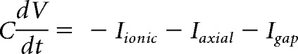 |
where C is the compartment's capacitance, Iionic is the current due to channels in a compartment's membrane, Iaxial is the current flowing between the somatic and axial compartments of a cell, and Igap is current flowing through the gap junction between cells. The voltage-dependent currents included in the model are as follows: sodium (INa), transient calcium (ICaT), slowly inactivating calcium (ICaS), persistant sodium (INaP), hyperpolarization-induced cation current (IH), delayed-rectifier potassium (IKd), calcium-dependent potassium (IKCa), A-type potassium (IA), and the mixed modulatory inward current (IMI).
The current flowing through each conductance is given as follows:
where ḡ is the maximal conductance, mi is the activation variable, hi is the inactivation variable, pi is an integer between 1 and 4, qi is either 0 or 1, and Ei is the reversal potential of the conductance.
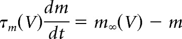
The activation and inactivation variables approach their steady-state values as follows:
 |
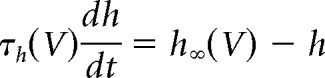 |
where m∞ and h∞ are the steady-state values of the activation and inactivation variables, respectively, and τm and τh are their respective voltage-dependent time constants. These functions are listed in Table 1, along with values for pi and qi.
Table 1.
Voltage and calcium dependence for steady-state (x∞) and time constant (τx) functions for activation (m) and inactivation (h) gating variables
| Cond. | m, h | x∞ | τx (ms) |
|---|---|---|---|
| INa | m3 | ||
| h | |||
| ICaT | m3 | ||
| h | |||
| ICaS | m3 | ||
| INaP | m3 | ||
| h | |||
| Ih | m | ||
| IK | m4 | ||
| IKCa | m4 | ||
| IA | AB: m4 PD: m3 | ||
| h | |||
| IMI | m | 0.5 |
Note that IA activation is m4 in the AB cell and m3 in the PD cell. The variable [Ca] refers to the intracellular calcium concentration (see table 2).
Calcium buffering is implemented as an exponential decay to steady-state as follows:
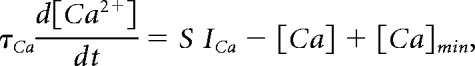 |
where τCa is the time constant for Ca2+ buffering, [Ca] is the internal calcium concentration, and [Ca]min = 0.5 μm is the minimal intracellular Ca2+ concentration. ICa is the total Ca2+ current into the cell through Ca2+ channels in the membrane and S is a constant that converts a current into concentration and is related to the ratio of the surface area of the cell to the volume in which Ca2+ concentration is considered. Table 2 gives the values for necessary parameters involving the calculation of [Ca] and coupling conductances and capacitances for each compartment.
Table 2.
Other parameter values in the model at the reference temperature (11°C)
| AB Cell | PD Cell | |
|---|---|---|
| C | 9.0 nF | 12.0 nF |
| [Ca] | τCa = 303 ms, S = 0.418 μM/nA, Camin = 0.5 μM | τCa = 300 ms, S = 0.515 μM/nA, Camin = 0.5μM |
| Icoup | gaxial = 0.3 μS, ggap = 0.75 μS | gaxial = 1.05 μS, ggap = 0.75 μS |
Icoup refers to the current passing between coupled electrical compartments — gaxial and ggap refer to the soma-axon and soma-soma coupling conductances, respectively (see schematic in Fig. 2). All other symbols are defined in the methods section.
Temperature dependence in the model.
The Q10 temperature coefficient represents the multiplicative change in a parameter over a 10 degree increase in temperature. This can be expressed mathematically as follows:
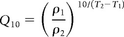 |
where ρ1 denotes the parameter value at temperature T1 and ρ2 denotes the parameter value at temperature T2. We assigned Q10 values for the gating kinetics of ion channels, maximal conductances, compartmental coupling conductances, and the calcium buffering time constant for the pacemaker model described above. The value of a parameter any given temperature T can be calculated given its value at a reference temperature, Tref, by rearranging the equation as follows:
where ρ(T) is the function describing the temperature dependence of a parameter ρ, and ρref is the value of ρ at the reference temperature. For the second equality, we have made the substitution Q(T) = Q10(Tref−T)/10; we refer to Q as the temperature scaling factor. Because the model developed by Soto-Treviño et al. (2005) was fit to experimental data at 11°C, we chose Tref = 11°C.
All conductances (including maximal and compartmental coupling conductances) were directly scaled by the above equation with a Q10 of 1.6, which is representative of published experimental data on the temperature dependence of maximal conductances (Frankenhaeuser and Moore, 1963; Bennetts et al., 2001). The time constants for the activation and inactivation variables (τm and τh) and the time constant of calcium buffering (τCa) were modified by dividing by Q: τ(T) = τref/Q. For the activation and inactivation variables, this is equivalent to scaling the rate constants for the opening and closing of the gate by the same scaling factor Q. The activation and inactivation gating variables follow the standard Hodgkin-Huxley channel model as follows:
 |
 |
where α and β are voltage-dependent functions that represent, respectively, the rates of the forward and backwards chemical reactions. The time constants and steady-state functions for m and h can be shown to equal (Koch, 1999):
 |
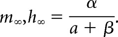 |
We made the simplifying assumption that the Q10 for α and β were always equal because this greatly reduces the number of free parameters in the model and is somewhat supported by experimental data (Frankenhaeuser and Moore, 1963; but see, Voets et al., 2004; Tang et al., 2010). Scaling α and β in the above equations by Q(T) yields the following:
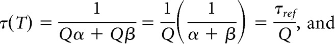 |
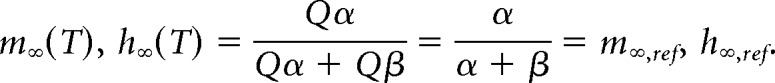 |
Therefore, given our assumptions, the time constant parameters are divided by the temperature scaling factor Q, whereas the steady-state values are insensitive to temperature changes.
Finally, the reversal potentials of all ionic currents were temperature dependent, as specified by the Nernst equation. These changes were relatively small (e.g., ENa increases only 1.76 mV over a 10°C range) and did not appear cause substantial effects on model behavior, but were included for realism. To calculate the reversal potential for the mixed cation channels, IH and IMI, the relative permeabilities of the channel to K+ and Na+ were calculated as follows:
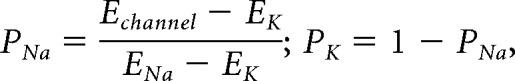 |
where P is the relative permeability of the ion, and E is the reversal potential of the ion or mixed cation channel. These relative permeabilities, along with the reversal potential of Na+ and K+ at the chosen temperature, are used to calculate the reversal potential of these mixed cation channels at that temperature as follows:
Model implementation and data analysis.
The above differential equations were numerically integrated using an exponential Euler method (Dayan and Abbott, 2001). This algorithm was implemented in a custom-written C++ program. Each set of model parameters was simulated for 30 s of model time. We characterized each set of parameters based on the final 15 s of simulation, at which time the models displayed their steady-state behavior.
Duty cycle was calculated by examining the activation of the A current. Burst onset was defined as the point when the activation of the A current passed a set threshold of 0.15 and burst offset was defined as the point then activation of the A current fell below 0.10. This definition was chosen because it closely follows the slow-wave oscillation that drives transmitter release in this system and proved more consistent than definition based on spikes per burst. The duty cycle of tonically firing neurons was set equal to one; the duty cycle of silent neurons was set equal to zero. If the interburst interval was not regular (coefficient of variation <0.05), then the simulation was classified as an irregular burster and was excluded from further analysis. This behavior was quite rare (<0.1% of total).
Data analysis was done in the MATLAB computing environment. The source code for the model has been posted to ModelDB (http://senselab.med.yale.edu/ModelDB/ShowModel.asp?model=152636) and may be used with attribution. MATLAB data analysis scripts are available upon request.
Mathematical analysis of ‘perfect’ temperature scaling.
In the context of the present study, a “perfectly robust” bursting pacemaker is one that precisely maintains its waveform when normalized to cycle period. By definition, such a model would exactly maintain the same duty cycle at any temperature. Mathematically, this means that the limit cycle is invariant to temperature changes, even though the speed of the system along the limit cycle is multiplied by Q. This occurs if the first time derivatives for all state variables (membrane potentials, gating variables, and intracellular calcium), si, are all directly proportional to a common temperature-scaling factor Q as follows:
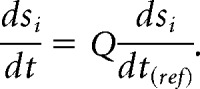 |
Here, is the time derivative of state variable si at the reference temperature (T = 11°C in our study). The above condition implies that the stability and the shape of the limit cycle are invariant to temperature changes; if a vector field is multiplied by a scalar, all trajectories within that field are preserved (though the system moves quicker or slower along them) and the stability of fixed points and limit cycles are unchanged. This condition is not perfectly satisfied in the model, but approximately holds when all Q10 parameters are set equal. We are unaware of any simple mathematical analysis to determine whether a system with unequal Q10 coefficients is temperature compensated. We address this question extensively in the Results section using numerical simulations. If all Q10 parameters are equal, then the above condition holds exactly for all activation gating variables as follows:
 |
An equivalent argument can be trivially made for all inactivation variables, hj, because their dynamics follow the same form as the activation variables.
If we approximate all ionic reversal potentials as being temperature independent, then the membrane potential for each compartment at the reference temperature evolves according to the following:
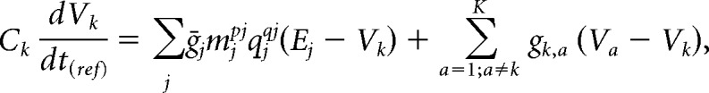 |
where gk,a represents the junctional conductance between the kth and ath electrical compartment and Ck is the capacitance of the compartment. After multiplying all maximal and junctional conductances by Q, we get the following:
 |
The above analysis assumes that all reversal potentials, Ej, do not vary as a function of temperature; however, this is known to be false—the reversal potential of any current is inversely proportional to temperature, as specified by the Nernst equation. Although changes in reversal potentials due to temperature are small (on the order of a few millivolts over a 10°C change), this can potentially have important effects on neuronal activity (Fröhlich et al., 2008). In our model, we did not notice substantial temperature-dependent effects that could be attributed to reversal potential changes (data not shown).
More importantly, the above analysis does not necessarily hold if intracellular calcium or other secondary processes are included in the model. In the pacemaker model analyzed in this paper, the steady-state intracellular calcium, Ca∞, increases in proportion to the total calcium current, ICa, as follows:
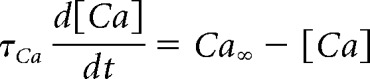 |
 |
Here, Ω represents the set of calcium conductances in an electrical compartment. In our model of temperature, all maximal conductances are multiplied by the temperature coefficient Q and the time constant of Ca2+ buffering is divided by Q. Implementing these changes we get the following:
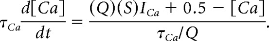 |
Therefore, in our model, the time derivative of [Ca] is not simply changed by a scaling factor, and the model's trajectory is therefore temperature dependent. The effects of intracellular calcium are particularly influential in this model because the calcium-dependent potassium current (IKCa) plays a crucial role in burst termination. Specifically, the temperature-dependent increase in Ca∞ may increase the rate of activation of IKCa and promote early burst termination. If IKCa is activated too quickly, the fast/slow separation of dynamics required for bursting is lost altogether. This analysis is specific to our particular model of intracellular calcium and the details will change depending on the level of biophysical detail that is used (see Discussion).
Results
Temperature robustness across a population of pacemaker models
Figure 1A, left, shows the connectivity of the pyloric CPG circuit. Spontaneous oscillations are dependent on the pacemaker kernel, which consists of two PD neurons and the AB neuron. The lateral pyloric (LP) neuron and pyloric neurons sequentially burst on rebound from the inhibitory synaptic drive delivered by the pacemaker kernel. Therefore, the duty cycle of the pacemaker plays a critical role in determining the phase relationships of the full motor rhythm. The only synaptic feedback onto the pacemaker kernel from the pyloric rhythm is from the LP neuron and it can be blocked pharmacologically by bath application of picrotoxin (Fig. 1A, right; Eisen and Marder, 1982).
Figure 1.

The phasing of the pyloric CPG and the pacemaker kernel are strictly maintained over a range of physiological temperatures. A, Schematic connectivity diagram of the pyloric CPG (left) and isolated pyloric pacemaker kernel (right). The full network contains three motor neuron cell types (PD, LP, and PY) that burst sequentially in a rhythmic pattern to filter food particles in the pylorus. The phasing of this pattern is maintained over a physiological temperature range (Tang et al., 2010). The pacemaker kernel (yellow box) can be pharmacologically isolated by bath application of picrotoxin (PTX), which blocks a subset of inhibitory synapses (in purple). B, Isolated PD neuron bursting increases in frequency but maintains duty cycle in the face of temperature increases (previously published data from Rinberg et al., 2013). Traces in the left column show real-time traces. Traces on the right are normalized to cycle period. Bath temperature is indicated to the left of each trace and increases from cold (blue traces) to hot (red traces). The AB neuron is not shown, but fires in phase with PD. C, Quantification of pacemaker duty cycle as a function of temperature from Rinberg et al. (2013). Error bars represent mean ± SD.
Rinberg et al. (2013) demonstrated that the pharmacologically isolated pacemaker kernel precisely maintained its duty cycle as the bath temperature increased despite increasing in frequency (Fig. 1B,C). We developed a temperature-sensitive model of this system (Fig. 2A) and searched uniformly across Q10 space for models that produced qualitatively similar temperature stability. In addition to varying Q10 parameters, we also varied the maximal conductance densities. It is now well established that models with disparate maximal conductance densities can produce similar behaviors (Goldman et al., 2001; Prinz et al., 2003, 2004; Achard and De Schutter, 2006; Sobie, 2009; Marder and Taylor, 2011; Rathour and Narayanan, 2012; Lamb and Calabrese, 2013). Similar parameter variability is observed in experimental measurements of conductance density (Golowasch et al., 1999; Swensen and Bean, 2005; Schulz et al., 2006, 2007; Goaillard et al., 2009; Tobin et al., 2009; Amendola et al., 2012).
Figure 2.

A temperature-sensitive model of the pyloric pacemaker kernel. A, Schematic diagram of the four-compartment conductance-based model, with voltage-dependent currents listed. B, Six maximal conductance sets that produce biologically realistic and nearly identical bursting patterns at 11°C. Left, Voltage traces for each maximal conductance set (red traces = AB soma; blue traces = PD soma). Right, Corresponding parameters for each maximal conductance set (normalized to parameters for set #0). Kd(a) and Kd(s), respectively, indicate the maximal conductances of delayed rectifier current in the axonal and somatic compartments.
We assessed the temperature robustness of the model for six different maximal conductance sets, all of which produced similar activity at the reference temperature of 11°C (Fig. 2B, Tables 3, 4). The first maximal conductance set (set #0) was identical to the one developed by Soto-Treviño et al. (2005), which was hand tuned to replicate biological behavior both under standard conditions and in response to current injections. We found the other five maximal conductance sets by uniformly searching over maximal conductance space; we selected five maximal conductance sets with simulated activity that was visually similar to that of set #0. Despite producing nearly identical behaviors (Fig. 2B, left, traces), the maximal conductance values were substantially different from each other (Fig. 2B, right, bar plots).
Table 3.
Maximal conductance (μS) and reversal potential (mV) parameters for the AB model neurons at 11 °C
| ḡset0 | ḡset1 | ḡset2 | ḡset3 | ḡset4 | ḡset5 | Ei | |
|---|---|---|---|---|---|---|---|
| Axon | |||||||
| INa | 300 | 412.72 | 355.49 | 508.2 | 446.89 | 426.94 | 50 |
| IK | 52.5 | 23.609 | 71.253 | 5.7604 | 19.444 | 39.732 | −80 |
| IL | 0.0018 | 0.0018 | 0.0018 | 0.0018 | 0.0018 | 0.0018 | −60 |
| Soma | |||||||
| ICaT | 55.2 | 92.765 | 86.892 | 77.159 | 84.658 | 44.078 | |
| ICaS | 9 | 14.07 | 10.904 | 16.814 | 0.87369 | 14.854 | |
| INaP | 2.7 | 2.6022 | 1.4156 | 4.7129 | 0.023004 | 2.9285 | 50 |
| ḡset0 | 0.054 | 0.1061 | 0.036018 | 0.024495 | 0.10645 | 0.040302 | −20 |
| IK | 1890 | 3140.6 | 1903.5 | 3005.1 | 2644 | 2102.3 | −80 |
| IKCa | 6000 | 3686.3 | 9527.5 | 3090.9 | 10913 | 5472.9 | −80 |
| IA | 21.6 | 180.73 | 310.62 | 50.497 | 337.17 | 114.75 | −80 |
| IMI | 570 | 667.35 | 171.99 | 551.69 | 859.7 | 17.69 | 0 |
| IL | 0.045 | 0.045 | 0.045 | 0.045 | 0.045 | 0.045 | −50 |
Six maximal conductance parameter sets were examined (#0–5). Ei is the reversal potential for each ionic current.
Table 4.
Maximal conductance (μS) and reversal potential (mV) parameters for the PD model neurons at 11 °C
| ḡset0 | ḡset1 | ḡset2 | ḡset3 | ḡset4 | ḡset5 | Ei | |
|---|---|---|---|---|---|---|---|
| Axon | |||||||
| INa | 1110 | 1099 | 1582.8 | 1461.3 | 1839.5 | 1327.4 | 50 |
| IK | 150 | 82.305 | 260.74 | 207.05 | 77.218 | 42.142 | −80 |
| IL | 0.00081 | 0.00081 | 0.00081 | 0.00081 | 0.00081 | 0.00081 | −55 |
| Soma | |||||||
| ICaT | 22.5 | 29.923 | 14.933 | 38.2 | 1.1742 | 16.428 | |
| ICaS | 60 | 77.029 | 62.991 | 43.167 | 113.14 | 100.18 | |
| INaP | 4.38 | 5.6932 | 7.2169 | 0.37758 | 7.2664 | 6.5393 | 50 |
| Ih | 0.219 | 0.12909 | 0.13924 | 0.31325 | 0.035045 | 0.19716 | −20 |
| IK | 1576.8 | 2660 | 1081.1 | 1023.9 | 2669.1 | 2946.3 | −80 |
| IKCa | 251.85 | 248.91 | 171 | 405.53 | 378.99 | 489.41 | −80 |
| IA | 39.42 | 41.84 | 38.112 | 78.717 | 26.893 | 55.417 | −80 |
| IL | 0.105 | 0.105 | 0.105 | 0.105 | 0.105 | 0.105 | −55 |
Six maximal conductance parameter sets were examined (#0–5). Ei is the reversal potential for each ionic current.
We then randomly generated 125,000 distinct Q10 sets for the time constants of channel gating and calcium buffering; each Q10 was randomly drawn from a uniform distribution from 1 to 4. A Q10 coefficent of 1.6 was assigned to all maximal conductances, gap junction conductances, and axial conductances (see Materials and Methods). We simulated each of the six maximal conductance sets with all 125,000 Q10 sets. The same Q10 sets were applied to each maximal conductance set to make individual cases directly comparable. This also removed any possible inconsistencies that using different Q10s for different maximal conductance sets might introduce. We also simulated maximal conductance set #0 (same as Soto-Treviño et al., 2005) with an additional 125,000 randomly selected Q10 sets, bringing the total to 825,000 parameter sets (all combinations of Q10 sets and maximal conductance sets). We simulated the additional 125,000 Q10 sets for maximal conductance set #0 to ensure that we had sampled Q10 space densely enough for the remaining maximal conductance sets.
For each combination of Q10 and maximal conductance parameters, we simulated model output at five different physiological temperatures (7°C, 11°C, 15°C, 19°C, and 23°C). Models with irregular bursting were quite rare (<0.1% of total) and were excluded from further analysis. We observed a range of model behaviors (Fig. 3A) that were consistent with preliminary modeling work from a previous study (Tang et al., 2010). Although some individual models maintained their duty cycle robustly over this temperature range (Fig. 3A, “pass”), other individual models were fragile to temperature perturbations (Fig. 3A, “fail”).
Figure 3.

Quantification of duty cycle maintenance over a physiological temperature range across all maximal conductance sets and Q10 parameter sets. A, Example voltage traces for models that “passed” and “failed” our criterion for maintaining a stable duty cycle (red traces = AB soma; blue traces = PD soma). B, Distribution of total sum of squares variability for burst duty cycle (see text) for each maximal conductance set. Black bars represent models that burst at all temperatures. Blue bars represent models that failed to burst at one temperature. Green bars represent models that failed to burst at two temperatures. Red bars represent models that failed to burst at three or four temperatures.
We quantified the variability of pacemaker duty cycle as the total sum of squares difference (SST) from the duty cycle at the reference temperature of 11°C as follows:
 |
Lower SSTDC values correspond to greater robustness (less variability in duty cycle). Figure 3B displays the distribution of this metric over all Q10 sets for each maximal conductance set. Importantly, the chances of finding a Q10 set that produced a robust oscillator varied across maximal conductance sets. The distributions for maximal conductance sets #1 and #3 tended toward lower (more robust) SSTDC values than the distributions of sets #4 and #5.
The black histograms in Figure 3B are those individual models that burst over the entire temperature range. Those to the left of the dashed red line maintained approximately constant duty cycle, whereas those to the right of the red line failed to do so. The blue histograms include those models that failed to burst at one temperature, the green models failed to burst at two temperatures, and the red models failed at three temperatures. In this figure, all simulated Q10 sets are shown for maximal conductance set #0, which is twice as many compared with the other maximal conductance sets.
Analysis of robust parameter sets
We performed further analysis on all individual models that produced an SSTDC <0.01 (Fig. 3B, models to the left of the dashed red lines in each maximal conductance set). Simulations within this subpopulation were fairly robust to temperature changes and were considered to be “successful” models. Although this threshold was somewhat arbitrarily chosen, changing it to be more or less restrictive did not qualitatively change the results. Likewise, using an alternative measure of oscillator robustness that was based on the number of spikes per burst rather than duty cycle did not substantially alter our results (Caplan, 2013).
To understand which Q10s were most influential in conferring temperature robustness to the models, we plotted histograms of each Q10 parameter value within the subset of successful models (Fig. 4). All Q10 sets were originally drawn from a uniform distribution; therefore, flat histograms in Figure 4 correspond to Q10 parameters that were equally likely to produce robust oscillators across the entire sampled interval, whereas peaks (or troughs) of nonflat distributions show the values of Q10s that were likely (or, respectively, unlikely) to be found in the successful models. For example, robust oscillations were more likely to be seen if the Q10 for mKCa was small, because the distribution for this parameter is shifted to the left across all six maximal conductance sets.
Figure 4.

Distributions of Q10 parameters in models displaying temperature compensation of duty cycle (SSTDC < 0.01). Each row corresponds to one of the six maximal conductance parameter sets. Each column corresponds to a different Q10 parameter in the model. Yellow boxes highlight six Q10parameters that had noticeably nonuniform distributions. Histogram peaks correspond to parameter values that typically supported compensation. Troughs correspond to parameter values that typically disrupted compensation. The vertical scales on the histograms are consistent across each row (same maximal conductance set), but differ between rows. The purpose of these plots is to illustrate the shape of the distributions rather than their amplitudes, so the vertical axis has been omitted for clarity.
Interestingly, when viewed on an individual basis, most Q10 parameters had qualitatively similar effects across many or all maximal conductance sets. The Q10s for mNa, hCaT, mNaP, hNaP, mH, mA, hA, and mMI displayed flat distributions across all maximal conductance sets (shown in white)—that is, they did not noticeably influence the model's ability to maintain a constant duty cycle (looking down the six rows, the results are similar). In yellow are the Q10s that were influential in at least one maximal conductance set. The Q10s for mKCa and the time constant for calcium buffering had typically lower values in robust oscillators for all conductance sets, whereas the Q10 for mCaT was typically lower for conductance sets #1–4, but noninfluential (flat) in set #5. The Q10s for hNa, mKd, and mCaS showed qualitatively opposite effects across some of the maximal conductance sets. For example, the Q10 distribution for mKd in Figure 4 is shifted toward higher values in all maximal conductance sets but #4, in which it is shifted toward lower values.
We next examined the pairwise interactions between the six particularly influential Q10 parameters (highlighted in Fig. 4) in the subpopulation of successful models. In Figure 5, the histograms along the diagonal of each panel show the individual distributions for these Q10s (same as the histograms in Fig. 4). The blue-to-red heat maps above the diagonal of each panel show the joint distribution of successful models for each pair of Q10 parameters; these are 2D histograms for each pair of Q10s, with red representing areas of relatively high density of robust models and blue representing areas with relatively few successful models. It is important to note that viable Q10 sets are spread over large regions of parameter space; they are not tightly confined to specific regions and few strong correlations are observed.
Figure 5.

Pairwise distributions for six influential Q10 parameters in robust models (SSTDC < 0.01) shown for all six maximal conductance parameter sets (#0–5). Histograms along the diagonal show the individual Q10 distributions (as in Fig. 5). These are estimates of marginal probability distributions, p(x) for each Q10 parameter. Blue-to-red plots above the histograms are 2D histograms showing all pairwise distributions (red areas = high density, blue areas = low density). These are estimates of joint probability distributions, p(x,y), for each pair of Q10 parameters. Blue-to-gray-to-pink plots below the histograms show the difference between the observed joint distribution and the expected joint distribution under the assumption of that the two marginal distributions are independent events; that is, these show the quantity p(x,y) − p(x)p(y). Pink and blue areas represent regions where there were more or fewer solutions than expected, respectively. All color scales are consistent within panels, but are scaled between panels to illustrate the trends independent of the total number of successful models in each maximal conductance set.
The blue-to-gray-to-pink heat maps below the diagonal on each were calculated by subtracting the product of the two individual distributions (histograms on diagonal) from the joint distribution (plots above diagonal). If the two Q10s were completely independently distributed, this would produce a value of zero (gray) in each bin. Magenta areas denote positive values, bins that hold more successful models than is predicted by assuming the two individual distributions are independent. Blue areas denote negative values, bins that hold fewer successful models than expected. One can also interpret these plots as a representation of the information gained from considering the joint distribution of two Q10s rather than their separate individual distributions; little additional information is gained in uniformly gray plots, whereas more is gained in plots that have substantial pink and blue patches. These plots are useful to visualize correlations that are not easily perceptible in the joint distribution plots.
As in Figure 4, many similar features can be seen in Figure 5 across the six maximal conductance sets. Most differences arise from the fact that maximal conductance set #4 and #5 have fewer successful models than sets #0–3 and therefore have sparser distributions. A particularly striking relationship is present between the Q10s for mKCa and calcium buffering; a downward sloping pink curve in the plots below the diagonal for all conductance sets. Other patterns are similarly visible across the maximal conductance sets (e.g., the positive correlation between the Q10s for mCaS and calcium buffering). An exception is the positive correlation between mCaS and mKd in set #4, which is not easily seen in any of the other maximal conductance sets.
No Q10 sets produced robust oscillators across all maximal conductance sets
To understand whether the Q10 combinations that work for individual maximal conductance sets are unique to that maximal conductance set or if they provide more general solutions that can work for many maximal conductance sets, we investigated whether there are Q10 sets that satisfied SSTDC < 0.01 for multiple maximal conductance sets.
No Q10 set satisfied this criterion for all maximal conductance sets. When we required that a model work for 5 of the 6 conductance sets, only ∼1.2% of Q10s passed this criterion (Fig. 6A). Given the dense sampling of Q10 parameter space, this result suggests that it is difficult (and perhaps biologically implausible) to find a set of Q10 values that supports temperature compensation for all viable maximal conductance sets. Therefore, tuning maximal conductances appears to be important for designing neuronal systems that are robust to temperature perturbations.
Figure 6.

Distributions of Q10 parameter sets that produced robust models for at least five (A), three (B), or one (C), maximal conductance sets. Plots are constructed in the same manner as in Figure 5.
Next, we relaxed the test by requiring that each Q10 set only pass in 3 of 6 conductance sets (Fig. 6B). Approximately 11.1% of the Q10 sets passed this criterion. These Q10 sets were distributed similarly to the Q10 sets that produced temperature compensation for each maximal conductance set (cf. Fig. 5). We then examined Q10 sets that worked for any one of the six maximal conductance sets (Fig. 6C). Only ∼36.2% of Q10 sets satisfied this relaxed criterion. Overall, these results suggest that many Q10sets are incompatible with temperature compensation of duty cycle regardless of underlying maximal conductance profile of the neuron. This suggests that there exists a subset of nonpermissible Q10 parameters that cannot be compensated for by tuning maximal conductances. Overall, Figure 6 suggests that both maximal conductances and Q10 parameters must fall within certain ranges to produce temperature robustness across a variable population of models. This suggests that both of these parameters types may be tuned by evolutionary or other processes (see Discussion).
Do Q10s have to be similar to produce robust temperature scaling?
In principle, if all of the Q10s in a complex model were identical, one would get close to perfect temperature scaling (see Materials and Methods; Robertson and Money, 2012). This raises the question of whether models with Q10s more similar to each other are, on average, more robust than models with dissimilar Q10s.
We calculated the coefficient of variation (CV) for the Q10 parameters to quantify the level of similarity within each Q10 set. The CV is the corrected sample SD normalized to the sample mean; large values correspond to dissimilar Q10 sets and small values correspond to sets in which Q10 coefficients are all similar. Surprisingly, this variable held extremely little predictive power for the robustness of the oscillator as measured by SSTDC; the coefficient of determination (R2) between these two variables was <0.01 for all maximal conductance sets. This was true even if we calculated the CV only across the six “influential” Q10s highlighted in Figure 5 and further analyzed in Figure 6 (data not shown), suggesting that this result does not simply arise from variability in the deconstrained Q10 parameters (i.e., the ones not highlighted in Fig. 5). We also did not find notable relationships between oscillator robustness and alternative measures of Q10 variability such as the interquartile range, which is a robust measure of variability in the presence of outliers (data not shown).
Therefore, we conclude that one cannot determine the robustness of a Q10 set simply by inspecting the similarity of the Q10 coefficients. This result is illustrated in Figure 7, which shows the distribution of the CV for all Q10 sets in each maximal conductance set. Note that the CV for the robust Q10 sets (blue histograms; SSTDC < 0.01) were similarly distributed to the CV of all simulated Q10 sets (red histograms). If robust models were more likely to have similar Q10 values, the blue histograms would have been shifted to the left with respect to the red histograms.
Figure 7.

Distributions of Q10 set similarity (coefficient of variation, CV) for all sampled Q10 sets (red histograms) and all robust Q10 sets (SSTDC < 0.01; blue histograms) for each maximal conductance set. Colored arrows indicate the mean of each distribution. The similarity of each set of Q10 values was quantified by the CV. If having similar Q10s (low CV) was associated with more reliable temperature compensation, the blue histograms (robust Q10 sets) would be shifted to the left of the red histograms (all sampled Q10 sets).
Discussion
Acute temperature changes are global perturbations that simultaneously alter many cellular processes and can therefore disrupt neuronal function (Robertson and Money, 2012; Tang et al., 2012). Animals have evolved to flourish despite significant daily and seasonal changes in temperature using compensatory mechanisms that work well, even if they remain mysterious to us. Cold-blooded animals also regulate their body temperature through behavioral preferences (Lagerspetz and Vainio, 2006; Garrity et al., 2010; Sengupta and Garrity, 2013) and acclimate physiologically to long-term temperature changes over days, weeks, or months (Camacho et al., 2006; Garrett and Rosenthal, 2012b; Tang et al., 2012).
In contrast to long-term adaptation or active tuning, this study examines the intrinsic robustness of neural systems to acute temperature perturbations. We specifically focused on temperature compensation of duty cycle in the pyloric pacemaker kernel of the crustacean STG (Rinberg et al., 2013). A number of other invertebrate circuits also show temperature compensation of phase, including the circuits controlling Tritonia swimming (Katz et al., 2004), Drosophila larval crawling (Barclay et al., 2002), and locust ventilation (Armstrong et al., 2006).
We examined a population of temperature-sensitive computational models by varying Q10 and maximal conductance parameters. Our results address two major issues: (1) how a rhythmic dynamical system can maintain its phasing (or duty cycle if single-phase) despite having many components with highly variable temperature sensitivities, and (2) how temperature robustness can be achieved reliably across an intrinsically variable population of neurons (Swensen and Bean, 2005; Schulz et al., 2006, 2007; Goaillard et al., 2009; Tobin et al., 2009; Amendola et al., 2012; Roffman et al., 2012).
An important result is that the same sets of Q10s do not uniformly produce temperature compensation across the six maximal conductance sets we examined. No Q10 set worked for all maximal conductance sets; however, a reasonable fraction of Q10 sets (∼11%) worked for at least three maximal conductance sets. This strongly suggests that both maximal conductances and Q10 parameters must be tuned in biological systems that display robust temperature compensation. One possibility is that Q10s and conductance densities are coregulated during development and the lifetime of the animal to ensure that they are appropriately matched. Alternatively, Q10 coefficients may be genetically determined and fixed over an animal's lifetime. In this case, developmental mechanisms must establish a maximal conductance profile that both produces appropriate activity and is well matched to the Q10 parameters. In turn, the Q10s may have been tuned over evolutionary timescales to accommodate variable conductance expression.
Ion channel protein structure determines the Q10 of channel activation and inactivation (Zheng, 2013). Mutagenic analyses of the canonical heat-sensing channel TRPV1 have demonstrated that temperature sensitivity varies dramatically as protein structure and composition are manipulated (Vlachová et al., 2003; Brauchi et al., 2006; Yao et al., 2011). Therefore, one might imagine that minor allelic fluctuations in ion channel proteins found in the wild-type population produce animal-to-animal variations in the Q10s for some channel proteins. This would allow these parameters to be tuned over many generations by natural selection. To our knowledge, the extent of animal-to-animal variability in Q10 parameters has not been characterized experimentally in detail.
Neurons may also have the ability to actively regulate Q10 parameters to foster temperature stability. Indeed, crabs acclimated at 19°C are less susceptible to circuit “crashes” at high temperatures than crabs acclimated at 7 or 11°C (Tang et al., 2012). Our results suggest this could be achieved by tuning maximal conductance parameters, perhaps through homeostatic regulatory pathways (Liu et al., 1998; Turrigiano, 2011; Davis, 2013; Williams et al., 2013). It is also plausible that these neurons tune their channel Q10s to achieve greater robustness; this could potentially be achieved by altering ion channel composition through posttranslational modifications, RNA editing, or altering the relative expression of ion channel subtypes. If this were the case, then it is also possible that maximal conductances are coregulated with channel Q10 parameters.
Other possible mechanisms for biological temperature robustness
The robustness of a neuron to temperature perturbations is partially dependent on its Q10 parameters. We also show that maximal conductance parameters strongly influence temperature robustness. In addition to tuning maximal conductances, neurons might also manipulate the voltage and time dependence of ionic currents to support robust function. Indeed, this strategy appears to be used by polar octopus species that use RNA editing to express K+ channel isoforms with accelerated gating kinetics relative to tropical octopus species (Garrett and Rosenthal, 2012a). Intriguingly, RNA-editing mechanisms have been proposed to promote long-term temperature robustness within individual animals (temperature acclimation) in addition to explaining these cross-species differences (Garrett and Rosenthal, 2012b).
Tuning intracellular Ca2+ regulation is another potential mechanism to improve neural robustness. Intracellular Ca2+ is controlled by a rich set of temperature-dependent processes, such as sequestration into internal compartments or by chemical chelators (Berridge et al., 2000). We did not attempt to model these details because they are still poorly characterized within crustacean stomatogastric neurons. Nevertheless, given the influential nature of intracellular Ca2+ in our results, tuning these regulatory pathways is another potential mechanism for achieving temperature robustness.
Importance of intracellular calcium dynamics to temperature robustness
The Q10 coefficients for mKCa and the time constant for calcium buffering were particularly important for establishing temperature stability in these models. This result likely stems from the fact that both of these parameters strongly influence IKCa, which plays a critical role in terminating each burst (Soto-Treviño et al., 2005). Because the steady-state intracellular calcium level (Ca∞) increases with temperature (see Materials and Methods), IKCa is likely to activate earlier in the burst phase at higher temperatures and disrupt the burst duty cycle. Models with low Q10 coefficients for mKCa and τCa were overrepresented in the successful subset of simulated models, suggesting at least two possible compensations for this disruption. These results are consistent with a simple conceptual model, in which several degenerate model parameters contribute to the temperature dependence of IKCa and, by extension, duty cycle constancy.
A previous study (Rinberg et al., 2013) examined temperature stability in a Morris-Lecar oscillator as a reduced model of the pyloric pacemaker kernel. This simple model also predicted that disparate maximal conductance sets would produce variable responses to temperature perturbations, even when consistent Q10 sets are used. Rinberg et al.'s (2013) results suggested that the Q10 coefficients for the time constants of outward currents should be generally larger than the Q10s for inward current gates in robust models; however, we did not observe this. This discrepancy may result from the intracellular Ca2+ dynamics that are absent in the Morris-Lecar model, but were present in the detailed model analyzed herein.
General lessons for parameter fitting
Finding appropriate parameter values for neuron and network models is a longstanding problem in computational neuroscience. A successful approach for moderately sized models has been to randomly search parameter space for models that match biological data by some set of physiological measures (Goldman et al., 2001; Prinz et al., 2003, 2004; Achard and De Schutter, 2006; Taylor et al., 2009; Ball et al., 2010; Rathour and Narayanan, 2012; Lamb and Calabrese, 2013). Models that satisfy these constraints are considered “successful.” This population-based approach prevents investigators from studying the idiosyncrasies of individual parameter sets (Marder and Taylor, 2011).
One concern with this approach has been that biological neurons are subject to more constraints than are typically considered by investigators; therefore, these modeling studies may be too lenient and overestimate the number of feasible parameter sets (Nowotny et al., 2007). In this study, we considered effective temperature compensation as an additional biological constraint. This additional constraint suggests that certain maximal conductance sets may not be feasible solutions, even if they appear “successful” at 11°C. However, we still uncovered a large and widely spread population of successful parameter sets (∼12.5% of all simulated sets) by searching over both maximal conductance and Q10 parameter space.
Incorporating further constraints into a model (e.g., temperature) can introduce more free parameters. Here, we added many Q10 parameters to make the model temperature dependent and found many feasible models within this expanded parameter space. Although biological systems probably do not explore this entire space of possible solutions (O'Leary et al., 2013), computational modeling can provide insight by exploring this larger space. Biological systems ultimately find solutions in high-dimensional parameter spaces because they must simultaneously satisfy many complex functional constraints (Brezina and Weiss, 1997). In addition to temperature compensation, other constraints could include reliable neuromodulation (Grashow et al., 2009, 2010), energy efficiency (Laughlin and Sejnowski, 2003), and gain control (Abbott et al., 1997). Our results emphasize that there are multiple mechanisms for neurons to achieve temperature compensation (and presumably other constraints). This contrasts with the intuition one might gain from studying reduced models, which typically identify a handful of “critical” variables. This illustrates the utility of comparing results from models with varying degrees of complexity and detail.
Footnotes
This work was supported by the NIH (Grant NS 081013). We thank Tilman Kispersky and Timothy O'Leary for providing helpful feedback on an early draft of this manuscript.
The authors declare no competing financial interests.
References
- Abbott LF, Varela JA, Sen K, Nelson SB. Synaptic depression and cortical gain control. Science. 1997;275:220–224. doi: 10.1126/science.275.5297.221. [DOI] [PubMed] [Google Scholar]
- Achard P, De Schutter E. Complex parameter landscape for a complex neuron model. PLoS Comput Biol. 2006;2:e94. doi: 10.1371/journal.pcbi.0020094. [DOI] [PMC free article] [PubMed] [Google Scholar]
- Amendola J, Woodhouse A, Martin-Eauclaire MF, Goaillard JM. Ca2+/cAMP-sensitive covariation of IA and IH voltage dependences tunes rebound firing in dopaminergic neurons. J Neurosci. 2012;32:2166–2181. doi: 10.1523/JNEUROSCI.5297-11.2012. [DOI] [PMC free article] [PubMed] [Google Scholar]
- Armstrong GA, Shoemaker KL, Money TG, Robertson RM. Octopamine mediates thermal preconditioning of the locust ventilatory central pattern generator via a cAMP/protein kinase A signaling pathway. J Neurosci. 2006;26:12118–12126. doi: 10.1523/JNEUROSCI.3347-06.2006. [DOI] [PMC free article] [PubMed] [Google Scholar]
- Ball JM, Franklin CC, Tobin AE, Schulz DJ, Nair SS. Coregulation of ion channel conductances preserves output in a computational model of a crustacean cardiac motor neuron. J Neurosci. 2010;30:8637–8649. doi: 10.1523/JNEUROSCI.6435-09.2010. [DOI] [PMC free article] [PubMed] [Google Scholar]
- Barclay JW, Atwood HL, Robertson RM. Impairment of central pattern generation in Drosophila cysteine string protein mutants. J Comp Physiol A Neuroethol Sens Neural Behav Physiol. 2002;188:71–78. doi: 10.1007/s00359-002-0279-9. [DOI] [PubMed] [Google Scholar]
- Bennetts B, Roberts ML, Bretag AH, Rychkov GY. Temperature dependence of human muscle ClC-1 chloride channel. J Physiol. 2001;535:83–93. doi: 10.1111/j.1469-7793.2001.t01-1-00083.x. [DOI] [PMC free article] [PubMed] [Google Scholar]
- Berridge MJ, Lipp P, Bootman MD. The versatility and universality of calcium signalling. Nat Rev Mol Cell Biol. 2000;1:11–21. doi: 10.1038/35036035. [DOI] [PubMed] [Google Scholar]
- Brauchi S, Orta G, Salazar M, Rosenmann E, Latorre R. A hot-sensing cold receptor: C-terminal domain determines thermosensation in transient receptor potential channels. J Neurosci. 2006;26:4835–4840. doi: 10.1523/JNEUROSCI.5080-05.2006. [DOI] [PMC free article] [PubMed] [Google Scholar]
- Brezina V, Weiss KR. Analyzing the functional consequences of transmitter complexity. Trends Neurosci. 1997;20:538–543. doi: 10.1016/S0166-2236(97)01120-X. [DOI] [PubMed] [Google Scholar]
- Camacho J, Qadri SA, Wang H, Worden MK. Temperature acclimation alters cardiac performance in the lobster Homarus americanus. J Comp Physiol A Neuroethol Sens Neural Behav Physiol. 2006;192:1327–1334. doi: 10.1007/s00359-006-0162-1. [DOI] [PubMed] [Google Scholar]
- Caplan JS. Neuroscience Department, Brandeis University; 2013. Temperature scaling in pyloric networks: A computational study of a small neural network oscillator and the effects of ion channel temperature dependencies on network performance. PhD Thesis. [Google Scholar]
- Davis GW. Homeostatic signaling and the stabilization of neural function. Neuron. 2013;80:718–728. doi: 10.1016/j.neuron.2013.09.044. [DOI] [PMC free article] [PubMed] [Google Scholar]
- Dayan P, Abbott LF. Theoretical neuroscience. Cambridge: MIT; 2001. [Google Scholar]
- Eisen JS, Marder E. Mechanisms underlying pattern generation in lobster stomatogastric ganglion as determined by selective inactivation of identified neurons. III. Synaptic connections of. J Neurophysiol. 1982;48:1392–1415. doi: 10.1152/jn.1982.48.6.1392. [DOI] [PubMed] [Google Scholar]
- Fee MS, Long MA. New methods for localizing and manipulating neuronal dynamics in behaving animals. Curr Opin Neurobiol. 2011;21:693–700. doi: 10.1016/j.conb.2011.06.010. [DOI] [PMC free article] [PubMed] [Google Scholar]
- Frankenhaeuser B, Moore LE. The effect of temperature on the sodium and potassium permeability changes in myelinated nerve fibres of Xenopus laevis. J Physiol. 1963;169:431–437. doi: 10.1113/jphysiol.1963.sp007269. [DOI] [PMC free article] [PubMed] [Google Scholar]
- Fröhlich F, Bazhenov M, Iragui-Madoz V, Sejnowski TJ. Potassium dynamics in the epileptic cortex: new insights on an old topic. Neuroscientist. 2008;14:422–433. doi: 10.1177/1073858408317955. [DOI] [PMC free article] [PubMed] [Google Scholar]
- Garrett S, Rosenthal JJ. RNA editing underlies temperature adaptation in K+ channels from polar octopuses. Science. 2012a;335:848–851. doi: 10.1126/science.1212795. [DOI] [PMC free article] [PubMed] [Google Scholar]
- Garrett SC, Rosenthal JJC. A role for A-to-I RNA editing in temperature adaptation. Physiol. 2012b;27:362–369. doi: 10.1152/physiol.00029.2012. [DOI] [PMC free article] [PubMed] [Google Scholar]
- Garrity PA, Goodman MB, Samuel AD, Sengupta P. Running hot and cold: behavioral strategies, neural circuits, and the molecular machinery for thermotaxis in C. elegans and Drosophila. Genes Dev. 2010;24:2365–2382. doi: 10.1101/gad.1953710. [DOI] [PMC free article] [PubMed] [Google Scholar]
- Goaillard JM, Taylor AL, Schulz DJ, Marder E. Functional consequences of animal-to-animal variation in circuit parameters. Nat Neurosci. 2009;12:1424–1430. doi: 10.1038/nn.2404. [DOI] [PMC free article] [PubMed] [Google Scholar]
- Goldin MA, Alonso LM, Alliende JA, Goller F, Mindlin GB. Temperature induced syllable breaking unveils nonlinearly interacting timescales in birdsong motor pathway. PLoS One. 2013;8:e67814. doi: 10.1371/journal.pone.0067814. [DOI] [PMC free article] [PubMed] [Google Scholar]
- Goldman MS, Golowasch J, Marder E, Abbott LF. Global structure, robustness, and modulation of neuronal models. J Neurosci. 2001;21:5229–5238. doi: 10.1523/JNEUROSCI.21-14-05229.2001. [DOI] [PMC free article] [PubMed] [Google Scholar]
- Golowasch J, Abbott LF, Marder E. Activity-dependent regulation of potassium currents in an identified neuron of the stomatogastric ganglion of the crab Cancer borealis. J Neurosci. 1999;19:RC33. doi: 10.1523/JNEUROSCI.19-20-j0004.1999. [DOI] [PMC free article] [PubMed] [Google Scholar]
- Grashow R, Brookings T, Marder E. Reliable neuromodulation from circuits with variable underlying structure. Proc Natl Acad Sci U S A. 2009;106:11742–11746. doi: 10.1073/pnas.0905614106. [DOI] [PMC free article] [PubMed] [Google Scholar]
- Grashow R, Brookings T, Marder E. Compensation for variable intrinsic neuronal excitability by circuit-synaptic interactions. J Neurosci. 2010;30:9145–9156. doi: 10.1523/JNEUROSCI.0980-10.2010. [DOI] [PMC free article] [PubMed] [Google Scholar]
- Katz PS, Sakurai A, Clemens S, Davis D. Cycle period of a network oscillator is independent of membrane potential and spiking activity in individual central pattern generator neurons. J Neurophysiol. 2004;92:1904–1917. doi: 10.1152/jn.00864.2003. [DOI] [PubMed] [Google Scholar]
- Koch C. Biophysics of computation: information processing in single neurons. New York: OUP; 1999. [Google Scholar]
- Lagerspetz KY, Vainio LA. Thermal behaviour of crustaceans. Biol Rev. 2006;81:237–258. doi: 10.1017/S1464793105006998. [DOI] [PubMed] [Google Scholar]
- Lamb DG, Calabrese RL. Correlated conductance parameters in leech heart motor neurons contribute to motor pattern formation. PLoS One. 2013;8:e79267. doi: 10.1371/journal.pone.0079267. [DOI] [PMC free article] [PubMed] [Google Scholar]
- Laughlin SB, Sejnowski TJ. Communication in neuronal networks. Science. 2003;301:1870–1874. doi: 10.1126/science.1089662. [DOI] [PMC free article] [PubMed] [Google Scholar]
- Liu Z, Golowasch J, Marder E, Abbott LF. A model neuron with activity-dependent conductances regulated by multiple calcium sensors. J Neurosci. 1998;18:2309–2320. doi: 10.1523/JNEUROSCI.18-07-02309.1998. [DOI] [PMC free article] [PubMed] [Google Scholar]
- Long MA, Fee MS. Using temperature to analyse temporal dynamics in the songbird motor pathway. Nature. 2008;456:189–194. doi: 10.1038/nature07448. [DOI] [PMC free article] [PubMed] [Google Scholar]
- Marder E, Taylor AL. Multiple models to capture the variability in biological neurons and networks. Nat Neurosci. 2011;14:133–138. doi: 10.1038/nn.2735. [DOI] [PMC free article] [PubMed] [Google Scholar]
- Masino SA, Dunwiddie TV. Temperature-dependent modulation of excitatory transmission in hippocampal slices is mediated by extracellular adenosine. J Neurosci. 1999;19:1932–1939. doi: 10.1523/JNEUROSCI.19-06-01932.1999. [DOI] [PMC free article] [PubMed] [Google Scholar]
- Nowotny T, Szücs A, Levi R, Selverston AI. Models wagging the dog: are circuits constructed with disparate parameters? Neural Comput. 2007;19:1985–2003. doi: 10.1162/neco.2007.19.8.1985. [DOI] [PubMed] [Google Scholar]
- O'Leary T, Williams AH, Caplan JS, Marder E. Correlations in ion channel expression emerge from homeostatic tuning rules. Proc Natl Acad Sci U S A. 2013;110:E2645–E2654. doi: 10.1073/pnas.1309966110. [DOI] [PMC free article] [PubMed] [Google Scholar]
- Peloquin JB, Doering CJ, Rehak R, McRory JE. Temperature dependence of Cav1.4 calcium channel gating. Neuroscience. 2008;151:1066–1083. doi: 10.1016/j.neuroscience.2007.11.053. [DOI] [PubMed] [Google Scholar]
- Pena F, Amuzescu B, Neaga E, Flonta ML. Thermodynamic properties of hyperpolarization-activated current (Ih) in a subgroup of primary sensory neurons. Exp Brain Res. 2006;173:282–290. doi: 10.1007/s00221-006-0473-z. [DOI] [PubMed] [Google Scholar]
- Prinz AA, Billimoria CP, Marder E. Alternative to hand-tuning conductance-based models: construction and analysis of databases of model neurons. J Neurophysiol. 2003;90:3998–4015. doi: 10.1152/jn.00641.2003. [DOI] [PubMed] [Google Scholar]
- Prinz AA, Bucher D, Marder E. Similar network activity from disparate circuit parameters. Nat Neurosci. 2004;7:1345–1352. doi: 10.1038/nn1352. [DOI] [PubMed] [Google Scholar]
- Rathour RK, Narayanan R. Inactivating ion channels augment robustness of subthreshold intrinsic response dynamics to parametric variability in hippocampal model neurons. J Physiol. 2012;590:5629–5652. doi: 10.1113/jphysiol.2012.239418. [DOI] [PMC free article] [PubMed] [Google Scholar]
- Rinberg A, Taylor AL, Marder E. The effects of temperature on the stability of a neuronal oscillator. PLoS Comput Biol. 2013;9:e1002857. doi: 10.1371/journal.pcbi.1002857. [DOI] [PMC free article] [PubMed] [Google Scholar]
- Robertson RM, Money TG. Temperature and neuronal circuit function: compensation, tuning and tolerance. Curr Opin Neurobiol. 2012;22:724–734. doi: 10.1016/j.conb.2012.01.008. [DOI] [PubMed] [Google Scholar]
- Roffman RC, Norris BJ, Calabrese RL. Animal-to-animal variability of connection strength in the leech heartbeat central pattern generator. J Neurophysiol. 2012;107:1681–1693. doi: 10.1152/jn.00903.2011. [DOI] [PMC free article] [PubMed] [Google Scholar]
- Ruoff P, Zakhartsev M, Westerhoff HV. Temperature compensation through systems biology. FEBS J. 2007;274:940–950. doi: 10.1111/j.1742-4658.2007.05641.x. [DOI] [PubMed] [Google Scholar]
- Schulz DJ, Goaillard JM, Marder E. Variable channel expression in identified single and electrically coupled neurons in different animals. Nat Neurosci. 2006;9:356–362. doi: 10.1038/nn1639. [DOI] [PubMed] [Google Scholar]
- Schulz DJ, Goaillard JM, Marder EE. Quantitative expression profiling of identified neurons reveals cell-specific constraints on highly variable levels of gene expression. Proc Natl Acad Sci U S A. 2007;104:13187–13191. doi: 10.1073/pnas.0705827104. [DOI] [PMC free article] [PubMed] [Google Scholar]
- Sengupta P, Garrity P. Sensing temperature. Curr Biol. 2013;23:R304–R307. doi: 10.1016/j.cub.2013.03.009. [DOI] [PMC free article] [PubMed] [Google Scholar]
- Sobie EA. Parameter sensitivity analysis in electrophysiological models using multivariable regression. Biophys J. 2009;96:1264–1274. doi: 10.1016/j.bpj.2008.10.056. [DOI] [PMC free article] [PubMed] [Google Scholar]
- Goeritz ML, Soofi W, Stein WA, Prinz AA, Marder E. Pyloric network responses to temperature changes in vivo. Soc Neurosci Abstr. 2013;39:372.09. [Google Scholar]
- Soto-Treviño C, Rabbah P, Marder E, Nadim F. Computational model of electrically coupled, intrinsically distinct pacemaker neurons. J Neurophysiol. 2005;94:590–604. doi: 10.1152/jn.00013.2005. [DOI] [PMC free article] [PubMed] [Google Scholar]
- Swensen AM, Bean BP. Robustness of burst firing in dissociated purkinje neurons with acute or long-term reductions in sodium conductance. J Neurosci. 2005;25:3509–3520. doi: 10.1523/JNEUROSCI.3929-04.2005. [DOI] [PMC free article] [PubMed] [Google Scholar]
- Tang LS, Goeritz ML, Caplan JS, Taylor AL, Fisek M, Marder E. Precise temperature compensation of phase in a rhythmic motor pattern. PLoS Biol. 2010;8:e1000469. doi: 10.1371/journal.pbio.1000469. pii. [DOI] [PMC free article] [PubMed] [Google Scholar]
- Tang LS, Taylor AL, Rinberg A, Marder E. Robustness of a rhythmic circuit to short- and long-term temperature changes. J Neurosci. 2012;32:10075–10085. doi: 10.1523/JNEUROSCI.1443-12.2012. [DOI] [PMC free article] [PubMed] [Google Scholar]
- Taylor AL, Goaillard JM, Marder E. How multiple conductances determine electrophysiological properties in a multicompartment model. J Neurosci. 2009;29:5573–5586. doi: 10.1523/JNEUROSCI.4438-08.2009. [DOI] [PMC free article] [PubMed] [Google Scholar]
- Thomas MP, Martin SM, Horowitz JM. Temperature effects on evoked potentials of hippocampal slices from noncold-acclimated, cold-acclimated and hibernating hamsters. J Therm Biol. 1986;11:213–218. doi: 10.1016/0306-4565(86)90005-7. [DOI] [Google Scholar]
- Tobin AE, Cruz-Bermúdez ND, Marder E, Schulz DJ. Correlations in ion channel mRNA in rhythmically active neurons. PLoS One. 2009;4:e6742. doi: 10.1371/journal.pone.0006742. [DOI] [PMC free article] [PubMed] [Google Scholar]
- Turrigiano G. Too many cooks? Intrinsic and synaptic homeostatic mechanisms in cortical circuit refinement. Annu Rev Neurosci. 2011;34:89–103. doi: 10.1146/annurev-neuro-060909-153238. [DOI] [PubMed] [Google Scholar]
- Vlachová V, Teisinger J, Susánková K, Lyfenko A, Ettrich R, Vyklický L. Functional role of C-terminal cytoplasmic tail of rat vanilloid receptor 1. J Neurosci. 2003;23:1340–1350. doi: 10.1523/JNEUROSCI.23-04-01340.2003. [DOI] [PMC free article] [PubMed] [Google Scholar]
- Voets T, Droogmans G, Wissenbach U, Janssens A, Flockerzi V, Nilius B. The principle of temperature-dependent gating in cold- and heat-sensitive TRP channels. Nature. 2004;430:748–754. doi: 10.1038/nature02732. [DOI] [PubMed] [Google Scholar]
- von der Ohe CG, Darian-Smith C, Garner CC, Heller HC. Ubiquitous and temperature-dependent neural plasticity in hibernators. J Neurosci. 2006;26:10590–10598. doi: 10.1523/JNEUROSCI.2874-06.2006. [DOI] [PMC free article] [PubMed] [Google Scholar]
- Watson PL, Weiner JL, Carlen PL. Effects of variations in hippocampal slice preparation protocol on the electrophysiological stability, epileptogenicity and graded hypoxia responses of CA1 neurons. Brain Res. 1997;775:134–143. doi: 10.1016/S0006-8993(97)00893-7. [DOI] [PubMed] [Google Scholar]
- Williams AH, O'Leary T, Marder E. Homeostatic regulation of neuronal excitability. Scholarpedia. 2013;8:1656. doi: 10.4249/scholarpedia.1656. [DOI] [Google Scholar]
- Yao J, Liu B, Qin F. Modular thermal sensors in temperature-gated transient receptor potential (TRP) channels. Proc Natl Acad Sci U S A. 2011;108:11109–11114. doi: 10.1073/pnas.1105196108. [DOI] [PMC free article] [PubMed] [Google Scholar]
- Zheng J. Molecular mechanism of TRP channels. Compr Physiol. 2013;3:221–242. doi: 10.1002/cphy.c120001. [DOI] [PMC free article] [PubMed] [Google Scholar]