Comparison of microfabricated hexagonal and lamellar post arrays for DNA electrophoresis

Abstract

We used Brownian dynamics simulations to compare DNA separations in microfabricated post arrays containing either hexagonal or lamellar lattices. Contrary to intuition, dense hexagonal arrays with frequent DNA-post collisions do not yield the optimal separation. Rather, hexagonal arrays with pore sizes commensurate with the radius of gyration of the DNA lead to increased separation resolution due to a molecular-weight dependent collision probability that increases with molecular weight. However, when the hexagonal array is too sparse, this advantage is lost due to the low number of collisions. Lamellar lattices, such as the DNA nanofence, appear to be superior to a hexagonal array at the same post density, since the lamellar lattice combines regions for DNA relaxation with locally dense post regions for collisions. The relative advantages of different post array designs are explained in terms of the statistics for the number of collisions and the holdup time, providing guidelines for designing post arrays for separating long DNA.

1 Introduction

Microfabricated post arrays [1] separate long DNA by size through collisions between the DNA and a post whose radius is commensurate or smaller than the radius of gyration of the DNA molecule. Since the dynamics of the post collisions are analogous to a rope-over-pulley [1–3], longer DNA tend to spend more time engaged with the post and thus elute later than smaller DNA. In this paper, we use Brownian dynamics simulation to compare separations in the canonical hexagonal post array configurations (Fig. 1A,B) [4, 5] to a lamellar structure (Fig. 1C), which we previously called the “nanofence” array [6] when the post diameters are in the submicron range. Intuitively, we might expect that the densest post arrays would lead to the highest separation resolution, since this arrangement maximizes the number of opportunities for a collision per unit area. However, we found that the resolution is non-monotonic in the average post density and that the lamellar lattice is superior to a hexagonal array for an equivalent post density. As expected, the separation resolution can be directly connected to the collision frequency and duration, both of which are affected by the configuration of the post array.

Figure 1.

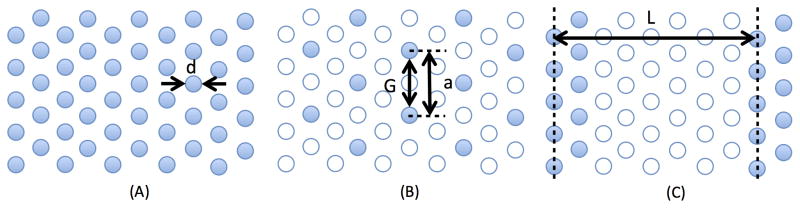
Schematic view of hexagonal (A and B) and lamellar (C) post arrays. The filled circles are the positions of the posts. The particular arrays (B) and (C) are created by removing posts from (A), as indicated by the open circles. Note here (B) and (C) have the same number of posts per unit area. The post diameter (d), the lattice constant for the hexagonal array (a), the gap between the posts (G), and the lamellar spacing (L) are indicated in the figure.

Brownian dynamics simulations are an ideal approach to address the role of the lattice structure on DNA separations in a post array. While there exists experimental resolution data in various hexagonal [4, 5, 7–12] arrays and one lamellar configuration [6], it is challenging to compare the results of different experiments [13] because the post diameters, device materials, DNA molecular weight, and the degree of optimization of the experimental protocols vary between different experiments. In our simulations, we fix the post diameter at 1 μm, which is in the range of post sizes used in the aforementioned experiments, and systematically vary the density of the arrays and their arrangement in silico for 7 different arrays (Supporting Information Fig. A1). Inasmuch as we have shown previously [14] that the model quantitatively agrees with experimental data at the single molecule level for systems similar to the ones we study here, we expect that our simulation results should provide reasonable estimates of the trends we would expect to observe in experiments.

2 Materials and Methods

2.1 Brownian dynamics simulations

We used a Brownian dynamics simulation of a bead-spring Rouse model in an inhomogeneous electric field. The model has been described elsewhere [15], and a brief recapitulation of the method is provided in the Supporting Information. We simulated two DNA molecular weights: λ-DNA (48,500 base pairs, 37 beads) and 1.5λ-DNA (55 beads). Before applying the electric field, we first relaxed both DNA for 10⁵ time steps in free solution using a time step δt = 2×10⁻⁴. Then we placed the relaxed DNA into the post array and used an additional 10⁵ time steps for further relaxation prior to applying the electric field. We will report all of our results in dimensional form by converting lengths with the maximum spring length (0.58 μm), time with the bead diffusion time (20 ms), and electric fields via the Péclet number (Pe = 1 corresponds to 16 V/cm). The conversion from dimensionless to dimensional quantities appeared previously [15, 16]. The ensemble for a given combination of the electric field, DNA size, and post array consists of 96 different initial configurations, where each simulation proceeds until the center-of-mass of the DNA reaches a distance L_c = 2.01 mm.

The model is parameterized to match the properties of λ-DNA, and thus has the correct diffusion coefficient for that molecular weight. Since the model does not include hydrodynamic interactions, the resulting diffusivity of 1.5λ-DNA is approximately 85% of the predicted Zimm diffusivity. This is likely an overestimate of the error in the diffusion coefficient for since these molecular weights are partially draining [17, 18]. In any event, we do not expect the underestimate of the diffusivity for 1.5λ-DNA to be a significant issue since it is similar to the experimental error in the λ-DNA diffusivity used to parameterize the model [19]. Moreover, during the free solution motion, the convective force is strong at the chain length scale when compared to diffusion, and during the hooking event, the chain is stretched and hydrodynamic interactions are weak [20]. While hydrodynamic interactions would quantitatively change the results, it seems unlikely that they would affect the key conclusions, and the increased computational cost for confined systems with hydrodynamic interactions [21] does not justify the potential benefits.

Figure 1 shows the geometric parameters describing the post arrays. The posts have a diameter d = 1 μm, the post array is contained within a slit of depth of 4.5 μm, and the electric field is applied such that the DNA motion is from left-to-right in the figure. For the hexagonal arrays, as illustrated in Fig. 1B, we define the gap between the edges of neighboring posts as G = a − d, where a is the lattice constant for the hexagonal array. We simulated gap sizes of 1 μm, 2 μm and 3 μm. These arrays are given the nomenclature GxHex, where x = (1,2,3) refers to the gap size. For the lamellar arrays, such as the one illustrated in Fig. 1C, we define each lamella as two rows of posts separated by a region of post-free space. Following the experimental approach used for the nanofence [6], we also use the minimum gap size from the hexagonal arrays, G = 1 μm, and lamellar periods of L = 10 μm, 20 μm and 40 μm. These arrays are denoted as G1Ly, where y = (10, 20, 40). We also simulated the particular system in Fig. 1C, where L corresponds to 8 rows of a hexagonal array. The system in Fig. 1C, denoted G1L8R (i.e., y = 8 Rows), has the same density of posts as the G3Hex array in Fig. 1B. This approach permits a simple control for the post arrangement at fixed post density. For clarity, we provide schematics of all 7 arrays to scale in Supporting Information Fig. A1. These arrays are spatially periodic, so the electric field distributions therein are obtained with the same methods we used previously [15].

2.2 Separation Resolution

The simulations furnish the distribution of times, t, for the DNA in the ensemble to reach the finish line at L_c. We can compute the resolution from

$$R_s=\frac{{\overline{t}}_{1.5\lambda }-{\overline{t}}_{\lambda }}{2({\sigma }_{\lambda }+{\sigma }_{1.5\lambda })}$$ (1)

where t̄ and σ are the mean and the standard deviation of the arrival times for each species at the finish line. For visualization purposes, we have also created histograms of the arrival times using 10 bins of equal temporal width.

2.3 Number of Collisions and Holdup Time

The collisions are identified by the plateaus in the center-of-mass trajectory versus time and the holdup time is computed from the offset of the constant velocity trajectories before and after the collisions, following the standard approach [22]. For a given trajectory i, we compute the total number of collisions, n_i, and the average holdup time, τ_i, during the transit to the finish line. Our plots of the number of collisions and holdup time correspond to the average and standard deviation of the distributions for n_i and τ_i over the i = 1:96 members of the ensemble.

Since we fix the total distance traveled during the simulation at L_c, different arrays contain a different number of posts. To arrive at a quantity that captures the efficiency of the array, we have also computed the number of collisions “per lamella.” The hexagonal arrays can be treated as a small lamellar spacing $L=\sqrt{3}a$.

2.4 Radius of gyration and survival probabilities

To understand the dynamics between collisions, we computed the instantaneous radius of gyration as a function of the distance since the previous collision, R_g(x-x₀), where x is the current location of the DNA molecule and x₀ is the location of the preceding collision. For a given molecule and a given collision, we track the radius of gyration until the subsequent collision. Since the instantaneous R_g data are intrinsically noisy, we bin the data into regularly spaced bins of x_j ± 0.5 μm, where x_j is the center of the j^th bin corresponding to a given value of R_g(x_j). A given simulation of 96 molecules over 2 mm contains a large number of collisions; for example, we observed 19479 collisions in G1Hex at 8 V/cm. As the distance x-x₀ increases, the DNA should relax and eventually reach a plateau value of R_g. At the same time, as the distance increases, DNA make subsequent collisions and drop out of the ensemble used to compute R_g(x-x₀). Returning to our example with G1Hex at 8 V/cm, the number of trajectories still in the ensemble drops to 5680 at x-x₀ = 10 μm. If we let N(x-x₀) be the number of measurements still in the ensemble at position x-x₀, then the ratio N(x-x₀)/ N(0) can be interpreted as the survival probability for the first-time passage process to the adsorbing “boundary condition” corresponding to the next collision. When the survival probability is close to unity, the number of trajectories in the ensemble is large, so the data are smooth. For small survival probabilities, the number of trajectories can become small, which makes the R_g data noisy.

3 Results and Discussion

3.1 Hexagonal arrays

Inasmuch as the separation in a post array arises from the collisions with the obstacles, it seems logical to increase the post density, so long as the density is not so high that the dynamics cross over into biased reptation with orientation [1]. We speculate that this logic has driven the impressive engineering required for dense nanofabricated post arrays [5, 8, 9, 12]. Remarkably, our simulation data in Figs. 2 and 3 do not support this logic. Rather, the resolution increases as the gap size changes from 1 μm to 2 μm, and then decreases upon a further increase of the gap size to 3 μm. Keep in mind that we are testing the basic hypothesis about array density, not the resolution of particular nanofabricated devices; the bead-spring model encounters discretization errors when the post sizes or the gaps become close to the maximum spring length (0.58 μm). Figure 3 includes data for electric fields of 8 V/cm and 16 V/cm. As the resolution is clearly superior at the lower electric field, our subsequent analysis will focus primarily on the 8 V/cm case.

Figure 2.

Histogram of the finish time for ensembles (each consisting of 96 molecules) of λ-DNA (hatched with 45 degree diagonals) and 1.5λ-DNA (open bars) in 4 different post arrays at 8 V/cm. The y-axis refers to the number of molecules in each bin.

Figure 3.

Separation resolution between λ-DNA and 1.5λ-DNA for 7 different post array geometries at 8 V/cm (dark bars) and 16 V/cm (light bars). The fractions above each dark bar are the numerator and denominator from Eq. (1).

Figure 4 explains the resolution trend at 8 V/cm. As expected, Fig. 4A shows that the densest array leads to the most collisions. However, it is important to note that both the λ-DNA and 1.5λ-DNA exhibit almost the same number of collisions in the densest array. Here, the half-gap between the posts (0.5 μm) is smaller than the radius of gyration measured inside this array during the equilibration step prior to applying the electric field (0.69 μm for λ-DNA and 0.82 μm for 1.5λ-DNA). As a result, neither of these molecules can completely relax into a coil inside the array. After partial relaxation, their collisional cross-section to the next post is effectively the size of the gap between posts, independent of molecular weight. In contrast, when we move to a less dense array, both sizes of DNA can now relax inside the array. The number of collisions for the 1.5λ-DNA then becomes larger than that for λ-DNA due to the difference in their radii of gyration. However, Fig. 4C shows that the difference in the holdup times is essentially independent of the post array size. Inasmuch as the retardation inside the array increases as the product of the number of collisions and holdup time increases, we can attribute the increase in the resolution as we move from a gap of 1 μm to 2 μm, in part, to an increase in the distance between the peaks; the difference in the number of collisions for the two DNA serves as a weighting factor to accentuate the difference in their holdup times.

Figure 4.

The number of collisions and holdup time for λ-DNA (hatched with diagonal lines) and 1.5λ-DNA (hatched with cross lines) in hexagonal post arrays (left column) and lamellar post arrays (right column) at 8 V/cm. The lamellar case G1L8R is included in both columns to provide a comparison with the equal density hexagonal array G3Hex. The bar height represents the mean value of the ensemble (containing 96 molecules), while the error bar shows the corresponding standard deviation.

As the gap size increases further to 3 μm, Fig. 4C shows that the number of collisions decreases by almost 4-fold compared to the 1 μm gap. In this very sparse array, the DNA spend much of their time meandering through the empty space between the posts at their free solution mobility. This so-called channeling effect was first described in simulations for sparse arrays in uniform electric fields [23, 24]. Although the channeling effect is suppressed by the curved field lines present in experimental systems and our simulation model [25], it must begin to occur even in electrically insulating systems as the array becomes sufficiently dilute [10]. This qualitative explanation is supported by the data in Fig. 4B, which shows that the “efficiency” of the 3 μm gap device is lower than its denser counterparts. Although the 3 μm gap array still exhibits the same molecular-weight trends for the number of collisions and the holdup time difference as the 2 μm gap array, the resolution decays for the larger gap size because the time spent in collisions is becoming small compared to the time moving at the free solution mobility.

These observations about the number of collisions and holdup time are reflected in the various contributions to the resolution, which are included as the numerator and denominator of Eq. (1) in Fig. 3 for the 8 V/cm data. The biggest spacing between the peaks for the hexagonal array is observed for the 2 μm gap, owing to the DNA-size dependent number of collisions, whereas the relative effects of the number of collisions and their ability to retard the DNA as a function of molecular weight seem to cancel out when we compare the peak spacing in the 1 μm and 3 μm arrays. The denominator, which corresponds to the band broadening, decreases monotonically with the gap size. The band broadening arises from the product of the dispersion coefficient and the residence time in the array. The dispersion coefficient is governed by fluctuations in the number of collisions and the holdup time [26]; an inspection of Fig. 4 indicates that these quantities are relatively insensitive to the gap between the posts. However, it is readily apparent from Fig. 2 that the DNA spend a longer time reaching the finish line as the array density increases. Thus, the increase in the band broadening as the density of the array increases is attributable primarily to the lower electrophoretic mobility, not the differences in the rate of band broadening.

The overall trends at 8 V/cm appear to be replicated in the data at 16 V/cm in Fig. 3, albeit with a lower resolution. Inasmuch as both the electrophoretic velocity and the dispersivity scale linearly with the electric field [27], these scaling laws imply that distance between the peaks scales inversely with electric field and the peak widths are independent of the electric field. As a result, the lower resolution at a higher electric field and a fixed elution distance L_c is expected.

3.2 Lamellar arrays

In a recent experimental paper [6], we proposed that arranging the posts into a lamellar structure would be an improvement over a hexagonal array, since it should permit relaxation of the DNA and increase the efficiency of the collisions. The posts used in the experimental system had 500 nm diameters, hence the moniker “nanofence” array. Since we are focusing here on micron-sized posts, it is more appropriate to refer to this system as a lamellar structure.

One of the challenges in testing a claim of a “better” array is to provide a reasonable basis for comparison. We felt that an appropriate approach is to compare the separation resolution between a hexagonal array (G3Hex) and a lamellar array (G1L8R) with the same post density, which we illustrated in Fig. 1. The superiority of the lamellar array (G1L8R) for this particular post density and molecular weights is apparent in Fig. 2, with two easily resolvable peaks eluting in the lamellar lattice. As we see in Fig. 3, the origin of the improved resolution is the markedly better spacing between the peaks at the expense of a slight increase in the band broadening, which is consistent with experiments [6]. The improved efficiency of the lamellar structure is also apparent in Fig. 4. Figure 4A shows that the number of collisions in the lamellar lattice increases compared to the equivalent hexagonal system, with the molecular-weight dependence of the number of collisions also increasing. Figure 4C shows that the difference in the holdup times is also much larger in the lamellar system when compared to the hexagonal system since the DNA are able to relax between each collision (which we will discuss more thoroughly in Section 3.3). Both of these observations are consistent with an improvement in the peak spacing; the product of the number of collisions and their duration is a much stronger function of molecular weight in the lamellar system than in the equivalent hexagonal system.

It is also worth noting that, although there is space between the lamella for the DNA to relax to their free solution coils, the number of collisions per lamella for the lamellar systems in Fig. 4E is not unity. This observation is again consistent with experimental data [6].

Although we endeavored to create a hexagonal post array and a lamellar post array with the same density for an “apples-to-apples” comparison, it is evident from Fig. 3 that the resolution of this lamellar array exceeds the resolution of all of the hexagonal post arrays that we studied. This result refutes the conventional wisdom that more collisions leads to better separations, as Fig. 4A shows that the number of collisions in the lamellar array is roughly half that in the most dense array. Indeed, we drew Fig. 1 in such a manner to make it clear that this particular lamellar system (G1L8R) can be constructed from the densest hexagonal array (G1Hex) by deleting 75% of the posts in the latter array.

Inasmuch as there is a non-monotonic dependence of the resolution on the post spacing in the hexagonal system, it is natural to wonder whether a similar trend exists for the lamellar spacing as well. Figure 3 indicates that the resolution is indeed non-monotonic. The origin of the increase in resolution as L increases in the lamellar array is the same as that when G increases in the hexagonal array: the densest lamellar array, like its hexagonal counterpart, does not allow the DNA to relax sufficiently between collisions. The reason for the decrease in the resolution as L increases even further is somewhat different than in the hexagonal array. While Fig. 4E shows that the efficiency per lamella increases with the lamellar spacing, consistent with increased relaxation between lamella as their distance increases, the number of collisions before the finish line and the separation resolution are smallest for the largest lamellar spacing. The decay in resolution at the larger spacing occurs in both the hexagonal and lamellar systems due to a loss of collisions before reaching the finish line. However, the reason for the reduction in the number of collisions differs. In the hexagonal system, the DNA needs to diffuse to align itself with field lines that drive it into the post [25]. In the lamellar system, the DNA needs to be convected from lamella to lamella.

The basic principles underlying the separation resolution at 8 V/cm also apply at 16 V/cm. As we see in Fig. 3, the maximum in the separation resolution at 16 V/cm has shifted to a larger lamellar spacing of roughly double that at 8 V/cm. (With the limited number of arrays, it is impossible to be more precise about the location of the resolution maximum.) This is expected if the resolution maximum occurs for a lamellar spacing where the DNA have enough time to relax before the next collision without “wasting” time being convected to the next lamella in the relaxed conformation. Since the velocity in the empty region of the lamella is proportional to the electric field, we would expect to require twice the distance at 16 V/cm to achieve the same extent of relaxation as at 8 V/cm.

3.3 Relaxation and survival probability

One of the most interesting features of the lamellar systems is the number of collisions per lamella (Fig. 4E). For the smaller λ-DNA, the number of collisions per lamella seems to be relatively insensitive to the lamellar spacing, whereas this value increases monotonically with lamellar spacing for the larger 1.5λ-DNA. To investigate this phenomenon further, Figs. 5 and 6 plot both the radius of gyration and the survival probability for these molecules as a function of distance from the previous collision. For λ-DNA, the relaxation is almost complete before the DNA reaches the shortest lamellar period at 10 μm. As a result, the probability of colliding in a given lamella is a constant at approximately 45%, independent of the lamellar spacing. The survival probability is thus a discrete version of an exponential decay [26]. In contrast, the relaxation of 1.5λ-DNA requires more than 10 μm at 8 V/cm. As a result, the number of collisions increases for 1.5λ-DNA as the lamellar period increases.

Figure 5.

The radius of gyration R_g as a function of migration distance since the previous collision (top panel) and survival probability (bottom panel) for λ-DNA in 4 different post arrays at 8 V/cm.

Figure 6.

The radius of gyration R_g as a function of migration distance since the previous collision (top panel) and survival probability (bottom panel) for 1.5λ-DNA in 4 different post arrays at 8 V/cm.

The radius of gyration data in Figs. 5 and 6 also explain why the collision probability is not unity in the lamellar systems. Consider the case where L = 10 μm. The radius of gyration data exhibit periodic “bumps” that correspond to the location of the lamella. This behavior results from deformation of the DNA that does not lead to a collision. (Recall that any DNA that collides is removed from the ensemble for these plots.) The DNA are impacted when passing through a lamella, but the deformation is not always sufficient to lead to a collision. Experiments in the nanofence [6] produced similar behavior, where the DNA were observed occasionally to slither through the nanofence without a collision.

For comparison, we have also included the results for a hexagonal array in Figs. 5 and 6. The survival probability decays exponentially, in agreement with experimental data for a hexagonal post array [14] and the assumption made in continuous-time random walk models [26].

It is also worth noting that the plateau values for the radius of gyration in the hexagonal array in Figs. 5 and 6 are not only larger than the plateau values in lamellar systems, but also considerably larger than the values obtained during the equilibration inside the array prior to the electrophoresis (0.69 μm for λ-DNA and 0.82 μm for 1.5λ-DNA) due to survivorship bias. Recall that the R_g data in Figs. 5 and 6 correspond to those DNA molecules that have not yet made their next collision at a distance x – x₀ since the previous collision. For the dense G1Hex array, we thus conclude that those DNA that translate the longest distances between collisions are still somewhat extended and slithering through the lattice.

4 Conclusions

Our systematic comparison of hexagonal and lamellar post array lattices leads to two key conclusions. First, for a hexagonal lattice, a sparse post array seems to be superior to a dense post array, a speculation that we had made previously [25] without the support provided by the present work. Second, lamellar structures like the nanofence array [6] seem to be superior to a hexagonal post array at the equivalent density of posts, although we have only proven this point for a single case here. However, since the best lamellar post array outperforms all of the hexagonal post arrays in our study, it seems reasonable to speculate that there is an optimal lamellar design for a given molecular weight range. However, one certainly needs to be careful with the design of the array with respect to the relaxation times of the DNA and their radii of gyration for a more complicated mixture. If the array is too dilute, then the advantages of a sparse hexagonal array or a lamellar structure are lost. This point raises some challenges for designing arrays for separating a large range of molecular weights, since the span of length and time scales for the DNA will also be large. However, this problem arises in all microfabricated separation devices [1], and even in gel electrophoresis [28], especially with respect to band inversion phenomena [29–31].

We posit that our study here is an appropriate comparison of these different types of systems, since the simulations trivially control for various aspects (e.g., uniformity and magnitude of the electroosmotic flow) that are difficult to control in experiments. Moreover, we have made the comparisons at the same electric field with the same DNA molecular weights, which is difficult to do with the experimental data available in the literature. However, our recent review of the literature [13] indicates that the best separations have been obtained in dense nanopost arrays, seemingly in contrast to the predictions here. One possibility is that there is something special about the collision with a nanopost relative to a micropost. However, isolated post experiments with different post sizes [32] do not support this conclusion, provided that the posts are smaller than the radius of gyration of the DNA. (Naturally, nanoposts are required for separating shorter, but still flexible, DNA molecules.) We suspect that the higher resolutions in nanopost experiments result from better experimental protocols rather than some intrinsic but unrecognized advantage of a dense nanopost array. Recall that the separation resolution results from many factors, and we have only examined the in-array effects here. In particular, sharp injections are pre-requisites for an effective microfluidic separation [33], but the details of the injection protocols vary widely between experiments [5, 10, 12]. Our results suggest that it would be worthwhile to compare dense nanopost arrays directly to sparse arrays and nanofences using identical hard materials, buffers, wall coatings, injection protocols, and DNA solutions. The multichannel approach used previously to compare ordered and disordered systems [34] is a particularly attractive option since it isolates the in-array differences while minimizing experimental artifacts.

References

- 1.Dorfman KD. Rev Mod Phys. 2010;82:2903–2947. [Google Scholar]
- 2.Volkmuth WD, Duke T, Wu MC, Austin RH, Szabo A. Phys Rev Lett. 1994;72:2117–2120. doi: 10.1103/PhysRevLett.72.2117. [DOI] [PubMed] [Google Scholar]
- 3.Nixon GI, Slater GW. Phys Rev E. 1994;50:5033–5038. doi: 10.1103/physreve.50.5033. [DOI] [PubMed] [Google Scholar]
- 4.Doyle PS, Bibette J, Bancaud A, Viovy JL. Science. 2002;295:2237. doi: 10.1126/science.1068420. [DOI] [PubMed] [Google Scholar]
- 5.Kaji N, Tezuka Y, Takamura Y, Ueda M, Nishimoto T, Nakanishi H, Horiike Y, Baba Y. Anal Chem. 2004;76:15–22. doi: 10.1021/ac030303m. [DOI] [PubMed] [Google Scholar]
- 6.Park SG, Olson DW, Dorfman KD. Lab Chip. 2012;12:1463–1470. doi: 10.1039/c2lc00016d. [DOI] [PMC free article] [PubMed] [Google Scholar]
- 7.Minc N, Fütterer C, Dorfman KD, Bancaud A, Gosse C, Goubault C, Viovy JL. Anal Chem. 2004;76:3770–3776. doi: 10.1021/ac035246b. [DOI] [PubMed] [Google Scholar]
- 8.Chan YC, Lee YK, Zohar Y. J Micromech Microeng. 2006;16:699–707. [Google Scholar]
- 9.Shi J, Fang AP, Malaquin L, Pépin A, Decanini D, Viovy JL, Chen Y. Appl Phys Lett. 2007;91:153114. [Google Scholar]
- 10.Ou J, Carpenter SJ, Dorfman KD. Biomicrofluidics. 2010;4:013203. doi: 10.1063/1.3283903. [DOI] [PMC free article] [PubMed] [Google Scholar]
- 11.Ou J, Joswiak MN, Carpenter SJ, Dorfman KD. J Vac Sci Technol A. 2011;29:011025. [Google Scholar]
- 12.Yasui T, Kaji N, Okamoto Y, Tokeshi M, Horiike Y, Baba Y. Microfluid Nanofluid. 2013;14:961–967. [Google Scholar]
- 13.Dorfman KD, King SB, Olson DW, Thomas JDP, Tree DR. Chem Rev. 2013;113:2584–2667. doi: 10.1021/cr3002142. [DOI] [PMC free article] [PubMed] [Google Scholar]
- 14.Olson DW, Ou J, Tian M, Dorfman KD. Electrophoresis. 2011;32:573–580. doi: 10.1002/elps.201000466. [DOI] [PubMed] [Google Scholar]
- 15.Cho J, Dorfman KD. J Chromatogr A. 2010;1217:5522–5528. doi: 10.1016/j.chroma.2010.06.057. [DOI] [PubMed] [Google Scholar]
- 16.Chen Z, Dorfman KD. Phys Rev E. 2013;87:012723. doi: 10.1103/PhysRevE.87.012723. [DOI] [PMC free article] [PubMed] [Google Scholar]
- 17.Mansfield ML, Douglas JF. Soft Matter. 2013;9:8914–8922. [Google Scholar]
- 18.Tree DR, Muralidhar A, Doyle PS, Dorfman KD. Macromolecules. doi: 10.1021/ma401507f. (in press) [DOI] [PMC free article] [PubMed] [Google Scholar]
- 19.Smith DE, Perkins TT, Chu S. Macromolecules. 1996;29:1372–1373. [Google Scholar]
- 20.André P, Long D, Ajdari A. Eur Phys J B. 1998;4:307–312. [Google Scholar]
- 21.Graham MD. Annu Rev Fluid Mech. 2011;43:273–298. [Google Scholar]
- 22.Saville PM, Sevick EM. Macromolecules. 1999;32:892–899. [Google Scholar]
- 23.Patel PD, Shaqfeh ESG. J Chem Phys. 2003;118:2941–2951. [Google Scholar]
- 24.Mohan A, Doyle PS. Phys Rev E. 2007;76:040903(R). doi: 10.1103/PhysRevE.76.040903. [DOI] [PubMed] [Google Scholar]
- 25.Ou J, Cho J, Olson DW, Dorfman KD. Phys Rev E. 2009;79:061904. doi: 10.1103/PhysRevE.79.061904. [DOI] [PubMed] [Google Scholar]
- 26.Minc N, Viovy JL, Dorfman KD. Phys Rev Lett. 2005;94:198105. doi: 10.1103/PhysRevLett.94.198105. [DOI] [PubMed] [Google Scholar]
- 27.Dorfman KD, Viovy JL. Phys Rev E. 2004;69:011901. doi: 10.1103/PhysRevE.69.011901. [DOI] [PubMed] [Google Scholar]
- 28.Viovy JL. Rev Mod Phys. 2000;72:813–872. [Google Scholar]
- 29.Noolandi J, Rousseau J, Slater GW, Turmel C, Lalande M. Phys Rev Lett. 1987;58:2428–2431. doi: 10.1103/PhysRevLett.58.2428. [DOI] [PubMed] [Google Scholar]
- 30.Doi M, Kobayashi T, Makino Y, Ogawa M, Slater GW, Noolandi J. Phys Rev Lett. 1988;61:1893–1896. doi: 10.1103/PhysRevLett.61.1893. [DOI] [PubMed] [Google Scholar]
- 31.Heller C, Pohl F. Nucleic Acids Res. 1989;17:5989–6003. doi: 10.1093/nar/17.15.5989. [DOI] [PMC free article] [PubMed] [Google Scholar]
- 32.Joswiak MN, Ou J, Dorfman KD. Electrophoresis. 2012;33:1013–1020. doi: 10.1002/elps.201100471. [DOI] [PubMed] [Google Scholar]
- 33.Manz A, Harrison DJ, Verpoorte EMJ, Fettinger JC, Paulus A, Lüdi H, Widmer HM. J Chromatogr A. 1992;593:253–258. [Google Scholar]
- 34.Olson DW, Dorfman KD. Phys Rev E. 2012;86:041909. doi: 10.1103/PhysRevE.86.041909. [DOI] [PubMed] [Google Scholar]
Associated Data
This section collects any data citations, data availability statements, or supplementary materials included in this article.