Cost Savings Effects of Olanzapine as Long Term Treatment for Bipolar Disorder

Abstract

Newer and more expensive drugs account for most of the recent rapid growth of spending on prescription drugs in the past nine years. But if more expensive drugs can reduce the use of other types of health care services, total health care costs might fall. In this paper, I investigate the “drug-offset” hypothesis for an atypical antipsychotic drug, olanzapine, compared to lithium, to treat bipolar disorder. I use a propensity-score method to match on observed variables. Then, using various identification strategies, namely interrupted time series, differencing strategies, and an instrument-variable approach, I find that olanzapine does not reduce spending on other types of medical care services, compared with lithium. Olanzapine users spend $330 per month more than lithium users on non-drug health care services after drug treatment and $470 more per month on total health care spending, contradicting the “drug-offset” hypothesis in this case.

JEL classification: H51; I1; I18; C1; C2

1. Introduction

Concomitant with a rise in total health care spending, there has been a disproportionately large increase in prescription drug spending. Research has found that switching to newer and highly-priced drugs accounts for one-third of this rapid growth (Kaiser_Family_Foundation 2005). In response to the rapid rise in drug spending, both public and private programs have established pharmaceutical-related cost containment policies, using various mechanisms to reduce the use of newer and more expensive drugs. However, the growing reliance on newer and higher-priced drugs is not necessarily driving the rise in total health care spending. The use of newer prescription drugs may result in lower use of other types of care, such as reduced inpatient admissions or outpatient visits. If so, savings from using a newer drug may offset the incremental increase in drug costs while achieving the same level of health outcome (often called a “drug offset” effect).

I examine the “drug offset” effect for one condition, bipolar disorder, which is associated with a high rate of hospitalization. Primary treatment for bipolar disorder involves the use of mood stabilizers, which have proven to be very effective. I will examine the offset effect by comparing two drugs, lithium, a traditional mood stabilizer, and olanzapine, a new atypical antipsychotic alternative to treat bipolar disorder. There is some clinical evidence that olanzapine is more effective than lithium in preventing relapses to mania, and olanzapine users are associated with lower discontinued treatment because of side effects, compared to lithium users. Therefore I hypothesize new olanzapine users spend less on other types of medical services after drug treatment, compared with new lithium users, provided that their prior health status is similar.

To estimate this effect, I use insurance claims and enrollment data from MarketScan databases between 1998 and 2001. I construct the initial sample by selecting the 13,746 individuals diagnosed with bipolar disorder within the study period. Then I identify new users of the drugs of interest who were continuously enrolled in the health plans one year prior to and one year after they started to use drugs. This sample design enables me to assess changes in non-drug services before and after the drug therapy. The central challenge for a reliable estimation is that drug treatments are not randomly assigned among patients with bipolar disorder. As a result, I use the propensity-score method to match lithium users with olanzapine users to ensure the two groups are comparable in observed variables such as previous health status, demographic characteristics, and health insurance plan types.

Potential unobserved population heterogeneity, however, remains a main obstacle to unbiased causal estimates. In attempt to gauge the robustness of the results, I use three estimation strategies: (1) interrupted time series; (2) differencing strategies with various specifications and assumptions for variance-covariance structures; and (3) an instrument-variable strategy. None of these methods can completely eliminate the endogeneity problem, but they can serve as checks for robustness.

Overall, the findings presented in this paper imply that patients taking the newer and more expensive drug do not save on non-drug health care services, compared to those who take the older and less expensive drug. This does not support the hypothesis that newer prescription drugs show a “drug-offset” effect.

The paper proceeds as follows. In the next section, I discuss the clinical effectiveness of comparison medications to treat bipolar disorder and previous studies on “drug-offset” effects. Section 3 summarizes the empirical challenges and estimation strategies used in the paper. Section 4 describes the data, sample selection and key variables, followed by two sections on model specifications and results. Section 7 contains discussion and conclusions.

2. Background and literature reviews

2.1. Bipolar disorder and its treatment

Bipolar disorder, also known as manic-depressive illness, is a brain disorder that causes unusual shifts in a person's moods, energy, and ability to function. It affects 2.3 million adult Americans, about 0.8 percent of the population. Patients' moods swing from depths of depression to intense highs of mania. In depressive episodes, patients experience desperate hopelessness, cannot think, talk, move or care, and often feel no point of living. In manic episodes, patients are irritable, angry, frightened, uncontrollable, and their thoughts are often overwhelmingly confused. The primary treatment for bipolar disorder is mood-stabilizer medication. Left untreated, bipolar patients' moods shift from one extreme to another, so the disease is associated with a high rate of hospitalization.

The traditional mood stabilizer, lithium, has been the main treatment of bipolar disorder for both acute and maintenance care. Since late 1990's, atypical antipsychotics, especially olanzapine, have been prescribed to treat acute manic or mixed bipolar episodes. There is evidence that olanzapine is better than lithium to prevent relapses to mania, and olanzapine is generally better tolerated and more convenient to take than lithium. But olanzapine is at least ten times more expensive than lithium.¹

Following the Food and Drug Administration's (FDA) approval of olanzapine as an acute treatment of bipolar disorder in March 2000, American Psychiatric Association guidelines (2002) added olanzapine as a monotherapy alterative for less ill patients. The guidelines also stated that providers may consider using olanzapine for maintenance therapy, despite the absence of clinical trials confirming its clinical advantages over lithium. Olanzapine was approved as a maintenance therapy to treat bipolar disorder in February 2004, based on a few clinical trials indicating its superior effectiveness over placebo.

2.2. Previous studies

The effectiveness of olanzapine as an acute or a maintenance treatment compared to placebo is well established (Bowden, Lecrubier et al. 2000; Vieta, Reinares et al. 2001; Tohen, Chengappa et al. 2002; Namjoshi, Risser et al. 2004; Tohen, Chengappa et al. 2004; Vieta, Calabrese et al. 2004; Bowden 2005; Muzina and Calabrese 2005; Tohen, Greil et al. 2005; Vieta and Goikolea 2005).However, the evidence that olanzapine is superior to lithium is inconclusive. Tohen et al. (Tohen, Greil et al. 2005) compared the effectiveness of olanzapine and lithium by following 400 patients with bipolar I disorder² for one year. They found that the rate of manic recurrence did not differ significantly between patients taking lithium and those taking olanzapine for the first 150 days of the trial, but thereafter the rate was significantly lower for the olanzapine group. Depression relapse rates did not differ significantly. Bridle et al. (Bridle, Palmer et al. 2004) ran a meta analysis of studies from clinical trials and economic evaluations in the electronic databases maintained by the National Institute for Clinical Excellence. They did not find significant differences between olanzapine and lithium in terms of effectiveness.

Literature on the so-called “drug offset” effect is sparse. A recent study by Duggan (Duggan 2005) sheds some light on different estimation strategies to evaluate the impact of a new drug class on other types of health services compared to an older drug class. Duggan used a sample of Medicaid recipients from the state of California for the 1993-2001 period to investigate the relationship between the use of atypical antipsychotics and other health care services. He used three different identification strategies to demonstrate a consistent result: Medicaid spending on atypical antipsychotics increased 610% during the study period, but the shift to new drug treatments did not reduce spending on other types of medical care.

An alternative approach is from societal perspective, represented by a series of studies by Lichtenberg (Lichtenberg 1996; Lichtenberg 2001). Using the 1996 Medical Expenditure Panel Survey (MEPS) data, he found on average that replacing a 15-year old drug with a 5.5-year old drug will increase drug spending by $18, but reduce other medical spending by $72, to achieve the same or better health outcome. Using the same dataset and focusing on cardiovascular drugs, Miller and his colleagues (Miller, Moeller et al. 2006) found that Lichtenberg's findings are sensitive to two key confounders, the number of drugs used and the mix of drugs of different ages.

The Lichtenberg study assumed the same “drug-offset” effects across disease conditions and drug classes, and did not address the endogeneity problem due to patient-unrelated omitted variables. The main goal of the Miller et al. study is to document the association between drug age and non-drug spending, not a causal relationship. The Duggan study assumed the same “drug-offset” effects on other types of medical care spending, without distinguishing new users from switchers, and acute drug therapy from maintenance drug therapy.

In this paper, I will conduct a retrospective study to compare the effectiveness of olanzapine and lithium as maintenance treatment for bipolar I disorder by examining their impact on the use of other health care services. The current study contributes to the drug-offset effect literature in three ways. First, I select my study sample based on clinically-sound inclusion and exclusion criteria. To mitigate the complication due to switching drugs and the interaction among drugs, I selected patients who initiated drugs of interest during the study period (new users) and were on the drugs for at least three months after initiation. I excluded patients who were ever diagnosed schizophrenia, as the primary treatment for schizophrenia is also atypical antipsychotics. Second, I compare various methodologies to obtain consistent results. Specifically, I use a population-level interrupted time series method as well as individual-level empirical models including differencing strategies and an instrumental-variable approach to mitigate the endogeneity problem in the choice of drug treatment. Third, this study contributes to incremental cost-effectiveness analysis of olanzapine and lithium to treat patients with bipolar disorder.

3. Estimation Strategies

Using insurance claims and enrollment data, I conduct a quasi-experimental study, with repeated measures before and after intervention for two groups of patients diagnosed with bipolar disorder: olanzapine users as the treatment group and lithium users as the control group. The intervention is drug therapy, with the onset event defined as the day drug use was initiated. Outcomes are repeatedly measured for the periods twelve months prior to and twelve months after the onset events for each individual in the sample.

Investigating the effect of new prescription drugs on other types of health care expenditures is difficult given that drug treatment is not randomly assigned. Individuals who take a certain drug are likely to differ from their counterparts who do not, in both observed and unobserved factors. I use a propensity-score method to mitigate the heterogeneity in treatment choice caused by observed variables. To reduce biases introduced by both incomplete matching and inexact matching, I match the treatment group to the control group observations based on a propensity score using “greedy matching” techniques (Parsons 2002). After matching, the treatment group and the control group are comparable in all observed variables that are included in the estimation models.

Potential population heterogeneity in unobserved variables, however, could exist after propensity-score matching, leading to biased estimates. In an attempt to gauge the robustness of the results, I use three quasi-experimental strategies: (1) an interrupted time series model; (2) differencing strategies with various specifications and assumptions for error covariance structures; and (3) an instrumental variable strategy. None of these methods can entirely eliminate the endogeneity problem, but they can serve as checks for the robustness of the estimates.

I start with an interrupted time series approach to estimate whether non-drug expenditures after the initiation of drug treatment differ between olanzapine users and lithium users. Data are collected for twenty-four time points (months), twelve months before and twelve months following the initiation of drug therapy. The interrupted period contains two months: the month when patients experienced crisis (e.g. being hospitalized) immediately before drug treatment and the month when patients initiated drug therapy of interest. This time-series design with comparison group allows me to control for previous trends in the outcome and to evaluate longitudinal effects of the drug treatment. As a population-level estimate strategy, however, interrupted time series cannot control for individual-level characteristics that might affect the outcome variables. This problem motivates me to use several individual-level estimate approaches as discussed below.

The first individual-level estimation approach is a differencing strategy by comparing the change in non-drug spending after and before drug treatment between olanzapine and lithium users. Differencing strategy takes advantages of time repeated measures within individuals to mitigate the endogeneity problem caused by individual-specific and time-unvarying factors, especially unobserved variables that are not controlled by propensity score matching. ³

Differencing strategies cannot mitigate the unobserved, patient-unrelated heterogeneity, nor can they address heterogeneity due to time-varying characteristics. For example, physician practice patterns simultaneously affect patients' choice of drugs and other types of health care services. If an old physician is more likely to prescribe old drugs and more likely to refer patients to inpatient care services, then we will observe a correlation between the use of an old drug and higher spending in inpatient care services. If patients change their providers over time, then the endogeneity problem due to physician practice pattern cannot be mitigated by the differencing strategy. This motivates my third strategy – an instrumental variable approach. The instrumental variable approach can solve the endogeneity problem due to omitted variables, measurement errors or simultaneous causality. A valid instrumental variable should be highly correlated with the choice of drug therapy, but not correlated with omitted variables that might affect the use of other types of health care services. The time when a drug is approved by the FDA is not correlated with physician prescribing behaviors or other unobserved variables that might affect patients' spending on non-drug health care services. However, the FDA's approval of a drug will affect the choice of drug treatment. Thus, we can use an instrument of a dummy variable equal to one if the drug (either olanzapine or lithium) was initiated after the olanzapine approval date and zero otherwise. Two-stage-least-squares will be used to estimate the effect of a drug choice on the difference in non-drug spending before and after drug treatment.

I will discuss these empirical strategies in detailed specification forms in section 5. In the next section, I will describe the dataset and sample used for this study.

4. Data description and sample design

4.1. Data description

I analyze the MarketScan data for the 1998-2001 period. The annual MarketScan database collects private-sector health data from approximately 200 nationally-representative payers and is made up of three databases including benefit plan design database, commercial claims and encounter database, and Medicare supplemental database. In this study, only the first two databases are used. The benefit plan design database includes benefit plan types and service coverage information. The commercial claims and encounter database includes inpatient and outpatient claims, pharmacy claims, detailed patient information, and enrollment tables. The inpatient admission information includes data on principal procedures, diagnosis, and payments to facilities and physicians. The outpatient services information includes encounters and claims for services that were provided in a doctor's office, a hospital outpatient facility, an emergency room or other outpatient facility. The pharmacy claims data contains information on national drug codes (NDC, a code to identify prescription drugs), dosage forms, days of supply, prescription fill dates and payment types such as copayment, deductible and total gross payment.

4.2. Sample selection

In selecting the study sample, I included individuals who: (1) had a maintenance drug treatment, defined as continuous use of either olanzapine or lithium for at least three months within the 1998-2001 period; (2) were continuously enrolled in the network one year prior to and one year following the onset of drug treatment; (3) were diagnosed as bipolar disorder I,⁴ which is defined as having at least one inpatient diagnosis or two outpatient diagnoses during the two-year continuous enrollment period; and (4) had not used any atypical antipsychotics or any bipolar disorder related prescription drugs within six months prior to the onset day. I excluded individuals who had a diagnosis of schizophrenia, which is defined as having at least one inpatient diagnosis or two outpatient diagnosis during the two-year period. I initially identified 13,736 patients who had used either olanzapine or lithium for at least three months in the study period. Of these, 4677 of them were continuously enrolled one year prior to and one year following the onset of drug treatment. 1304 patients had taken both lithium and olanzapine for at least three months, and 3073 patients had a monotherapy of either lithium or olanzapine. After excluding patients who were diagnosed with schizophrenia, I obtain a sample of 1372 patients with bipolar disorder.⁵ Finally, I exclude those patients who had taken any atypical antipsychotic or bipolar disorder related drugs six months before the onset day. This leaves a final sample of 935 patients with a drug monotherapy, of which 221 are olanzapine users and 714 are lithium users.

4.3. Propensity score one-to-one matching

Ideally, the sample should include patients who take olanzapine and patients who take lithium that are identical except for the drug treatment. I first examine whether the two groups are comparable with respect to observed characteristics such as age, sex, geographic region, and medical spending prior to drug treatment. The comparison of patient characteristics⁶ shows that olanzapine users and lithium users are similar with respect to some observed demographic characteristics, including sex, likelihood of living in certain geographic regions and likelihood of having certain types of insurance. There are significant differences between two groups on other measures. Specifically, Health Maintenance Organization (HMO) enrollees are more likely to use lithium than olanzapine. Preferred Provider Organization (PPO) enrollees are more likely to use olanzapine than lithium, as are Non-Capitated Point-of-Service (POSNOCAP) enrollees. Furthermore, the frequency of being hospitalized for various reasons within a year before maintenance drug therapy was significantly higher for olanzapine users than lithium users. I found that 26% of olanzapine users were hospitalized before they initiated drug therapy, while only 12% of lithium users were. In addition, previous non-drug utilization and spending for mental health related services is significantly higher among olanzapine users than lithium users. ⁷The average number of major diagnosis codes in the year before drug treatment was six for olanzapine users and five for lithium users.

This comparison implies that the two drug groups are not comparable without further adjustment. Therefore, I use propensity scores to match olanzapine users with lithium users. I first estimate the probability of being an olanzapine user based on patients' demographic variables (age, sex and region), health insurance type and patients' health status (measured by the number of health service visits and indicators of major conditions in the year before drug treatment). Then, I use this probability as a benchmark to match the closest individual within the lithium group to a member of the olanzapine group. The propensity-score matching results in 212 lithium users matched with 212 olanzapine users.

The comparison table of patients' characteristics for the matched sample is reported in Table 1. After matching, the two groups are well balanced with respect to all the observed covariates in the period before drug treatment. This sample of 212 lithium users and 212 olanzapine users will be the sample of analysis throughout my study.

Table 1.

Descriptive Statistical Summary by User Group (Matched sample: 212 Olanzapine users and 212 Lithium users)

CHARACTERISTICS	OLANZAPINE	LITHIUM	P–Value
FEMALE	54.028	58.019	0.408
NORTHEAST	28.910	32.547	0.418
NORTHCEN	27.962	24.528	0.422
WEST	1.896	2.830	0.527
SOUTH	31.754	34.906	0.492
FFS	33.175	32.547	0.891
HMO	5.213	5.660	0.839
POSNOCAP	13.744	11.792	0.548
POSCAP	31.754	27.830	0.378
PPO	16.114	22.170	0.113
AGE	39(17)	40(15)	0.364
COUNTMDC1	6(3)	6(3)	0.430
ABUSE1	1(6)	0(3)	0.505
EPILEP1	0(1)	0(0)	0.133
HEART1	0(1)	0(3)	0.616
DIAB1	1(4)	1(4)	0.481
THERAPY1	7(12)	7(11)	0.962
NUMBD1	12(16)	13(14)	0.647
NUMMH1	20(19)	20(18)	0.862
NUMBDIP1	0(1)	0(1)	0.756
NUMBDOP1	12(16)	13(14)	0.658
NUMMHIP1	0(1)	0(1)	0.603
NUMMHOP1	19(19)	19(18)	0.882
SUMBD1	2,448(4,228)	2,721(5,284)	0.558
SUMBDIP1	1,343(3,383)	1,713(4,880)	0.365
SUMBDOP1	1,105(2,134)	1,008(1,549)	0.594
SUMMH1	3,922(5,606)	3,430(5,836)	0.377
SUMMHIP1	2,127(4,413)	1,919(5,050)	0.653
SUMMHOP1	1,795(2,799)	1,511(1,878)	0.220
SUMCL1	7,410(8,959)	7,216(9,178)	0.826
PROPENSITY SCORE	0.272(0.112)	0.270(0.110)	0.843

Notes:

(1) Postfix “1” stands for one-year before drug treatment and “2” stands for one-year after drug treatment. Suffix “sum” denotes non-drug spending and “num” denotes the number of claims. “bd” stands for bipolar disorder, “mh” stands for mental health, and “cl” stands for any medical services. “ip” is inpatient care and “op” is outpatient care. For example, sumbdip2 stands for total non-drug spending in bipolar disorder related inpatient services during the year after drug treatment.

(2) First few rows in the table are demographic variables, sex, enrollment region, health insurance type and age.

(3) Next are some indicators for medical conditions, “countmdc1” measures the number of major diagnostic codes. “Heart1” indicates number of incidents related to heart disease the patient ever had before starting drug treatment, likewise, for epilepsy (EPILEP1), substance abuse (ABUSE1), and diabetes (DIABETES1). “Therapy1” stands for the number of psychology therapies before a patient initiates drug treatment.

(4) High s.d. demonstrates high volatility in mental health spending. s.d. measures the variability of data around the mean, which is square root of sample variance, and s.e. measures how well this sample mean estimates population mean.

(5) Same notes apply for table 2

4.4. Outcome variables and explanatory variable

The outcome variables are non-drug spending in three levels of related services: total medical services, mental health services, and bipolar disorder related services.

The key explanatory variable is a dummy indicator that equals to one for olanzapine users as the treatment group and zero for lithium users as a comparison group.

The covariates included patients' demographic variables, health status indicators, and treatment patterns. Patients' demographic variables are sex, age categories (less than 17, 18-34, 35-44, 45-54, 55-64; the omitted category is less than 17, and there are no elderly in the sample), plan types (HMO, PPO with capitation or without capitation, FFS, and POS), and enrollment region (northeast, north-central, west, and south). Patients' previous health status is measured by health expenditures one-year prior to drug treatment, the number of inpatient care visits and outpatient care visits, the number of psychology therapies, the number of major diagnosis categories, and the number of incidents for the following conditions: heart disease, epilepsy (345.0-345.9⁸), substance abuse (304, 305), alcoholic psychoses (291.0-291.9) and diabetes (250). Drug treatment patterns include dosage and the length of drug treatment. Clinical evidence of olanzapine's effectiveness is well established for medium and high dosages (5mg, 10mg, and above), but not for a low dosage of 2.5mg. In order to control for the different effects due to different dosage levels, I create an indicator to identify patients who only took the low dosage form of olanzapine and control for it in the regression.

5. Model specifications

Before I investigate the relationship between the use of prescription drugs and non-drug spending using econometric strategies, I start with a simple time trend analysis. I use a sample of all patients who were diagnosed with bipolar disorder in the 1998-2001 period. There were substantial changes in the pharmacological treatment of bipolar disorder during this time, as shown in Figures A-1 and A-2 in the Appendix. Two trends should be noted. First, the proportion of olanzapine users among bipolar patients increased and the proportion of lithium users decreased during the study period. Second, the use of olanzapine increased faster after the FDA approved it to treat bipolar disorder in March 2000 (represented by a vertical line in the figures). The increase in the use of olanzapine and the decline in the use of lithium provide an opportunity to gauge the effect of drug choice on the outcome variables of interest. If the use of olanzapine reduces the demand for inpatient and other health care services more than lithium does, I should expect to see a decline in the non-drug spending on bipolar disorder related services and mental health related services during the same period. On the contrary, Figure A-3 in the Appendix indicates no noticeable decline in monthly non-drug spending on bipolar disorder related services and mental health related services in the period of 1998-2001.

However, the absence of an observed decline in spending on non-drug events could be explained by two possible complications. First, the majority of patients might be only on olanzapine for a few days. Second, the proportion of olanzapine users among patients with bipolar disorder is relatively small, only accounting for 10 percent of all users. These possibilities confirm why a carefully-conducted study design is warranted. As such, for the following estimation approaches, I focus on the matched sample of 212 olanzapine users and 212 lithium users.

5.1. Interrupted time series analysis

Figures 1 through 3 demonstrate the time trend of monthly-average non-drug spending in three levels of related services: total medical services, mental health, and bipolar disorder related services, respectively. The x-axis indicates month in time, equal to 1 to 24, with the drug initiation occurring at the thirteenth month. Each point on the jagged line in the figure indicates monthly-average non-drug spending for either the lithium users or olanzapine users (labeled in the figures). The straight lines in the figures are the predicted regression lines estimated by an interrupted time-series model.

Figure 1.

Monthly Non-drug Spending on Total Medical Services¹⁸

Figure 3.

Monthly Non-drug Spending on Bipolar Disorder Related Services

Two points are immediately observable: (1) average non-drug spending is the highest in the month immediately before the drug initiation; (2) average non-drug spending of olanzapine users is higher than that of lithium users after patients started the medication treatment, and this difference remains over time for both mental health and bipolar disorder related services but shrinks for total medical services.

The first observation implies that there is a significant increase in the use of inpatient care in the days leading up to an individual's first prescription for the drugs of interest. Patients perhaps experienced a crisis or other events that led to high service utilization; as a result, they may have received inpatient care or emergency room services before they initiated drug therapy. For the year after drug initiation, patients' service use was stabilized (i.e., no spikes were observed) . This stabilization results in reduced non-drug expenditures compared to the period immediately before drug initiation.

The second observation implies that olanzapine users did not spend less on non-drug events compared to lithium users. Thus, there is evidence against the hypothesis that the new treatment substantially lowered non-drug spending. To estimate numerical effects, I use an interrupted time series model.

The unit of observation is the person-month, with twelve points before and twelve points after drug initiation for each individual. For each person-month, there are 424 observations (212 lithium users and 212 olanzapine users). To estimate the interrupted time series model, I compute average health care expenditures for each group for each time point and estimate the effect of drug treatment, excluding an interrupted duration. The interrupted duration contains two person-months, the month when patients experienced crisis immediately before drug initiation and the month they initiated drug use (Wagner, Soumerai et al. 2002). The model specification is presented in equation (1).

$$\begin{array}{cc}\hfill & Y_t={\beta }_0+{\beta }_1{\mathit{treatment}}_t+{\beta }_2{\mathit{month}}_t+{\beta }_3{\mathit{post}}_t+{\beta }_4{\mathit{postmonth}}_t+\hfill \\ \hfill & {\beta }_5{{\mathit{treatment}}_t}^{\ast }{\mathit{month}}_t+{\beta }_6{{\mathit{treatment}}_t}^{\ast }{\mathit{post}}_t+{\beta }_7{{\mathit{treatment}}_t}^{\ast }{\mathit{postmonth}}_t+{\mathit{error}}_t\hfill \end{array}$$ (1)

Where,

Treatment is a dummy variable that equals 1 for olanzapine users and 0 for lithium users. Month measures time in months from the start of the study period; it ranges from to 1 to 24. Post is an indicator for time t occurring after intervention.

Postmonth measures the numbers of months after the intervention. It is coded 0 for all months before intervention, and equals to 1 to 12 for months after intervention.

The remaining variables are interaction terms between treatment and time series variables. Based on the definitions above, β₀ estimates the average monthly expenditures of lithium users for the baseline point (i.e., twelve months before they initiated lithium). β₁ estimates the difference in average monthly expenditures between olanzapine users and lithium users at the baseline point. β₂ estimates the incremental change by month in the average expenditure of lithium users before intervention, i.e., the baseline trend. β₃ estimates the change in the monthly-average expenditures for lithium users immediately after the intervention. β₄ estimates the incremental change in the trend in the monthly-average expenditures after intervention. The interaction terms estimate the incremental difference between olanzapine users and lithium users in each time series variable. For example, β₆ estimates the difference between olanzapine users and lithium users in the change in non-drug spending after and before drug treatment. This is essentially a difference-in-difference estimate.

Autocorrelation is detected through a plot of raw residuals against time. In the model, I adjusted for serial autocorrelation, and the Durbin-Watson statistic for the final regression model is close to 2, indicating the model is adjusted for autocorrelation. Throughout the analysis, I use maximum likelihood methods to estimate the effects, starting with a full model including all interaction terms as shown in equation (1), then using a stepwise method to estimate reduced models with the exclusion of insignificant interaction terms, and eventually reaching the most parsimonious model which only includes significant terms besides the main treatment.

Time series analysis estimates the effect of treatment at the population level, which does not control for individual characteristics. Thus, I will also estimate the effect of drug treatment after controlling for individual observables by using two individual-level estimate approaches, namely, differencing and instrumental-variable strategies.

5.2. Differencing strategies – individual-level estimates

One challenge with individual-level estimates comes from some unique characteristics associated with health care expenditure data: (a) a nontrivial fraction of zero outcomes in the sample, and (b) a positively skewed empirical distribution of the nonzero realizations. Normally, to address a big fraction of zero outcomes in expenditure data, a two-part model is required. Such a model consists of first estimating the probability of encountering a positive outcome and second estimating the impact of the intervention on the outcome conditional on a positive outcome. In this study, the unit of observation is person-month⁹, so only a small fraction of outcome expenditures are zero. Thus, a two-part model is not necessary. Instead, I adjust for the small share of zero outcomes in the data by adding a small positive number to zero outcomes.

However, the analysis still faces the problem of expenditures being highly positively skewed and heavily tailed (skewness=11; kurtosis=186). To address this issue, a power transformation is required. The literature has suggested three classes of models to address the high skewness of health care expenditure data: least-squares (LS) estimators for the ln(y) with retransformation, the generalized linear models (GLM) with log link function and gamma distribution, and generalized Gamma model (Duan 1991; Manning 1998; Manning and Mullahy 2001; Manning, Basu et al. 2005). The LS-based methods can be biased in the face of heteroscedasticity if not appropriately retransformed (Duan 1991; Manning 1998; Manning and Mullahy 2001; Manning, Basu et al. 2005). Heteroscedasticity is detected across all time trend related variables in my sample, which makes an appropriate retransformation challenging. Due to this heteroscedasticity, without adjustment, generalized Gamma model also yields biased estimates. The GLM method can yield consistent yet possibly imprecise estimates if the log-scale error is heavy-tailed. Following the algorithm suggested by Manning and Mullahy (Manning 1998; Manning and Mullahy 2001), and after considering the tradeoff between bias and precision, I choose to use GLM with a gamma distribution and a log link function. Box-Cox test detects that logarithm transformation fits the data well. A modified Park test determines the mean-variance relationship and leads to the conclusion that a gamma distribution assumption fits the data appropriately.¹⁰

The repeated measures within individuals provide an opportunity to difference out individual-specific and time-unvarying omitted variables that may cause the endogeneity problem. However, panel data estimation requires an assumption of an appropriate variance-covariance structure across repeated observations on individuals. I test four structures, specifically, (a) Huber/White robust variance adjusted by patient clusters, (b) a patient fixed-effect generalized linear model, (c) a generalized estimation equation to fit population-averaged panel-data model, and (d) a generalized linear mixed model to allow random correlation effects across time within individuals. All four models assume a log link function for a power transformation of the outcome variable and a gamma distribution for the mean-variance relationship.¹¹ The outcome variable is total non-drug medical spending.

Below are model specifications with various assumptions about variance-covariance structures. (a) Generalized linear model with gamma distribution and log link function adjusted by patient clusters

$$\begin{array}{cc}\hfill & \ln \left(E(Y_{\mathit{it}}\mid X)\right)={\beta }_0+{\beta }_1{\mathit{treatment}}_{\mathit{it}}+{\beta }_{2\mathit{it}}\mathit{month}+{\beta }_3{\mathit{post}}_{\mathit{it}}+\hfill \\ \hfill & {\beta }_4{\mathit{postmonth}}_{\mathit{it}}+{\beta }_5{{\mathit{treatment}}_{\mathit{it}}}^{\ast }{\mathit{post}}_{\mathit{it}}+\sum _{k=6}^K{\beta }_k{X}_{k,i}\hfill \end{array}$$ (2)

Or

$$E(Y\mid X)=\exp \left(X\beta \right)=\mu (X;\beta )$$

The central structure of this model is an exponential conditional mean or log link relationship as above. The mean-variance relationship follows a gamma distribution with the structure of v(y|x) = κ(μ(x))² , where k>0; that is, the standard deviation is proportional to the mean. Huber/White robust estimates of variance are used.

(b) Patient fixed-effect generalized linear model

$$\begin{array}{cc}\hfill & \ln \left(E(Y_{\mathit{it}}\mid X)\right)={\beta }_0+{\beta }_1{\mathit{month}}_{\mathit{it}}+{\beta }_2{\mathit{treatment}}_{\mathit{it}}+{\beta }_3{\mathit{post}}_{\mathit{it}}+\hfill \\ \hfill & {\beta }_4{\mathit{postmonth}}_{\mathit{it}}+{\beta }_5{{\mathit{treatment}}_{\mathit{it}}}^{\ast }{\mathit{post}}_{\mathit{it}}+c_i\hfill \end{array}$$ (3)

Availability of panel data allows me to consistently estimate the average treatment effect without assuming the ignorability of treatment, provided the treatment varies over time and is uncorrelated with time-varying unobserved variables that affect the response. If the treatment effect is constant over time and assumed to have the same effect for each patient, then patient fixed effects consistently estimate the treatment effect. Fixed effect analysis assumes E(c_i | x_i) to be any function of x_i . This allows me to consistently estimate partial effects in the presence of time-constant omitted variables that can be arbitrarily related to the observables x_i . Thus, it is robust but comes at a price: time-constant factors in x_i cannot be included in the model. Also, fixed effects analysis assumes the same effect of drug therapy on non-drug expenditure for different individuals. Therefore, I will also consider a model that allows drug effects to differ among individuals, such as an approach that estimates a population-average treatment effect.

(c) Generalized estimation equation to fit a population-average panel-data model This approach uses generalized method of moments to estimate β. The key features of such estimation approaches are the moment:

$$S\left(\beta \right)=\sum _{i=1}^K{D}_i^{\prime }{V}_i^{-1}(Y_i-{\mu }_i\left(\beta \right))=0$$ (4)

Where

$$\begin{array}{cc}\hfill D_i& =\frac{\partial {\mu }_i}{\partial \beta }\hfill \\ \hfill {\mu }_{\mathit{it}}& =\exp \left({x_{\mathit{it}}}^{\prime }\beta \right)\hfill \end{array}$$

Unstructured working correlation is assumed to be:

$$\mathit{corr}(Y_{\mathit{it}},Y_{\mathit{is}})=\{\begin{array}{cc}1\hfill & t=s\hfill \\ {\alpha }_{\mathit{ts}}\hfill & t\ne s\hfill \end{array}\phantom{\}},\text{where}{\widehat{\alpha }}_{\mathit{ts}}=\frac{1}{(K-p)\varphi }\sum _{i=1}^K{e}_{\mathit{it}}{e}_{\mathit{is}}$$

Where p is the number of parameters in the regression model. The dispersion parameter ϕ is estimated by

$$\widehat{\varphi }=\frac{1}{(N-p)}\sum _{i=1}^K\sum _t^{T_i}{e}_{\mathit{it}}^2,\text{where}N=\sum _{i=1}^K{T}_i$$

(d) Generalized linear mixed model A generalized linear mixed model allows a random correlation effect across time on individuals. The mixed model consists of two parts: the parameters of the mean model are referred to as fixed-effects parameters, and the parameters of the variance-covariance model are referred to as covariance parameters.

The fixed-effects parameters are associated with known explanatory variables, estimated by β_k in equation (5). In this study, repeated measurements are taken over time for each individual, so repeated measurements are correlated or exhibit variability that changes. I assume two-level random-effect parameters that impact the variability of the data. One level is spending at baseline of lithium users (intercept) and the second level is month-to-month change within individual (measured by b_t ). The model specification is:.

$$\begin{array}{cc}\hfill & \ln \left(E(Y_{\mathit{it}}\mid X,b_t)\right)=b_t+b_t{\mathit{month}}_{\mathit{it}}+{\beta }_1{\mathit{treatment}}_{\mathit{it}}++{\beta }_2{\mathit{post}}_{\mathit{it}}+\hfill \\ \hfill & {\beta }_3{\mathit{postmonth}}_{\mathit{it}}+{\beta }_4{{\mathit{treatment}}_{\mathit{it}}}^{\ast }{\mathit{post}}_{\mathit{it}}+{\beta }_5{{\mathit{treatment}}_{\mathit{it}}}^{\ast }{\mathit{postmonth}}_{\mathit{it}}+\sum _{k=6}^K{\beta }_k{X}_{k,\mathit{it}}\hfill \end{array}$$ (5)

Where

• Y_it is total non-drug medical expenditures of patient i in month t;

• b_t is a random effect across time within individuals. It allows different variances for the intercept and the slope of the time trend and a covariance matrix between them. This captures the autocorrelation across months within each patient.

• β_k is a vector of fixed effects of covariates.

• X_{k ,it} is a set of covariates measured on patient i at month t, including patients' demographic variables, health status variables and treatment pattern variables as discussed above.

5.3. Instrumental variables

Differencing strategies can consistently estimate partial effects in the presence of time-constant omitted variables that are correlated with key explanatory variables, but differencing strategies cannot address the endogeneity problem caused by time-varying or patient-unrelated unobserved factors that might affect outcome variables. For example, if a doctor is more likely to prescribe olanzapine and to refer patients to inpatient care, then we would observe an association between higher non-drug expenditures and use of olanzapine. This problem cannot be solved by differencing strategies if patients' relationships with physicians vary over time. Therefore, an appropriate instrumental variable is needed to mitigate the endogeneity problem caused by both observed and unobserved omitted variables.

A good instrument meets two conditions: (1) the instrument should be highly correlated with the independent variables of interest, i.e., choice of drug therapy; and (2) the instrument should not be correlated with omitted variables that might affect the outcome variable. The date when the FDA approved olanzapine to treat bipolar disorder is not correlated with physician behavior patterns or other unobservables that might affect patients' non-drug medical expenditures but will affect the choice of drug treatment. After olanzapine (Zyprexa) was approved in March 2000 to treat acute bipolar disorder, the number of new users of olanzapine significantly increased, both for acute treatment and maintenance treatment.¹² This trend suggests a potential instrumental variable, namely, whether or not patients initiated a drug therapy after March 2000. A dummy variable is created that equals one if the patient initiated the drug (either olanzapine or lithium) after March 2000 (which I refer to as “new” patients) and zero otherwise (which I refer to as “old” patients). The first-stage F-test is 14.8, indicating a strong correlation between the instrument and the explanatory variable.

The exogeneity of an instrumental variable is difficult to test. In the matched sample, all observed variables are well balanced between the new patient and old patient groups, as reported in Table 2. In addition, the descriptive summary split by the indicator of instrument for the unmatched sample (including 219 olanzapine users and 689 lithium users) is reported in Table A-3 in the Appendix. The two groups are well balanced for most critical observables such as previous health spending, health care utilization, indicators of severe conditions (i.e., heart disease, diabetes, epilepsy, substance abuse), and demographic variables such as gender and enrollee regions. However, new patients (i.e., patients who initiated the drug after March 2000) are four years younger than old patients on average. New patients are more likely to be in HMO plans and less likely to be in FFS plans compared with old patients. This difference implies an expansion of HMO plans from 1998 to 2001. Moreover, the average number of psychological therapy visits before drug treatment is one third higher for new patients compared with old patients. I assume a conditional exogeneity of the instrumental variable by controlling for the abovementioned unbalanced factors in the two-stage least squares model as shown in equation (6).

Table 2.

Descriptive Statistical Summary by Instrument Variable (Matched Sample: 212 Olanzapine users and 212 Lithium users)

CHARACTERISTICS	After March 00	Before March 00	P–Value
FEMALE	55.414	56.391	0.845
NORTHEAST	31.210	30.451	0.870
NORTHCEN	29.299	24.436	0.272
WEST	3.822	1.504	0.130
SOUTH	28.025	36.466	0.075
FFS	26.115	36.842	0.023
HMO	7.006	4.511	0.274
POSNOCAP	15.924	10.902	0.135
POSCAP	31.210	28.947	0.623
PPO	19.745	18.797	0.811
USERID	63.694	41.729	< 0.0001
AGE	38(17)	41(15)	0.174
COUNTMDC1	6(3)	6(3)	0.190
ABUSE1	1(4)	1(5)	0.664
EPILEP1	0(1)	0(0)	0.325
HEART1	0(2)	0(3)	0.655
DIAB1	1(4)	1(4)	0.969
THERAPY1	8(11)	6(12)	0.201
NUMBD1	10(14)	14(16)	0.0062
NUMMH1	20(20)	20(18)	0.945
NUMBDIP1	0(1)	0(1)	0.281
NUMBDOP1	10(14)	14(16)	0.0048
NUMMHIP1	1(1)	0(1)	0.053
NUMMHOP1	19(19)	19(18)	0.868
SUMBD1	2,544(5,135)	2,609(4,572)	0.897
SUMBDIP1	1,832(4,676)	1,349(3,889)	0.277
SUMBDOP1	712(1,158)	1,260(2,150)	0.0007
SUMMH1	4,012(6,211)	3,477(5,413)	0.371
SUMMHIP1	2,567(5,351)	1,702(4,315)	0.086
SUMMHOP1	1,445(1,731)	1,776(2,691)	0.125
SUMCL1	7,704(8,591)	7,082(9,333)	0.487
PROPENSITY SCORE	0.282(0.114)	0.265(0.109)	0.119

Two-stage least squares model:

$$\begin{array}{cc}\hfill & {\mathit{treatment}}_i={\beta }_0+{\beta }_1{\mathit{fdaiv}}_i+\sum _{k=2}^K{\beta }_k\mathit{Co}\mathrm{var}{\mathit{iates}}_i+{\mathit{error}}_i\hfill \\ \hfill & \ln Y_{i,\mathit{pst}}-\ln Y_{i,\mathit{pre}}={\pi }_0+{\pi }_1\mathit{tre}\widehat{a}{\mathit{tment}}_i+\sum _{k=2}^K{\pi }_k\mathit{Co}\mathrm{var}{\mathit{iates}}_i+{\mathit{error}}_i\hfill \end{array}$$ (6)

In the first stage, I estimate how much the instrument explains the variation of the choice of drugs, controlling for gender, age, patients' previous health utilization, health insurance type, and enrollee region. In the second stage, I use the predicted linear probability of being an olanzapine user from the first stage as the key explanatory variable to estimate the effect of drug treatment on non-drug spending. The unit of observation is the person-year. As discussed previous, the original outcome variable (expenditures in dollars) was positively skewed but the natural logarithm of the outcome variable follows a normal distribution; therefore, the natural logarithm transformation is used. This log-difference linear model estimates how the choice of drug affects the ratio between the yearly average non-drug expenditures before and after drug treatment. If the before-after ratio is less than one, it implies a reduction on non-drug expenditures after the drug treatment, and vice versa. π₁ estimates the ratio of this ratio between olanzapine and lithium users $\left(i.e.,\frac{Y_{\mathit{after}}∕Y_{\mathit{before}}\mid \mathit{olanzapine}}{Y_{\mathit{after}}∕Y_{\mathit{before}}\mid \mathit{lithium}}\right)$. Provided that the baseline non-drug expenditures are same for both drug groups, π₁ measures how much more olanzapine users spent in non-drug expenditures compared with lithium users.

6. Results

6.1. Interrupted time series

Results estimated by the interrupted time series are reported in Table 3. Three columns show the results in three levels of outcome expenditures: non-drug total medical expenditures, non-drug expenditures in mental-health related services and non-drug expenditures in bipolar disorder related services, respectively.

Table 3.

Interrupted Time Series Regression Model to Estimate the Impact of the Drug Treatment on Monthly Non-drug Spending

	Total Medical Services	Mental Health Services	Bipolar Disorder Services
A. Full segmented regression
INTERCEPT	393.907** (4.419)	165.953** (3.014)	144.286** (3.519)
TREATMENT	−40.589 (−0.324)	45.322 (0.583)	−39.247 (−0.683)
MONTH	22.106 (1.651)	8.851 (1.077)	4.899 (0.794)
POST	−451.006** (−3.417)	−186.714** (−2.260)	−129.937** (−2.156)
POST MONTHLY CHANGE	16.069 (0.842)	7.627 (0.654)	7.134 (0.809)
TREATMENT*MONTH	1.583 (0.084)	−5.087 (−0.438)	1.357 (0.156)
TREATMENT*POST	664.288** (3.588)	264.064** (2.273)	96.994 (1.149)
TREATMENT*POST MONTHLY CHANGE	−52.239 (−1.894)	−4.742 (−0.283)	3.253 (0.255)
B. Reduced segmented regression
INTERCEPT	389.180** (5.775)	183.516** (4.182)	139.146** (4.512)
TREATMENT	−31.084 (−0.580)	16.289 (0.452)	−31.351 (−1.290)
MONTH	22.887** (2.469)	6.014 (1.011)	5.758 (1.353)
POST	−455.104** (−3.792)	−135.517** (−2.063)	−150.451** (−3.293)
POST MONTHLY CHANGE	15.192 (0.970)	5.434 (0.651)	8.459 (1.416)
TREATMENT*POST	672.952** (4.476)	164.106** (3.237)	137.668** (4.071)
TREATMENT*POST MONTHLY CHANGE	−50.525** (−2.728)
C. Most parsimonious regression
INTERCEPT	360.116** (5.783)	167.668** (4.603)	173.848** (9.649)
TREATMENT	−29.773 (−0.533)	16.564 (0.454)	−31.074 (−1.223)
MONTH	27.981** (3.516)	8.719** (2.039)
POST	−414.876** (−3.576)	−132.785** (−2.008)	−115.715** (−2.902)
POST MONTHLY CHANGE			13.943** (3.159)
TREATMENT*POST	600.896** (4.450)	163.686** (3.190)	139.005** (3.928)
TREATMENT*POST MONTHLY CHANGE	−40.526** (−2.557)

Notes: Robust t-statistics are in parenthesis.

^*indicates significance at the 0.1 level,

^**indicates significance at the 0.05 level.

The full regression model includes all interaction terms between treatment and time-series variables. However, the full model might not fit the data best, since it forces the baseline trend, the before-after change, and the after-treatment monthly change to be different between olanzapine users and lithium users when in fact there is no significant difference between the two groups. Therefore, I use a stepwise elimination process to exclude non-significant interaction terms, until only significant terms are kept in the model. These results are reported in Section C in Table 3 as the most parsimonious segmented regression model. The discussion below focuses on these results in Section C.

a. Non-drug spending on total medical services

There is no significant difference in previous non-drug expenditures between the two drug groups. The baseline month-to-month change is $28 in the average non-drug spending for lithium users and similar for olanzapine users. After drug therapy, compared to the month before patients experienced crisis, the non-drug expenditures of lithium users decreases by $415, while the non-drug expenditures of olanzapine users increases by $156.¹³ The difference between the two drug groups in change in non-drug spending after and before drug treatment is therefore $571. But the difference-in-difference gap shrinks by $41 each month throughout the study period.¹⁴ At the end of the first year after drug therapy, the difference reduces to $125. When smoothed over the year, the average monthly difference-in-difference estimate is $328, which implies that olanzapine patients spent $328 more in monthly average non-drug medical services during the first year after drug therapy than lithium patients did. In addition, olanzapine costs $153 per month¹⁵ and lithium costs $16 per month. Factoring in the direct cost of the drugs, olanzapine users spend $465 more in total health care spending per month than lithium users.

b. Non-drug spending on mental health related services

Lithium users and olanzapine users are comparable in previous non-drug expenditures on mental health related services. On average, lithium users spent $168 in non-drug mental health services one year before they initiated drug therapy, and olanzapine users spent $16 more. Monthly spending increased by approximately $9 per month for both groups. Immediately after drug therapy, non-drug expenditures of lithium users decreased by $133, while non-drug expenditures of olanzapine users increased by $47. The difference between the two drug groups after and before drug treatment is $180. This difference remains the same during the entire year after drug initiation.

c. Non-drug spending on bipolar disorder related services

Lithium users and olanzapine users are also comparable in previous non-drug expenditures on bipolar disorder related services. After drug therapy, non-drug expenditures of lithium users decrease by $116, while non-drug expenditures of olanzapine users decrease by $8. The difference between the two drug groups after and before drug treatment is $108. There is no significant reduction in this gap within the first year after drug treatment.

Table 4 summarizes the above findings, disaggregated at the monthly level. The change in non-drug spending between the second month after drug initiation (month 13) and the month before crisis (month 11) differ between olanzapine users and lithium users. This change of olanzapine users is higher than the change encountered by lithium users across three levels of outcome: $531 more in non-drug medical services, $180 more in mental-health related non-drug services, and $108 more in bipolar-disorder related non-drug services. The difference in the latter two levels of non-drug spending between the two groups remains the same at the end of the first year after drug initiation, while the difference in non-drug total spending declined over time from $531 in the second month to $125 at the end of the year.

Table 4.

Interrupted Time Series Regression Model to Estimate the Monthly Impacts of Drug Treatment on Monthly Non-drug Spending During the First Year after Drug Therapy

Month	14	15	16	17	18	19	20	21	22	23	24
Total Medical
Lithium users	337	365	393	421	449	477	505	533	561	589	617
Olanzapine users	868	855	842	830	817	805	792	780	767	755	742
Difference	531	490	450	409	368	328	287	247	206	166	125
Ratio	2.57	2.34	2.14	1.97	1.82	1.69	1.57	1.46	1.37	1.28	1.20
Mental Health
Lithium users	157	166	174	183	192	201	209	218	227	235	244
Olanzapine users	337	346	355	363	372	381	390	398	407	416	424
Difference	180	180	180	180	180	180	180	180	180	180	180
Ratio	2.15	2.09	2.03	1.98	1.94	1.90	1.86	1.83	1.80	1.77	1.74
Bipolar Disorder
Lithium users	72	86	100	114	128	142	156	170	184	198	212
Olanzapine users	180	194	208	222	236	250	264	278	292	305	319
Difference	108	108	108	108	108	108	108	108	108	108	108
Ratio	2.50	2.25	2.08	1.95	1.84	1.76	1.69	1.64	1.59	1.55	1.51

6.2. Results from differencing strategies

The results from the generalized linear model with gamma distribution and log link function with a Huber-White robust variance are reported in Column 1 of Table 5. Among interaction terms, only the coefficient of the interaction between the treatment and post variables is significant. This implies that the change in non-drug expenditures after and before drug therapy differs between olanzapine users and lithium users. Olanzapine users spent more in non-drug expenditures after drug therapy, and the change in spending for olanzapine users was 1.64¹⁶ times larger than that of lithium users. For an average lithium user, non-drug expenditures in the month immediately after drug therapy were $414, versus $740 for an average olanzapine user in that month. This difference in non-drug expenditures remains the same throughout the first year after drug therapy. The results from the generalized linear model with patient fixed effects are shown in Column 2 of Table 5. The results are similar to those found in the generalized linear model adjusted by cluster of patient. After drug therapy, the change in non-drug expenditures for olanzapine users was 1.7 times higher than lithium users. For an average lithium user, this model estimates that the non-drug medical expenditure in the month immediately after drug therapy was $496, versus $852 for an olanzapine user. The difference of $356 in non-drug spending between drug groups remains throughout the first year after drug therapy.

Table 5.

Generalized Models to Estimate the Impact of Drug Treatments on Total Non-drug Spending

	(1)	(2)	(3)	(4)
	GLMGAMMA	FIXEDEFFECT	GEEPANEL	GLMIX
TREATMENT	1.060	1.117	1.120	1.006
	(0.39)	(0.15)	(0.78)	(0.05)
BASE MONTHLY TREND	1.012	1.006	1.013	1.043**
	(0.61)	(0.68)	(0.62)	(3.67)
POST	0.904	0.908	1.027	0.822
	(0.46)	(1.07)	(0.11)	(1.42)
POST MONTHLY CHANGE	0.987	0.982	0.974	0.938**
	(0.49)	(1.61)	(0.85)	(3.41)
POST TREATMENT LEVEL EFFECT	1.642*	1.536**	1.559*	1.747**
	(2.41)	(5.47)	(2.17)	(3.14)
AGE 18-34	0.944		0.748	0.786
	(0.27)		(1.32)	(1.40)
AGE 35-44	0.699*		0.625**	0.717*
	(2.09)		(2.58)	(2.26)
AGE 45-54	0.683*		0.637*	0.663**
	(2.14)		(2.44)	(2.75)
AGE 55-64	1.136		0.882	0.820
	(0.56)		(0.55)	(1.24)
AGE >=65	1.476		1.412	1.426
	(0.76)		(0.59)	(0.91)
FEMALE	1.077		1.193	1.136
	(0.62)		(1.44)	(1.30)
SOUTH	0.794		0.787	0.780*
	(1.88)		(1.94)	(2.53)
WEST	1.402		1.433	0.862
	(0.70)		(0.76)	(0.57)
FFS	1.257		1.206	1.434**
	(1.84)		(1.60)	(3.40)
HMO	1.055		0.939	1.152
	(0.24)		(0.31)	(0.77)
PRE # MAJOR DIAGNOSIS	1.136**		1.143**	1.219**
	(6.00)		(5.93)	(11.35)
PRE HEART DISEASE	1.065		1.054	1.055
	(1.02)		(0.96)	(1.21)
PRE DIABETES	1.016		1.023	1.013
	(1.38)		(1.66)	(1.21)
PRE # PSYCHOTHERAPY	1.016**		1.017**	1.022**
	(4.23)		(4.12)	(5.36)
PRE EPILEPSY	1.097		1.083	1.169
	(0.66)		(0.90)	(1.79)
MONTHS ON DRUG	0.999		1.005	1.002
	(0.16)		(0.92)	(0.66)
POST MONTHLY TREATMENT				0.972
				(1.24)
Observations	9366	9366	9366	9366
Number of patients	424	424	424	424

The results from the generalized estimation equation are reported in Column 3 of Table 5. In the second month after drug therapy, the average monthly non-drug medical expenditure was $446 for lithium users and $794 for olanzapine users. On average, the non-drug spending of olanzapine users after drug treatment is 1.73 times higher than that of lithium users. There is no significant change in this gap throughout the year after drug therapy.

The results from the generalized linear mixed model are shown in Column 4 of Table 5. For lithium users, non-drug expenditures increased 1.04 times each month in the year before they initiated drug treatment. In the month after drug therapy, the non-drug expenditure dropped to 0.82 times than in the month before. In the twelve months thereafter, the monthly non-drug expenditure decreased by 0.94 times each month. In contrast to lithium users, olanzapine users' non-drug expenditures were 1.44¹⁷ times higher in the month after drug treatment compared with the month before the patient had crisis. Starting from the eighth month after drug treatment, olanzapine users started to have a decline in non-drug expenditures. Therefore, the gap in non-drug expenditure after drug treatment between olanzapine users and lithium users decreased throughout the study period, but the decline was not significant. If not taking this insignificant monthly-decline effect into consideration, then non-drug expenditures for olanzapine users were 1.76 times higher than lithium users during the first year after drug treatment. In dollars, non-drug spending of olanzapine users was $338 higher than that of lithium users in the first month immediately after drug treatment, and the gap remained the same throughout the year.

Despite different assumptions of variance-covariance structures, the results from the four models are consistent. The difference in non-drug spending after and before drug treatment differs between olanzapine users and lithium users, and the difference between olanzapine users and lithium users ranges from $326-$356, with higher spending by olanzapine users.

6.3. Results from instrumental variables estimation

The results from the instrumental variables estimation are reported in Table 6. For an average lithium user, the ratio of yearly non-drug expenditures after and before drug treatment is 0.808. Lithium users spent less in non-drug expenditures in the year after initiating use of lithium. For an average olanzapine user, the yearly non-drug expenditure after drug treatment is 1.076 times higher than the month before patients experienced a crisis. Given that the baseline expenditures of the two drug groups are similar, the post non-drug expenditures of olanzapine users are 1.29 times higher than those of lithium users. Olanzapine users spent $209 more than lithium users in monthly non-drug medical spending after drug treatment. This result is consistent with previous estimates from differencing strategies, yet the magnitude is smaller. The smaller effect is due to the fact that the instrumental variable estimate applies only to the subgroup of patients whose choice of drug is affected by the approval of drugs. Patients who initiated olanzapine before the drug was approved might have more severe conditions than patients who initiated olanzapine after the approval, which could explain the smaller magnitude of the IV estimates.

Table 6.

Instrument Variable Regressions on the Impact of Drug Treatments on Total Non-drug Medical Spending

	(1)	(2)	(3)
	2SLS	2SLS–RATIO	FIRST–STAGE
TREATMENT	0.254	1.289
	(0.35)	(0.35)
FEMALE	−0.028	0.973	−0.021
	(0.19)	(0.19)	(0.43)
AGE 18–34	0.036	1.036	0.021
	(0.14)	(0.14)	(0.22)
AGE 35–44	0.087	1.091	−0.078
	(0.39)	(0.39)	(1.02)
AGE 45–54	−0.040	0.961	−0.018
	(0.20)	(0.20)	(0.23)
AGE 55–64	0.400	1.492	−0.024
	(1.33)	(1.33)	(0.27)
AGE >=65	0.451	1.569	0.145
	(0.74)	(0.74)	(0.66)
FFS	−0.266	0.767	−0.106
	(1.36)	(1.36)	(1.82)
HMO	−0.026	0.974	−0.283**
	(0.08)	(0.08)	(3.17)
PRE HEART DISEASE	−0.057	0.945	0.015
	(0.78)	(0.78)	(0.51)
PRE DIABETES	−0.009	0.991	−0.006
	(0.65)	(0.65)	(0.81)
PRE # PSYCHOLOGICAL THERAPY	−0.012*	0.988*	0.000
	(2.13)	(2.13)	(0.16)
PRE SUBSTANCE ABUSE	0.021*	1.021*	0.003
	(2.18)	(2.18)	(0.63)
PRE # MAJOR DIAGNOSIS CODES	−0.049	0.952	0.005
	(1.95)	(1.95)	(0.60)
NORTHEAST	−0.337	0.714	−0.089
	(1.51)	(1.51)	(1.27)
WEST	−0.693	0.500	−0.187
	(1.19)	(1.19)	(1.29)
SOUTH	−0.012	0.988	−0.102
	(0.06)	(0.06)	(1.71)
INSTRUMENT–POST FDA			0.192**
			(3.85)
Constant	0.330		0.561**
	(0.60)		(6.35)
Observations	424	424	424
R–squared	0.06	0.06	0.09
1st stage F–test			14.80
Prob > F			0.000

Note: Robust t statistics in parentheses

^*significant at 5%;

^**significant at 1%

6.4. Summary

Compared to lithium users, olanzapine users spent approximately $330 more in monthly average non-drug medical services during the first year after drug therapy. In particular, olanzapine users spent $180 more in monthly mental-health related non-drug services, and $108 more in monthly bipolar-disorder related non-drug services relative to lithium users. In addition, olanzapine costs $140 per month more than lithium does, and therefore olanzapine users spend $470 more in total health care spending per month than lithium users.

7. Conclusions

This study attempts to investigate “drug-offset” effefct for a specific condition. Using three empirical strategies, I consistently estimate that patients with bipolar disorder do not have lower non-drug spending after drug initiation by taking olanzapine rather than lithium. Patients who take olanzapine spend approximately $330 more per month in non-drug spending and $470 more per month in total health care spending, compared to patients taking lithium. This result is consistent with Duggan's recent study on drug-offset effects for the same drug agent using a sample of Medicaid beneficiaries to treat schizophrenia. The findings from this study do not support the hypothesis that new drugs may to some extent pay for themselves by reducing the need for other health care services. These results suggest several possibilities: (1) the higher price of olanzapine can not be justified by its superior pecuniary effectiveness; (2) patients are not able to perfectly judge health effects or not completely sensitive to price of health care services; and (3) payers might not have enough bargaining power to negotiate a drug price that can be justified by the level of effectiveness.

One limitation with this study is the small sample size. This study draws on valid clinical information by applying strict inclusion and exclusion eligibility criteria, and draws on attributes of quasi-experimental study design to mitigate the endogeneity problem. However, this study design is implemented with an expense of a large sample size, as the MarketScan dataset is not a typical longitudinal dataset that follows up same enrollees over time. Nevertheless, due to the random select mechanism used by Marketstat, the continuously enrolled patients are not systematically different from those who are not continuously enrolled. Therefore, only using continuously enrolled patients will not result in the external threat for the generalization of results.

What implications for policies do research on “drug-offset” effect hold? “Drug-offset” effects are studied from two perspectives: aggregate level and specific-condition level. Aggregate-level research on “drug-offset” has its merits in general policy making, especially in the face of the scarcity of evidence for specific drugs. If on average, newer drugs are associated with less use of other types of non-drug services, a policy that rewards new drugs rather than seeks to limit their use can reduce total health case costs, vice versus. Nevertheless, the evidence for a specific condition or category of prescription drugs can serve as extra information and therefore add values to make heterogeneous policies for specific medicines and subgroups. If an innovated medicine can prevent patients from being hospitalized, the private and public drug coverage programs should cover that medicine to minimize the overall health system cost. “Drug-offset” model assumes that patients are able to judge health effects and fully responsible for the payment for health care services, and they choose between prescription drug and non-drug services to minimize total health cost to achieve a certain level of health outcome. In reality, however, patients do not always have full information or incentives to choose the optimal drug. If patients are not able to judge health effects or not fully responsible for financial payments, they might choose more highly-priced prescription drugs that are not associated with higher benefits. This results in a social cost with a loss for plans or payers without generating gains for patients. Therefore, private or public coverage programs should take initiatives to collect evidence on incremental cost-effectiveness of new medicines and implement reimbursement policies based on the evidence. Plans should not reimburse the price premiums for newer and more expensive drugs, unless there is evidence that newer drugs are significantly more effective. In addition, plans should have different policies for different drugs and different subgroups.

The results presented here might not be generalized to other categories of prescription drugs or other conditions. With the rapid growth in prescription drug spending and prevailing pressures from both private and public sectors to control drug spending, we are facing a pressing need for a better understanding of “drug-offset” effects. The information would be of considerable value to policy makers responsible for the new Medicare prescription drug coverage program.

Figure 2.

Monthly Non-drug Spending on Mental Health Related Services

Appendix

Figure A-1.

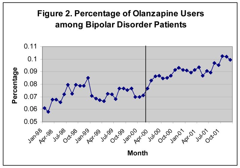
Proportion of Olanzapine Users among Patients with Bipolar Disorder Increases over Time

Figure A-2.

Proportion of Lithium Users among Patients with Bipolar Disorder Decreases over Time

Figure A-3.

Time Trend of Non-Drug Average Spending on Mental Health and Bipolar Disorder Related Services

Table A-1.

Bipolar Disorder Population diagnostic Categories/Hierarchy

Bipolar Disorder I diagnoses:
296.0 Manic disorder, single episode
296.1 Manic disorder, recurrent episode
296.4 Bipolar affective disorder, manic
296.5 Bipolar affective disorder, depressed
296.6 Bipolar affective disorder, mixed
296.7 Bipolar affective disorder, unspecified
Bipolar Disorder II diagnoses:
296.89 Bipolar II disorder
301.11 Chronic hypomanic personality disorder
Bipolar Disorder other diagnoses:
296.80 Manic-depressive psychosis, unspecified
296.81 Atypical manic disorder
296.82 Atypical depressive disorder
301.13 Cychothymic disorder

Notes on how to apply the hierarchy: if number of bipolar disorder I diagnoses is greater than or equal to 1, then study diagnosis is defined as BPAD I; if no bipolar disorder I diagnoses, and the number of bipolar disorder II diagnoses is greater than or equal to one, then study diagnosis is BPAD II; if no bipolar I or II diagnoses, then study diagnosis is BPAD_other.

Table A-2.

Descriptive Statistical Summary of the Unmatched Sample by User Group (219 Olanzapine users and 689 Lithium users)

CHARACTERISTICS	OLANZAPINE	LITHIUM	P–Value
FEMALE	57.412	56.623	0.796
NORTHEAST	28.235	24.017	0.117
NORTHCEN	24.471	22.707	0.500
WEST	1.647	3.348	0.089
SOUTH	39.529	47.016	0.015
FFS	35.765	39.156	0.257
HMO	4.235	7.569	0.026
POSNOCAP	11.294	7.132	0.017
POSCAP	31.765	34.207	0.401
PPO	16.941	11.936	0.019
AGE	43 (15)	40 (15)	0.0001
COUNTMDC1	6 (3)	5 (3)	< 0.0001
ABUSE1	0 (2)	0 (2)	0.810
EPILEP1	0 (1)	0 (0)	0.246
HEART1	1 (3)	0 (4)	0.586
DIABETES1	1 (5)	1 (4)	0.146
THERAPY1	6 (10)	4 (9)	0.0004
NUMBD1	11 (15)	10 (12)	0.259
NUMMH1	19 (20)	15 (16)	0.0050
NUMBDIP1	0 (1)	0 (1)	0.027
NUMBDOP1	11 (15)	10 (12)	0.294
NUMMHIP1	0 (1)	0 (1)	0.0008
NUMMHOP1	18 (20)	15 (16)	0.0064
SUMBD1	2,541 (5,843)	1,960 (4,702)	0.084
SUMBDIP1	1,511 (5,062)	1,158 (3,939)	0.220
SUMBDOP1	1,029 (2,277)	802 (1,688)	0.076
SUMMH1	3,835 (6,971)	2,616 (5,422)	0.0022
SUMMHIP1	2,046 (5,662)	1,410 (4,358)	0.048
SUMMHOP1	1,789 (3,029)	1,206 (2,008)	0.0005
SUMCL1	9,521 (15,194)	5,385 (8,869)	< 0.0001

Notes:

1. Postfix “1” stands for one-year before drug treatment and “2” stands for one-year after drug treatment. Suffix “sum” denotes non-drug spending and “num” denotes the number of claims. “bd” stands for bipolar disorder, “mh” stands for mental health, and “cl” stands for any medical services. “ip” is inpatient care and “op” is outpatient care. For example, sumbdip2 stands for total non-drug spending in bipolar disorder related inpatient services during the year after drug treatment.

2. First few rows in the table are demographic variables, sex, enrollment region, health insurance type and age.

3. Next are some indicators for medical conditions, “countmdc1” measures the number of major diagnostic codes. “Heart1” indicates number of incidents related to heart disease the patient ever had before starting drug treatment, likewise, for epilepsy (EPILEP1), substance abuse (ABUSE1), and diabetes (DIABETES1). “Therapy1” stands for the number of psychology therapies before a patient initiates drug treatment.

4. High s.d. demonstrates high volatility in mental health spending. s.d. measures the variability of data around the mean, which is square root of sample variance, and s.e. measures how well this sample mean estimates population mean.

5. Same notes apply for table 3 in the appendix

Table A-3.

Descriptive Statistical Summary in the Unmatched Sample by Instrument Variable – Before or After March 2000 When Olanzapine was Approved by FDA to Treat Bipolar Disorder (219 olanzapine users and 689 lithium users)

CHARACTERISTICS	After March 00	Before March 00	P–Value
FEMALE	57.500	56.044	0.682
NORTHEAST	32.143	27.002	0.112
NORTHCEN	30.000	22.763	0.020
WEST	2.500	2.983	0.685
SOUTH	30.000	42.700	0.0003
FFS	31.071	40.031	0.010
HMO	12.143	7.064	0.012
POSNOCAP	12.857	7.692	0.013
POSCAP	26.429	29.670	0.317
PPO	17.500	15.542	0.458
USERID	36.429	18.367	< 0.0001
AGE	38 (16)	42 (14)	0.0014
COUNTMDC1	5 (3)	6 (3)	0.321
ABUSE1	1 (3)	0 (3)	0.149
EPILEP1	0 (0)	0 (0)	0.731
HEART1	0 (2)	0 (2)	0.248
DIAB1	1 (4)	1 (4)	0.998
THERAPY1	6 (10)	4 (10)	0.027
NUMBD1	10 (15)	11 (14)	0.063
NUMMH1	17 (21)	16 (17)	0.285
NUMBDIP1	0 (1)	0 (1)	0.023
NUMBDOP1	9 (15)	11 (13)	0.045
NUMMHIP1	0 (1)	0 (1)	0.0015
NUMMHOP1	17 (21)	16 (16)	0.338
SUMBD1	2,093 (4,854)	1,852 (4,179)	0.470
SUMBDIP1	1,392 (4,053)	912 (3,499)	0.086
SUMBDOP1	701 (1,603)	940 (1,820)	0.047
SUMMH1	3,182 (5,775)	2,456 (5,063)	0.070
SUMMHIP1	1,885 (4,588)	1,126 (3,834)	0.016
SUMMHOP1	1,297 (2,063)	1,330 (2,418)	0.830
SUMCL1	6,140 (8,461)	5,308 (8,708)	0.175

References

- Bowden CL. Atypical antipsychotic augmentation of mood stabilizer therapy in bipolar disorder. J Clin Psychiatry. 2005;66(Suppl 3):12–9. [PubMed] [Google Scholar]
- Bowden CL, Lecrubier Y, et al. Maintenance therapies for classic and other forms of bipolar disorder. J Affect Disord. 2000;59(Suppl 1):S57–S67. doi: 10.1016/s0165-0327(00)00179-8. [DOI] [PubMed] [Google Scholar]
- Bridle C, Palmer S, et al. A rapid and systematic review and economic evaluation of the clinical and cost-effectiveness of newer drugs for treatment of mania associated with bipolar affective disorder. Health Technol Assess. 2004;8(19):iii–iv. doi: 10.3310/hta8190. 1-187. [DOI] [PubMed] [Google Scholar]
- Duan N. Stochastic microenvironment models for air pollution exposure. J Expo Anal Environ Epidemiol. 1991;1(2):235–57. [PubMed] [Google Scholar]
- Duggan M. Do new prescription drugs pay for themselves? The case of second-generation antipsychotics. J Health Econ. 2005;24(1):1–31. doi: 10.1016/j.jhealeco.2004.08.001. [DOI] [PubMed] [Google Scholar]
- Kaiser_Family_Foundation “Prescription Drug Trends 2005” http://www.kff.org/insurance/upload/3057-04.pdf.
- Lichtenberg FR. Do (more and better) drugs keep people out of hospitals? Am Econ Rev. 1996;86(2):384–8. [PubMed] [Google Scholar]
- Lichtenberg FR. Are the benefits of newer drugs worth their cost? Evidence from the 1996 MEPS. Health Aff (Millwood) 2001;20(5):241–51. doi: 10.1377/hlthaff.20.5.241. [DOI] [PubMed] [Google Scholar]
- Manning WG. The logged dependent variable, heteroscedasticity, and the retransformation problem. J Health Econ. 1998;17(3):283–95. doi: 10.1016/s0167-6296(98)00025-3. [DOI] [PubMed] [Google Scholar]
- Manning WG, Basu A, et al. Generalized modeling approaches to risk adjustment of skewed outcomes data. J Health Econ. 2005;24(3):465–88. doi: 10.1016/j.jhealeco.2004.09.011. [DOI] [PubMed] [Google Scholar]
- Manning WG, Mullahy J. Estimating log models: to transform or not to transform? J Health Econ. 2001;20(4):461–94. doi: 10.1016/s0167-6296(01)00086-8. [DOI] [PubMed] [Google Scholar]
- Miller GE, Moeller JF, et al. New Cardiovascular Drugs: Patterns of Use and Association with Non-drug Health Expenditures. Inquiry. 2006;42(Winter2005/2006) doi: 10.5034/inquiryjrnl_42.4.397. [DOI] [PubMed] [Google Scholar]
- Muzina DJ, Calabrese JR. Maintenance therapies in bipolar disorder: focus on randomized controlled trials. Australian and New Zealand Journal of Psychiatry. 2005;39(8):652–661. doi: 10.1080/j.1440-1614.2005.01649.x. [DOI] [PubMed] [Google Scholar]
- Namjoshi MA, Risser R, et al. Quality of life assessment in patients with bipolar disorder treated with olanzapine added to lithium or valproic acid. J Affect Disord. 2004;81(3):223–9. doi: 10.1016/j.jad.2003.07.005. [DOI] [PubMed] [Google Scholar]
- Parsons LS. Ovation Research Group; Seattle, WA: 2002. Reducing Bias in a Propensity Score Matched-Pair Sample Using Greedy Matching Techniques. [Google Scholar]
- Tohen M, Chengappa KN, et al. Relapse prevention in bipolar I disorder: 18-month comparison of olanzapine plus mood stabiliser v. mood stabiliser alone. Br J Psychiatry. 2004;184:337–45. doi: 10.1192/bjp.184.4.337. [DOI] [PubMed] [Google Scholar]
- Tohen M, Chengappa KN, et al. Efficacy of olanzapine in combination with valproate or lithium in the treatment of mania in patients partially nonresponsive to valproate or lithium monotherapy. Arch Gen Psychiatry. 2002;59(1):62–9. doi: 10.1001/archpsyc.59.1.62. [DOI] [PubMed] [Google Scholar]
- Tohen M, Greil W, et al. Olanzapine versus lithium in the maintenance treatment of bipolar disorder: a 12-month, randomized, double-blind, controlled clinical trial. Am J Psychiatry. 2005;162(7):1281–90. doi: 10.1176/appi.ajp.162.7.1281. [DOI] [PubMed] [Google Scholar]
- Vieta E, Calabrese JR, et al. Comparison of rapid-cycling and non-rapid-cycling bipolar I manic patients during treatment with olanzapine: analysis of pooled data. J Clin Psychiatry. 2004;65(10):1420–8. doi: 10.4088/jcp.v65n1019. [DOI] [PubMed] [Google Scholar]
- Vieta E, Goikolea JM. Atypical antipsychotics: newer options for mania and maintenance therapy. Bipolar Disorders. 2005;7:21–33. doi: 10.1111/j.1399-5618.2005.00212.x. [DOI] [PubMed] [Google Scholar]
- Vieta E, Reinares M, et al. Olanzapine as long-term adjunctive therapy in treatment-resistant bipolar disorder. J Clin Psychopharmacol. 2001;21(5):469–73. doi: 10.1097/00004714-200110000-00002. [DOI] [PubMed] [Google Scholar]
- Wagner AK, Soumerai SB, et al. Segmented regression analysis of interrupted time series studies in medication use research. J Clin Pharm Ther. 2002;27(4):299–309. doi: 10.1046/j.1365-2710.2002.00430.x. [DOI] [PubMed] [Google Scholar]