Non-steady-state heat conduction in composite walls

Abstract

The problem of heat conduction in one-dimensional piecewise homogeneous composite materials is examined by providing an explicit solution of the one-dimensional heat equation in each domain. The location of the interfaces is known, but neither temperature nor heat flux is prescribed there. Instead, the physical assumptions of their continuity at the interfaces are the only conditions imposed. The problem of two semi-infinite domains and that of two finite-sized domains are examined in detail. We indicate also how to extend the solution method to the setting of one finite-sized domain surrounded on both sides by semi-infinite domains, and on that of three finite-sized domains.

1. Introduction

The problem of heat conduction in a composite wall is a classical problem in design and construction. It is usual to restrict to the case of walls whose constitutive parts are in perfect thermal contact and have physical properties that are constant throughout the material and that are considered to be of infinite extent in the directions parallel to the wall. Further, we assume that temperature and heat flux do not vary in these directions. In that case, the mathematical model for heat conduction in each wall layer is given by [1, ch. 10]

1.1a

and

1.1b

where u^(j)(x,t) denotes the temperature in the wall layer indexed by (j), κ_j>0 is the heat-conduction coefficient of the jth layer (the inverse of its thermal diffusivity), x=a_j is the left extent of the layer and x=b_j is its right extent. The sub-indices denote derivatives with respect to the one-dimensional spatial variable x and the temporal variable t. The function is the prescribed initial condition of the system. The continuity of the temperature u^(j) and of its associated heat flux are imposed across the interface between layers. In what follows, it is convenient to use the quantity σ_j, defined as the positive square root of κ_j: .

If the layer is either at the far left or far right of the wall, Dirichlet, Neumann, or Robin boundary conditions can be imposed on its far left or right boundary, respectively, corresponding to prescribing ‘outside’ temperature, heat flux or a combination of these. A derivation of the interface boundary conditions is found in [1, ch. 1]. It should be noted that the set-up presented in (1.1a) also applies to the case of one-dimensional rods in thermal contact.

In this paper, we use the Fokas method [2–4] to provide explicit solution formulae for different heat transport interface problems of the type described above. We investigate problems in both finite and infinite domains, and we compare our method with classical solution approaches that can be found in the literature. Throughout, our emphasis is on non-steady-state solutions. Even for the simplest of the problems we consider (§3, two finite walls in thermal contact), the classical approach using separation of variables [1] can provide an explicit answer only implicitly. Indeed, the solution obtained in [1] depends on certain eigenvalues defined through a transcendental equation that can be solved only numerically. By contrast, the Fokas method produces an explicit solution formula involving only known quantities. For other problems we consider, to our knowledge no solution has been derived using classical methods and we believe the solution formulae presented here are new.

The representation formulae for the solution can be evaluated numerically, hence the problem can be solved in practice using hybrid analytical–numerical approaches [5] or asymptotic approximations for them may be obtained using standard techniques [3]. The result of such a numerical calculation is shown at the end of §2.

The problem of heat conduction through composite walls is discussed in many excellent texts (see for instance [1,6]). References to the treatment of specific problems are given in the sections below where these problems are investigated. In §2, we investigate the problem of two semi-infinite walls. Section 3 discusses the interface problem with two finite walls. Following that, we consider first the problem of one finite wall between two semi-infinite ones and the problem of three finite walls. Both of them are briefly sketched in §4 and full solutions are presented in the electronic supplementary material.

2. Two semi-infinite domains

In this section, we consider the problem of heat flow through two walls of semi-infinite width or of two semi-infinite rods.

We seek two functions:

satisfying the equations

2.1a

and

2.1b

with the initial conditions being

2.2a

and

2.2b

the asymptotic conditions being

2.3a

and

2.3b

and the continuity interface conditions being

2.4a

and

2.4b

The sub- and super-indices L and R denote the left and right rods, respectively. A special case of this problem is discussed in [1, ch. 10], but only for a specific initial condition. Further, for the problem treated there, both and , are assumed to be zero. This assumption is made for mathematical convenience and no physical reason exists to impose it. If constant (in time) limit values are assumed, a simple translation allows one of the limit values to be equated to zero, but not both. As no great advantage is obtained by assuming a zero limit using our approach, we make the more general assumption (2.3).

We define v^L(x,t)=u^L(x,t)−γ^L and v^R(x,t)=u^R(x,t)−γ^R. Then, v^L(x,t) and v^R(x,t) satisfy

2.5a

2.5b

2.5c

2.5d

2.5e

and

2.5f

At this point, we start by following the standard steps in the application of the Fokas method [2–4]. We begin with the so-called ‘local relations’ [2]

2.6a

and

2.6b

These relations are a one-parameter family obtained by rewriting (2.5a,b).

Applying Green’s formula [7] in the strip in the left-half plane (figure 1), we find

2.7

Figure 1.

Domains for the application of Green’s formula for v^L(x,t) and v^R(x,t). (Online version in colour.)

Let . Similarly, let . As |x| can become arbitrarily large, we require in (2.7) in order to guarantee that the first two integrals are well defined. Let . The region D is shown in figure 2.

Figure 2.

The domains D⁺ and D⁻ for the heat equation. (Online version in colour.)

For , we define the following transforms:

Using these definitions, the global relation (2.7) is rewritten as

2.8

As the dispersion relation ω_L(k)=(σ_Lk)² is invariant under k→−k, so are g₀((σ_Lk)²,t) and g₁((σ_Lk)²,t). Thus, we can supplement (2.8) with its evaluation at −k, namely

2.9

This relation is valid on . Using Green’s formula on (figure 1), the global relation for v^R(x,t) is

2.10

valid in .

As above, using the invariance of ω_R(k)=(σ_Rk)², g₀((σ_Rk)²,t) and g₁((σ_Rk)²,t) under k→−k, we supplement (2.10) with

2.11

for .

Inverting the Fourier transforms in (2.8), we have

2.12

for and t>0. The integrand of the second integral in (2.12) is entire and decays as for . Using the analyticity of the integrand and applying Jordan’s lemma [7], we can replace the contour of integration of the second integral by :

2.13

Proceeding similarly on the right, starting from (2.10), we have

2.14

for and t>0. Here, erf(⋅) denotes the error function: . To obtain the second equality above, we integrated the terms that are explicit.

Expressions (2.13) and (2.14) for v^L(x,t) and v^R(x,t) depend on the unknown functions g₀ and g₁, evaluated at different arguments. These functions need to be expressed in terms of known quantities. To obtain a system of two equations for the two unknown functions, we use (2.9) and (2.10) for g₀((σ_Lk)²,t) and g₁((σ_Lk)²,t). This requires the transformation k→−σ_Lk/σ_R in (2.10). The − sign is required to ensure that both equations are valid on , allowing for their simultaneous solution. We find

2.15

and

2.16

valid for . These expressions are substituted into (2.13) and (2.14). This results in expressions for v^L(x,t) and v^R(x,t) that appear to depend on v^L and v^R themselves. We examine the contribution of the terms involving and . Starting with (2.13), we obtain for v^L(x,t) the following expression:

2.17

for , t>0. The first four terms depend only on known functions. To examine the second-to-last term, we note that the integrand is analytic for all and that decays for for . Thus, by Jordan’s lemma, the integral of along a closed, bounded curve in vanishes. In particular, we consider the closed curve , where and (figure 3).

Figure 3.

The contour is shown as a dashed line. An application of Cauchy’s integral theorem [7] using this contour allows the elimination of the contribution of from integral expression (2.17). Similarly, the contour is shown as a solid line and application of Cauchy’s integral theorem using this contour allows the elimination of the contribution of from integral expression (2.19). (Online version in colour.)

As the integral along vanishes for large C, the fourth integral on the right-hand side of (2.17) must vanish as the contour becomes ∂D⁻ as . The uniform decay of for large k is exactly the condition required for the integral to vanish, using Jordan’s lemma. For the final integral in equation (2.17), we use the fact that is analytic and bounded for . Using the same argument as above, the fifth integral in (2.17) vanishes and we have an explicit representation for v^L(x,t) in terms of initial conditions

2.18

To find an explicit expression for v^R(x,t), we need to evaluate g₀ and g₁ at different arguments, also ensuring that the expressions are valid for . From (2.15) and (2.16), we find

and

Substituting these into equation (2.14), we obtain

2.19

for , t>0. As before, everything about the first three integrals is known. To compute the fourth integral, we proceed as we did before for v^L(x,t) and eliminate integrals that decay in the regions over which we are integrating. The final solution is

2.20

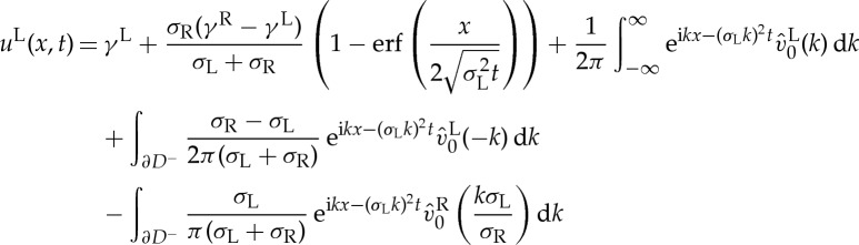
Returning to the original variables, we have the following proposition which determines u^R and u^L fully explicitly in terms of the given initial conditions and the prescribed boundary conditions as .

Proposition 2.1 —

The solution of the heat transfer problem (2.1)–(2.4) is given by

2.21a

and

2.21b

Remarks.

• — The use of the discrete symmetries of the dispersion relation is an important aspect of the Fokas method [2–4]. When solving the heat equation in a single medium, the only discrete symmetry required is k→−k, which was used here as well to obtain (2.9) and (2.11). Owing to the two media, there are two dispersion relations in this problem: ω₁=(σ_Lk)² and ω₂=(σ_Rk)². The collection of both dispersion relations {ω₁,ω₂} retains the discrete symmetry k→−k but admits two additional ones, namely: k→(σ_R/σ_L)k and k→(σ_L/σ_R)k, which transform the two dispersion relations to each other. All non-trivial discrete symmetries of {ω₁,ω₂} are needed to derive the final solution representation, and indeed they are used, for example, to obtain relations (2.15) and (2.16).

• — With σ_L=σ_R and γ^L=γ^R=0, solution formulae (2.21) in their proper x-domain of definition reduce to the solution of the whole line problem as given in [3].

• — Classical approaches to the problem presented in this section can be found in the literature, for the case γ_L=0=γ_R. For instance, for one special pair of initial conditions, a solution is presented in [1]. No explicit solution formulae using classical methods with general initial conditions exist to our knowledge. At best, one is left with having to find the solution of an equation involving inverse Laplace transforms, where the unknowns are embedded within these inverse transforms.

• — The steady-state solution to (2.1) with initial conditions, which decay sufficiently fast to the boundary values (2.3) at , is easily obtained by letting in (2.21). This gives . This is the weighted average of the boundary conditions at infinity with weights given by σ_L and σ_R. To our knowledge, this is a new result. It is consistent with the steady-state limit (γ^L+γ^R)/2 for the whole-line problem with initial conditions that limit to different values γ^L and γ^R as . This result is easily obtained from the solution of the heat equation defined on the whole line using the Fokas method, but it can also be observed by employing piecewise-constant initial data in the classical Green’s function solution, as described in Theorem 4-1 on p. 171 (and comments thereafter) of [8]. It should be emphasized that the steady-state problem for (2.1)–(2.4) or even for the heat equation defined on the whole line with different boundary conditions at and is ill posed in the sense that the steady solution cannot satisfy the boundary conditions.

Using a slight variation on the method presented in [5], one can compute solutions (2.21) numerically with specified initial conditions. We plot solutions for the case of vanishing boundary conditions (γ^L=γ^R=0) with

and

with α_L=25 and α_R=30 (figure 4). The Fourier transforms of these initial conditions may be computed explicitly. We choose σ_L=0.02 and σ_R=0.06. The initial conditions are chosen so as to satisfy interface boundary conditions (2.4) at t=0. The results clearly illustrate the discontinuity in the first derivative of the temperature at the interface x=0.

Figure 4.

Results for solutions (2.18) and (2.20) with , u^R₀(x)= x² e^−(30)2x and σ_L=0.02, σ_R=0.06, γ^L=γ^R=0, t∈[0,0.02] using the hybrid analytical–numerical method of [5]. (Online version in colour.)

3. Two finite domains

Next, we consider the problem of heat conduction through two walls of finite width (or of two finite rods) with Robin boundary conditions. We seek two functions:

satisfying the equations

3.1a

and

3.1b

the initial conditions

3.2a

and

3.2b

the boundary conditions

3.3a

and

3.3b

and the continuity conditions

3.4a

and

3.4b

as illustrated in figure 5, where a>0, b>0 and α_i, 1≤i≤4 constant.

Figure 5.

The heat equation for two finite rods.

If α₁=α₃=0, then Neumann boundary conditions are prescribed, whereas if α₂=α₄=0 then Dirichlet conditions are given.

As before, we have the local relations

3.5a

and

3.5b

We define the time transforms of the initial and boundary data and the spatial transforms of u for as follows:

Using Green’s theorem on the domains [−a,0]×[0,t] and [0,b]×[0,t], respectively, we have the global relations

3.6a

and

3.6b

Both equations are valid for all , in contrast to (2.8) and (2.10). Using the invariance of ω_L(k)=(σ_Lk)² and ω_R(k)=(σ_Rk)² under k→−k, we obtain

3.7a

and

3.7b

Inverting the Fourier transform in (3.6a),

3.8

The integrand of the first integral is entire and decays as for . The second integral has an integrand that is entire and decays as for . It is convenient to deform both contours away from k=0 to avoid singularities in the integrands that become apparent in what follows. Initially, these singularities are removable, as the integrands are entire. Writing integrals of sums as sums of integrals, the singularities may cease to be removable. With the deformations away from k=0, the apparent singularities are no cause for concern. In other words, we deform D⁺ to D⁺₀ and D⁻ to D⁻₀ as shown in figure 6. Thus,

3.9

Figure 6.

Deformation of the contours in figure 2 away from k=0. (Online version in colour.)

To obtain the solution on the right, we apply the inverse Fourier transform to (3.6b)

3.10

The integrand of the first integral is entire and decays as for . The second integral has an integrand that is entire and decays as for . We deform the contours as above to obtain

3.11

Taking the time transform of the boundary conditions results in and

These two equations together with (3.7a,b) are four equations to be solved for the four unknowns , , and . The resulting expressions are substituted in (3.9) and (3.11).

Although we could solve this problem in its full generality, we restrict to the case of Dirichlet boundary conditions (α₂=α₄=0), to simplify the already cumbersome formulae below. Then, and are determined and we solve two equations for two unknowns. System (3.7a,b) is not solvable for and if Δ_L(k)=0, where

It is easily seen that all values of k satisfying this (including k=0) are on the real line. Thus on the contours, the equations are solved without problem, resulting in the expressions below. As before, the right-hand sides of these expressions involve and , evaluated at a variety of arguments. All terms with such dependence are written out explicitly below. Terms that depend on only known quantities are contained in K^L and K^R, the expressions for which are given later.

3.12

and

3.13

where Δ_R(k)=Δ_L(kσ_R/σ_L). The integrands written explicitly in (3.12) and (3.13) decay in the regions around whose boundaries they are integrated. Thus, using Jordan’s lemma and Cauchy’s theorem, these integrals are shown to vanish. Thus, the final solution is given by K^L and K^R.

Proposition 3.1 —

The solution of heat transfer problem (3.1)–(3.4) is given by

3.14

for −a<x<0, and for 0<x<b

3.15

Remarks.

• — The solution of the problem posed in (3.1)–(3.4) may be obtained using the classical method of separation of variables and superposition [1]. The solutions u^L(x,t) and u^R(x,t) are given by a series of eigenfunctions with eigenvalues that satisfy a transcendental equation, closely related to the equation Δ_L(k)=0. This series solution may be obtained from proposition 3.1 by deforming the contours along and to the real line, including small semicircles around each root of either Δ_L(k) or Δ_R(k), depending on whether u^L(x,t) or u^R(x,t) is being calculated. Indeed, this is allowed because all integrands decay in the wedges between these contours and the real line, and the zeros of Δ_L(k) and Δ_R(k) occur only on the real line, as stated above. Careful calculation of all different contributions, following the examples in [2,3], shows that the contributions along the real line cancel, leaving only residue contributions from the small circles. Each residue contribution corresponds to a term in the classical series solution. It is not necessarily beneficial to leave the form of the solution in proposition 3.1 for the series representation, as the latter depends on the roots of Δ_L(k) and Δ_R(k), which are not known explicitly. By contrast, the representation of proposition 3.1 depends on known quantities only and may be readily computed, using one’s favourite parameterization of the contours and .

• — Similarly, the familiar piecewise linear steady-state solution of (3.1)–(3.4) with Dirichlet boundary conditions [1] can be observed from (3.14) and (3.15) by choosing initial conditions that decay appropriately and constant boundary conditions f_L(t)=γ^L and f_R(t)=γ^R. It is convenient to choose zero initial conditions, as the initial conditions do not affect the steady state. As above, the contours are deformed so that they are along the real line with semicircular paths around the zeros of Δ_L(k) and Δ_R(k), including k=0. As one of these deformations arises from while the other comes from , the contributions along the real line cancel each other, while the semicircles add to give full residue contributions from the poles associated with the zeros of Δ_L(k). All such residues vanish as , except at k=0. It follows that the steady-state behaviour is determined by the residue at the origin. This results in

  

  and

  

  which is piecewise linear and continuous.
• — A more direct way to recover only the steady-state solution to (3.1) with and constant is to write the solution as the superposition of two parts: and . The first parts and satisfy the boundary conditions as and the stationary heat equation. In other words,

  

  A piecewise linear ansatz with the imposition of the interface conditions results in linear algebra for the unknown coefficients [1]. With the steady-state solution in hand, the second (time-dependent) parts and satisfy the initial conditions modified by the steady-state solution and the boundary conditions minus their value as

  

  where, as usual, we impose continuity of temperature and heat flux at the interface x=0. The dynamics of the solution is described by and , both of which decay to zero as . Their explicit form is easily found using the method described in this section.

4. Other problems

With the basic principles of the method outlined in the previous two sections, problems with more layers, both finite and infinite, may be addressed. We state two additional problems below and include solutions for specific initial conditions. More complete solutions can be found in the electronic supplementary material.

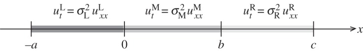
(a). Infinite domain with three layers

In this section, we consider the heat equation defined on two semi-infinite rods enclosing a single rod of length 2a.

We seek three functions:

with t≥0, satisfying the equations

4.1a

4.1b

and

4.1c

with the initial conditions being

4.2a

4.2b

and

4.2c

the asymptotic conditions being

4.3a

and

4.3b

and the continuity conditions being

4.4a

4.4b

4.4c

and

4.4d

as shown in figure 7.

Figure 7.

The heat conduction problem for a single rod of length 2a between two semi-infinite rods.

Asymptotic conditions (4.3) are not the most general possible but are used here to simplify calculations. To our knowledge, no aspect of this problem is addressed in the literature.

To solve this problem, one would proceed with the following steps:

• (i) Write the local relations in each of the three domains: left, middle and right.

• (ii) Use Green’s theorem to define the three global relations, keeping track of where they are valid in the complex k plane.

• (iii) Solve the three global relations for u^L(x,t), u^M(x,t) and u^R(x,t) by inverting the Fourier transforms.

• (iv) Using the k→−k symmetry of the dispersion relationships on the three original global relations, write down three more global relations. This uses the discrete symmetry of each individual dispersion relation.

• (v) Deform the integrals of the solution expressions to or as dictated by the region of analyticity of the integrand.

• (vi) Use the discrete symmetries of the dispersion relationship to the collection of global relations for g₀(ω,t), g₁(ω,t), h₀(ω,t) and h₁(ω,t). Care should be taken that relations can only be solved simultaneously provided their regions of validity overlap. At this stage, as in the previous two sections, the discrete symmetries from one dispersion relation to another come into play.

• (vii) Terms containing unknown functions are shown to be zero by examining the regions of analyticity and decay for the relevant integrands and the use of Jordan’s lemma.

For brevity of the presentation, we will assume that u^M(x,0)=0=u^R(x,0). The solution to the non-restricted problem can be found in the electronic supplementary material. After defining the transforms

we proceed as outlined above. The solution formulae are given in the following proposition:

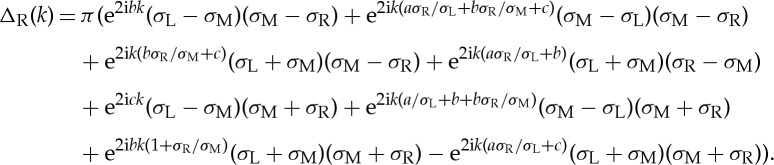
Proposition 4.1 —

The solution of the heat transfer problem (4.1)–(4.4) with u^M(x,0)=u^R(x,0)=0 is

for with Δ_L(k)=π((σ_L−σ_M)(σ_M−σ_R)+e^{4iakσ_L/σ_M}(σ_L+σ_M)(σ_M+σ_R)),

for −a<x<b with Δ_R(k)=π((σ_L+σ_M)(σ_M+σ_R)+e^{4iakσ_R/σ_M}(σ_L−σ_M)(σ_M−σ_R)). Lastly, the expression for u^R(x,t), valid for x>a, is

(b). Finite domain with three layers

We consider the heat conduction problem in three rods of finite length as shown in figure 8.

Figure 8.

The heat equation for three finite layers.

We seek three functions:

satisfying the equations

4.5a

4.5b

and

4.5c

with the initial conditions being

4.6a

4.6b

and

4.6c

the boundary conditions being

4.7a

and

4.7b

and the continuity conditions being

4.8a

4.8b

4.8c

and

4.8d

The solution process is as before, following the steps outlined in the previous section. For simplicity, we assume Neumann boundary data (α₁=α₃=0), zero boundary conditions (f^L(t)=f^R(t)=0) and u^M(x,0)=0=u^R(x,0). The solution with u^M(x,0)≠0 and u^R(x,0)≠0 is given in the electronic supplementary material. We define

The solution is given by the following proposition:

Proposition 4.2 —

The solution to the heat transfer problem (4.5)–(4.8) with α₁=α₃=0, f^L(t)=f^R(t)=0 and u^M(x,0)=u^R(x,0)=0 is

for −a<x<0 with

Next,

for 0<x<b, with

and

for b<x<c with

Funding statement

This work was generously supported by the National Science Foundation under grant no. NSF-DMS-1008001 (B.D., N.E.S.). N.E.S. also acknowledges support from the National Science Foundation under grant no. NSF-DGE-0718124.

References

- 1.Hahn D, Özisik M. 2012. Heat conduction Hoboken, NJ: John Wiley & Sons, Inc; 3rd edn. [Google Scholar]
- 2.Deconinck B, Trogdon T, Vasan V. 2014. The method of Fokas for solving linear partial differential equations. SIAM Rev. 56, 159–186 (doi:10.1137/110821871) [Google Scholar]
- 3.Fokas AS. 2008. A unified approach to boundary value problems. CBMS-NSF Regional Conference Series in Applied Mathematics, vol. 78 Philadelphia, PA: Society for Industrial and Applied Mathematics (SIAM) [Google Scholar]
- 4.Fokas AS, Pelloni B. 2005. A transform method for linear evolution PDEs on a finite interval. IMA J. Appl. Math. 70, 564–587 (doi:10.1093/imamat/hxh047) [Google Scholar]
- 5.Flyer N, Fokas AS. 2008. A hybrid analytical-numerical method for solving evolution partial differential equations. I. The half-line. Proc. R. Soc. A 464, 1823–1849 (doi:10.1098/rspa.2008.0041) [Google Scholar]
- 6.Carslaw HS, Jaeger JC. 1959. Conduction of heat in solids, 2nd edn. New York, NY: Oxford University Press [Google Scholar]
- 7.Ablowitz MJ, Fokas AS. 2003. Complex variables: introduction and applications, 2nd edn, Cambridge Texts in Applied Mathematics Cambridge, UK: Cambridge University Press [Google Scholar]
- 8.Guenther RB, Lee JW. 1996. Partial differential equations of mathematical physics and integral equations. Mineola, NY: Dover Publications Inc. (Corrected reprint of the 1988 original.) [Google Scholar]