Cognitive control over learning: Creating, clustering and generalizing task-set structure

Abstract

Executive functions and learning share common neural substrates essential for their expression, notably in prefrontal cortex and basal ganglia. Understanding how they interact requires studying how cognitive control facilitates learning, but also how learning provides the (potentially hidden) structure, such as abstract rules or task-sets, needed for cognitive control. We investigate this question from three complementary angles. First, we develop a new computational “C-TS” (context-task-set) model inspired by non-parametric Bayesian methods, specifying how the learner might infer hidden structure and decide whether to re-use that structure in new situations, or to create new structure. Second, we develop a neurobiologically explicit model to assess potential mechanisms of such interactive structured learning in multiple circuits linking frontal cortex and basal ganglia. We systematically explore the link betweens these levels of modeling across multiple task demands. We find that the network provides an approximate implementation of high level C-TS computations, where manipulations of specific neural mechanisms are well captured by variations in distinct C-TS parameters. Third, this synergism across models yields strong predictions about the nature of human optimal and suboptimal choices and response times during learning. In particular, the models suggest that participants spontaneously build task-set structure into a learning problem when not cued to do so, which predicts positive and negative transfer in subsequent generalization tests. We provide evidence for these predictions in two experiments and show that the C-TS model provides a good quantitative fit to human sequences of choices in this task. These findings implicate a strong tendency to interactively engage cognitive control and learning, resulting in structured abstract representations that afford generalization opportunities, and thus potentially long-term rather than short-term optimality.

1 Introduction

Life is full of situations that require us to appropriately select simple actions, like clicking Reply rather than Delete to an email, or more complex actions requiring cognitive control, like changing modes of operation when switching from a Mac to a Linux machine. These more complex actions themselves define simple rules, or task-sets, i.e., abstract constructs that signify appropriate stimulus-response groupings in a given context (Monsell, 2003). Extensive task-switching literature has revealed the existence of task-set representations in both mind and brain (fMRI: Dosenbach et al. (2006), monkey electrophysiology: Sakai (2008), etc). Notably, these task-set representations are independent of the context in which they are valid (Reverberi et al., 2011; Woolgar et al., 2011) and even of the specific stimuli and actions to which they apply (Haynes et al., 2007), and are thus abstract latent constructs that constrain simpler choices.

Very little research addresses how such task-sets are constructed during uninstructed learning, and for what purpose (i.e. do they facilitate learning?). Task-switching studies are typically supervised: the relevant rule is explicitly indicated and the rules themselves are either well known (e.g., arrows pointing to the direction to press) or highly trained (e.g., vowel-consonant discriminations). In some studies, participants need to discover when a given rule has become invalid and switch to a new valid rule from a set of known candidate options (Nagano-Saito et al., 2008; Mansouri et al., 2009; Imamizu et al., 2004; Yu & Dayan, 2005; Hampton et al., 2006), without having to learn the nature of the rules themselves. Conversely, the reinforcement learning literature has largely focused on how a single rule is learned and potentially adapted, in the form of a mapping between a set of stimuli and responses.

However, we often need to solve these two problems simultaneously: in an unknown context, the appropriate rules might be completely new and hence need to be learned, or they might be known rules that only need to be identified as valid, and simply reused in the current context. How do humans simultaneously learn (i) the simple stimulus-response associations that apply for a given task-set, and (ii) at the more abstract level, which of the candidate higher order task-set rules to select in a given context (or whether to build a new one)? Though few studies have confronted this problem directly, a few of them have examined simultaneous learning at different hierarchical levels of abstraction. For example, subjects learned more efficiently when a simplifying rule-like structure was available in the set of stimulus-action associations to be learned (“policy abstraction”, Badre et al., 2010). Collins & Koechlin (2012) showed that subjects build repertoires of task-sets, and learn to discriminate between whether they should generalize one of the stored rules or learn a new one in a new temporal context. Both studies thus showed that when structure was available in the learning problem (signified by either contextual cues or by temporal structure), subjects were able to discover such structure and make efficient use of it to speed learning. However, these studies do not address whether and how subjects spontaneously and simultaneously learn such rules and sets of rules when the learning problem does not in some way cue that organization. One might expect such structure building in part because it may afford a performance advantage for subsequent situations that permit generalization of learned knowledge.

Here, we develop computational models to explore the implications of building task-set structure into learning problems, whether or not there is an immediate advantage to doing so. We then examine how, when confronted with new contexts, humans and models can decide whether to re-use existing structured representations or to create new ones.

We have thus far considered how rules requiring cognitive control (task-sets) are created and learned. We now turn to the reciprocal question needed to close the loop: how does cognitive control facilitate learning?

For example, the computational reinforcement learning (RL) framework typically assumes that subjects learn for each state (e.g., observed stimulus) to predict their expected (discounted) future rewards for each of the available actions. These state-action reward values are used to determine the appropriate action to select (e.g., Sutton & Barto, 1998; Samejima et al., 2005; Daw & Doya, 2006; Frank et al., 2007a). Most reinforcement learning studies assume that the relevant state space is known and fully observable. However, there could be uncertainty about the nature of the state to be learned, or this state might be hidden (e.g., it may not represent a simple sensory stimulus, but could be, for example, a sequential pattern of stimuli, or it could depend on the subject’s own previous actions). When given explicit cues informative about these states (but not which actions to take), participants are much more likely to discover the optimal policy in such environments (Gureckis & Love, 2010). Without such cues, learning requires making decisions based on the (partially) hidden states. Thus, cognitive control may be necessary for hypothesis testing about current states which act as contexts for learning motor actions (e.g., treating the internally maintained state as if it was an observable stimulus in standard RL).

Indeed, recent behavioral modeling studies have shown that subjects can learn hidden variables such as latent states relevant for action selection, as captured by Bayesian inference algorithms or approximations thereof (Redish et al., 2007; Gershman et al., 2010; Todd et al., 2009; Frank & Badre, 2011; Collins & Koechlin, 2012; Wilson & Niv, 2011). In most of these studies, there is a clear advantage to be gained by learning these hidden variables, either in optimizing learning speed (Behrens et al., 2007), or to separate superficially similar conditions into two different latent states. Thus learning often implicates more complex strategies including identification and manipulation of hidden variables. Some studies have shown that subjects even tend to infer hidden patterns in the data when they do not exist and afford no behavioral advantage (Yu & Cohen, 2009), or when it is detrimental to do so (Gaissmaier & Schooler, 2008; Lewandowsky & Kirsner, 2000). Thus humans may exhibit a bias to use more complex strategies even when they’re not useful, potentially because these strategies are beneficial in many real life situations.

We can thus predict that subjects might adopt this same approach to create task-set structure – identifying cues as indicative of task-sets which contextualize lower level stimulus-response mappings – when learning very simple stimulus-action associations that require no such structure. This prediction relies on the three previously described premises found in the literature:

1. when cued, rules requiring cognitive control can be discovered and leveraged;

2. learning may involve complex cognitive control-like strategies which can in turn improve learning;

3. subjects have a bias to infer more structure than needed in simple sequential decision tasks.

The first two points define the reciprocal utility of cognitive control and learning mechanisms. The third point implies that there must be an inherent motivation for building such structure. One such motivation, explored in more detail below, is that applying structure to learning of task-sets may afford the possibility of reusing these task-sets in other contexts, thus affording generalization of learned behaviors to future new situations. Next, we motivate the development of computational models inspired by prior work in the domain of category learning but extended to handle the creation and re-use of task-sets in policy selection.

1.1 Computational models of reinforcement learning, category learning, and cognitive control

Consider the problem of being faced with a new electronic device (e.g., your friend’s cell phone) or a new software tool. Although these examples constitute new observable contexts or situations, figuring out the proper actions often does not require to relearn from “scratch”. Instead, with just a little trial and error, we can figure out the general class of software or devices to which this applies, and act accordingly. Occasionally, however, we might need to recognize a veridical novel context that requires new learning, without unlearning existing knowledge (e.g., learning actions for a Mac without interfering with actions for a PC). In the problems we define below, people need to learn a set of rules (hidden variables) that is discrete but of unknown size, informed by external observable cues and which serve to condition the observed stimulus-action-feedback contingencies. They also need to infer the current hidden state/rule for action selection in any given trial. Three computational demands are critical for this sort of problem:

1. the ability to represent a rule in an abstract form, dissociated from the context with which it has been typically associated, as is the case for task-sets (Reverberi et al., 2011; Woolgar et al., 2011), such that it is of potentially general rather than local use;

2. the ability to cluster together different arbitrary contexts linked to a similar abstract task-set;

3. the ability to build a new task-set cluster when needed, to support learning of that task-set without interfering with those in other contexts.

This sort of problem can be likened to a class of well-known nonparametric Bayesian generative processes, often used in Bayesian models of cognition, Chinese restaurant processes (Blei et al., 2004)¹. Computational approaches suitable for addressing the problem of inferring hidden rules (and where the number of rules is unknown) include Dirichlet process mixture models (e.g. Teh et al., 2006) and infinite partially observable Markov decision processes (iPOMDP; Doshi, 2009). This theoretical framework has been successfully leveraged in the domain of category learning (e.g. Sanborn et al., 2006, 2010; Gershman et al., 2010; Gershman & Blei, 2012), where latent category clusters are created that allow principled grouping of perceptual inputs to support generalization of learned knowledge, even potentially inferring simultaneously more than one possible relevant structure for categorization (Shafto et al., 2011). Further, although optimal inference is too computationally demanding and has high memory cost, reasonable approximations have been adapted to account for human behavior (Sanborn et al., 2010; Anderson, 1991).

Here, we take some inspiration from these models of perceptual clustering and extend them to support clustering of more abstract task-set states which then serve to contextualize lower level action selection. We discuss the relationship with our work and the category learning models in more detail in the General Discussion. In brief, the perceptual category learning literature typically focuses on learning categories based on similarity between multidimensional visual exemplars. In contrast, useful clustering of contexts for defining task-sets relies not on their perceptual similarity but rather in their linking to similar stimulus-action-outcome contingencies (Figure 1, only one ‘dimension’ of which are observable in any given trial. We thus extend similarity-based category learning from the mostly observable perceptual state-space to an abstract, mostly hidden but partially observable rule space.

Figure 1. Task-set clustering vs perceptual category clustering.

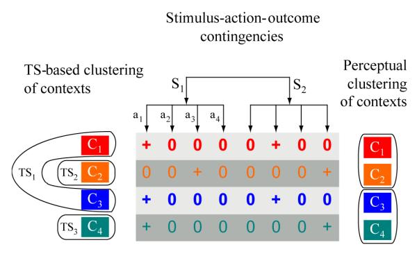
A task-set defines a set of (potentially probabilistic) stimulus-action-outcome (S-A-O) contingencies, depicted here with deterministic binary outcomes for simplicity. To identify similarity between disparate contexts pointing to the same latent task-set (left), the agent has to actively sample and experience multiple distinct S-A-O contingencies across trials (only one S and one A from the potentially much larger set is observable in a single trial). In contrast, in perceptual category learning, clustering is usually built from similarity among perceptual dimensions (shown simplistically here as color grouping, right), with all (or most) relevant dimensions observed at each trial. Furthermore, from the experimenter perspective, subject beliefs about category labels are observed directly by their actions; in contrast, abstract task-sets remain hidden to the experimenter (e.g., the same action can apply to multiple task-sets and a single task-set consists of multiple S-A contingencies).

In a mostly separate literature, computational models of cognitive control and learning have been fruitfully applied to studying a wide range of problems. However, these too have limitations. In the vast majority, learning problems are modeled with RL algorithms that assume perfect knowledge of the state, although some recent models include state uncertainty or learning about problem structure in specific circumstances (Acuña & Schrater, 2010; Kruschke, 2008; Nassar et al., 2010; Green et al., 2010; Wilson & Niv, 2011; Botvinick, 2008; Frank & Badre, 2011; Collins & Koechlin, 2012).

Thus our contribution here is to establish a link between the clustering algorithms of category learning models on the one hand, and the task-set literature and models of cognitive control and reinforcement learning on the other. The merger of these modeling frameworks allows us to address the computational tradeoffs inherent in building vs. reusing task-sets for guiding action selection and learning. We propose a new computational model inspired by the Dirichlet process mixture framework, while including reinforcement learning heuristics simple enough to allow for quantitative trial by trial analysis of subjects’ behavior. This simplicity allows us to assume a plausible neural implementation of this approximate process, grounded by the established and expanding literature on the neurocomputational mechanisms of reinforcement learning and cognitive control. In particular, we show that a multiple loop corticostriatal gating network using reinforcement learning can implement the requisite computations to allow task-sets to be created or re-used. The explicit nature of the mechanisms in this model allows us to derive predictions regarding the effects of biological manipulations, and disorders on structured learning and cognitive control. Because it is a process model it also affords predictions about the dynamics of action selection within a trial, and hence response times.

1.2 Neural mechanisms of learning and cognitive control

Many neural models of learning and cognitive control rely on the known organization of multiple parallel frontal cortico-basal ganglia loops (Alexander & DeLong, 1986). These loops implement a gating mechanism for action selection, facilitating selection of the most rewarding actions while suppressing less rewarding actions, where the reward values are acquired via dopaminergic reinforcement learning signals (e.g. Doya, 2002; Frank, 2005). Moreover, the same mechanisms have been co-opted to support the gating of more cognitive actions, such as working memory updating and maintenance via loops connecting more anterior prefrontal regions and basal ganglia (Frank et al., 2001; O’Reilly & Frank, 2006; Gruber et al., 2006; Todd et al., 2009).

In particular, O’Reilly & Frank (2006) have shown how multiple PFC-BG circuits can learn to identify and gate stimuli into working memory, and to represent these states in active form such that subsequent motor responses can be appropriately contextualized. Todd et al. (2009) provided an analysis of this gating and learning process in terms of POMDPs. Recently, Frank & Badre (2011) proposed a hierarchical extension of this gating architecture for increasing efficiency and reducing conflict when learning multiple tasks. Noting the similarity between learning to choose a higher order rule, and learning to select an action within a rule, they implement these mechanisms in parallel gating loops, with hierarchical influence of one loop over another. This generalized architecture enhanced learning and, when reduced to a more abstract computational level model, provided quantitative fits to human subjects behavior, with support for its posited mechanisms provided by functional imaging analysis (Frank & Badre, 2011; Badre et al., 2012). However, neither that model nor its predecessors can account for the sort of task-set generalization to novel contexts afforded by the iPOMDP framework and observed in the experiments reported below. We thus develop a novel hierarchical extension of the cortico-basal ganglia architecture to simultaneously support the selection of abstract task-sets in response to arbitrary cues, and of actions in response to stimuli, contextualized by the abstract rule.

The remainder of the paper is organized as follows. We first present the C-TS model, an approximate non-parametric Bayesian framework for creation, learning and clustering task-set structure and show that it supports improved performance and generalization when multiple contextual states are indicative of previously acquired task-sets. We consider cases in which building task-set structure is useful for improving learning efficiency and also when it is not. We then show how this functionality can be implemented in a nested corticostriatal neural network model, with associated predictions about dynamics of task-set and motor response selection. We provide a principled linking between the two levels of modeling to show how selective biological manipulations in the neural model are captured by distinct parameters within the non-parametric Bayesian framework. This formal analysis allows us to derive a new behavioral task protocol to assess human subjects’ tendency to incidentally build, use, and transfer task-set structure without incentive to do so. We validate these predictions in two experiments.

2 C-TS Model description

We first present the C-TS model for building TS-structure given a known context and stimulus space. Below we extend this to the general case allowing inference about which input dimension constitutes context, which constitutes lower level stimulus, and whether this hierarchical structure is present at all.

2.1 C-TS Model

We begin by describing the problem in terms of the following structure. As in standard RL problems, at each time t the agent needs to select an action a_t that, depending on the current state (sensory input), leads to reinforcement r_t. We confront the situation in which the link between state and action depends on higher task-set rules which are hidden (and of unknown size, i.e. the learner does not know how many different rules exist). To do so, we assume that the state is itself determined hierarchically. Specifically, we assume that the agent considers some input dimensions to act as higher order context c_t potentially indicative of a task-set, and other dimensions to act as lower level stimulus s_t for determining which motor actions to produce. In the examples we consider below, c_t could be a color background in an experiment, and s_t could be a shape.

We further assume that at any point in time, a non observable variable indicates the valid rule or task-set TS_t and determines the contingencies of reinforcement: P(r_t∣s_t, a_t, c_t) = ∑TS_i P(r_t∣s_t, a_t, TS_i)P(TS_i∣c_t). For simplicity, we assume probabilistic binary feedback, such that P(r_t∣s_t, a_t, TS_t) are Bernoulli probability distributions. In words, the action that should be selected in the current state is conditioned on the latent task set variable TS_t, which is itself cued by the context. Note that there is not necessarily a one-to-one mapping from contexts to task-sets: indeed, a given task-set may be cued by multiple different contexts. We assume that the prior on clustering of the task-sets corresponds to a Dirichlet (“chinese restaurant”) process: if contexts {c_1:n} are clustered on N ≤ n task-sets, then for any new context c_n+1 ∉ {c_1:n},

$$\begin{array}{cc}\hfill P(\mathit{TS}=N+1\mid c_{n+1})& =\alpha ∕A\hfill \\ \hfill P(\mathit{TS}=i\mid c_{n+1})& =N_i∕A\hfill \end{array}$$ (1)

Where N_i is the number of contexts clustered on task-set i, α > 0 is a clustering parameter and A = α + ∑_k=1…N N_k = α + N is a normalizing constant (Gershman et al., 2010). Thus, for each new context, the probability of creating a new task-set is proportional to α, and the probability of reusing one of the known task-sets is proportional to the popularity of that task-set across multiple other contexts.

We do not propose that humans solve the inference problem posed by such a generative model. Indeed, near optimal inference is computationally extremely demanding both in memory and computation capacities, which does not fit with our objective of representing the learning problem as an online, incremental and efficient process in a way that may be plausibly achieved by human subjects. Instead, we propose a reinforcement-learning-like algorithm that approximates this inference process well enough to produce adequate learning and generalization abilities, but simple enough to be plausibly carried out and to allow analysis of trial-by-trial human behavior. Nevertheless, as a benchmark, we did simulate a more exact version of the inference process using a particle filter with large number of particles. As expected, learning overall is more efficient with exact inference, but all qualitative patterns presented below for the approximate version are similar.

The crucial aims of the C-TS model are (i) to create representations of task-set (TS) and of their parameters (stimulus-response-outcome mappings); (ii) to infer at each trial which TS is applicable and should thus guide action selection; and (iii) to discover the unknown space of hidden TS rules. Given that a particular TS_i is created, the model must learn predicted reward outcomes following action selection in response to the current stimulus P(r∣s, a, TS_i). We assume Beta probability distribution priors on the parameter of the Bernoulli distribution. Identification of the valid hidden TS rule is accomplished through Bayesian inference, as follows. For all TS_i in the current TS space, and all contexts c_j, we keep track of the probability that this task-set is valid given the context, p(TS_i∣c_j), and the most probable task-set TS_t in context c_t is used for action selection. Specifically, after observation of reward outcome, the estimated posterior validities of all TS_i are updated:

$$P_{t+1}({\mathit{TS}}_i\mid c_t)=\frac{P(r_t\mid s_t,a_t,{\mathit{TS}}_i)\times P({\mathit{TS}}_i\mid c_t)}{\sum _{j=1\dots N_{\mathit{TS}}\left(t\right)}P(r_t\mid s_t,a_t,{\mathit{TS}}_j)\times P({\mathit{TS}}_j\mid c_t)]},$$ (2)

where N_TS(t) is the number of task-sets created by the model up to time t (see details below), and all probabilities are implicitly conditioned on past history of trials. This ex-post calculation determines the most likely hidden rule corresponding to the trial once the reward has been observed. We assign this trial definitively to that particular latent state, rather than keeping track of the entire probability history. This posterior then determines (i) which task-set’s parameters (stimulus-action associations) is updated, and (ii) the inferred task-set on subsequent encounters of context c_t. Motor action selection is then determined as a function of the expected reward values of each stimulus action pair given the TS, Q(s, a_k) = E(r∣s_t, a_k, TS_t), where the choice function can be greedy or noisy, for example softmax (see equation 4)².

The last critical aspect of this model is the building of the hidden TS space itself, the size of which is unknown. Each time a new context is observed we allow the model the potential to be linked to a TS in the existing set or to expand the considered TS space, such that N_TS(t + 1) = N_TS(t) + 1. Thus, upon each first encounter of a context c_n+1, we increase the current space of possible hidden TS by adding a new (blank) TS_new to that space (formally, a blank TS is defined by initializing P(r∣s, a, TS_new) to an uninformative prior). We then initialize the prior probability that this new context is indicative of TS_new or whether it should instead be linked to an existing TS, as follows.

$$P({\mathit{TS}}^{\ast }=.\mid c_{n+1})=\{\begin{array}{ccc}\hfill P({\mathit{TS}}^{\ast }={\mathit{TS}}_{\mathit{new}}\mid c_{n+1})& \hfill =\hfill & \alpha ∕A\hfill \\ \hfill \forall i\ne \mathit{new},P({\mathit{TS}}^{\ast }={\mathit{TS}}_i\mid c_{n+1})& \hfill =\hfill & \sum _{j}P({\mathit{TS}}_i\mid c_j)∕A\hfill \end{array}\phantom{\}}$$ (3)

Here, α determines the likelihood of visiting a new TS state (as in a Dirichlet / Chinese restaurant process), and A is a normalizing factor: A = α + ∑i,j P(TS_i∣c_j). Intuitively, this prior allows a popular TS to be more probably associated to the new context, weighed against factor α determining the likelihood of constructing a new hidden rule. α can be thought of as a clustering parameter, with lower values yielding more clustering of new contexts to existing TS’s.³ Note that the new task-set might never have been estimated as valid either a priori (and thus never chosen), or a posteriori (and thus remain blank). Therefore, multiple contexts could feasibly link to the same TS and the number of filled (not blank) task-sets does not need to increase proportionally with the number of contexts. We can estimate the expected number of existing TS by summing across all potential TS their expected probability across contexts. Finally, note that since there is no backward inference, and only one history of assignments is tracked (partly analogous to a particle filter with a single particle), we use probabilities rather than discrete number assignments to clusters to initialize the prior. The approximation made in the Bayesian inference, which in its exact form would require keeping track of all possible clustering of previous trials and summing over them, which is computationally intractable, means that at each trial, we collapse the joint posterior on a single high probability task-set assignment. We still keep track of and propagate uncertainty about that assignment and the clustering of contexts, but forget uncertainty about the specific earlier assignments.

2.2 Flat model

As a benchmark, we compare the above structured C-TS model’s behavior to a “flat” learner model, which represents and learns all inputs independently from one-another (ie. so that contexts are treated just like other stimuli; fig 11a). We refer readers to the appendix for details. Briefly, the flat model represents the “state” as the conjunction of stimulus and context and then estimates expected reward for state-action pairs, Q((c_t, s_t), a_t).

Figure 11. Various Model Predictions.

(a,c,e,f) Graphical representation of model information structures. Grey areas represent test-phase only associations. (b,d,g) Model test phase predictions for the transfer condition (blue) and the new condition (green): Proportion of correct responses as a function of input repetition, inset: proportion of errors of type; neglect color (NC), neglect shape (NS) or neglect all (NA). Model simulations were conducted using parameters chosen for best model performance within a qualitatively representative range, over 1000 repetitions. a) Flat model: all input-action associations are represented independently of each other (ie conjunctively). b) The flat model predicts no effect of test condition on learning or error type. c) Dimension-experts model. Appropriate actions for shapes and colors are represented separately. In the test phase the shape expert does not have any new links to learn (no new shapes, no new correct actions for the old shapes in new colors), while the color expert learns links for the new colors. d) No effect of test condition in this model, but a main effect of error type. e) S-TS(c) structure model: shape acts as a context for selecting task-sets that determine color stimulus-action associations, so that new test-phase colors are new stimuli to be learned within already created task-sets. Predictions for this model are qualitatively the same as for the dimension experts model (d). f) C-TS(s) structure model: color context determines a latent task-set, that contextualizes the learning of shape stimulus-action asociations. The C3 transfer context may be linked to TS1, whereas the C4 new context should be assigned to a new task-set. Curbed arrows indicate different kinds of errors: NS, NC or NA. g) C-TS(s) model predicts faster learning for test transfer condition than test new condition, and an interaction between condition and error type.

Policy is determined by the commonly used softmax rule for action selection as a function of the expected reward for each action:

$$p_{\mathit{flat}}\left(a\right)=\mathit{softmax}\left(a\right)=\frac{\mathit{exp}\left(\beta Q\right((c_t,s_t),a\left)\right))}{\sum _{a^{\prime }}\mathit{exp}\left(\beta Q\right((c_t,s_t),a^{\prime }\left)\right))},$$ (4)

where β is an inverse temperature parameter determining the degree of exploration vs exploitation, such that very high β values lead to a greedy policy.

2.3 Generalized structure model

The C-TS model described earlier arbitrarily imposed one of the input dimensions (C) as the context cueing the task-sets, and the other (S) acting as stimulus to be linked to an action according to the defined task-set. We will denote S-TS the symmetrical model that would have made the contrary assignment of input dimensions.

A more adaptive inference model would not choose one fixed dimension as context but instead would infer the identity of the contextual dimension. Indeed, the agent should be able to infer whether there is task-set structure at all. We thus develop a generalized model that simultaneously considers potential C-TS structure, S-TS structure, or flat structure and makes inferences about which of these generative models is valid. For more details, see the appendix.

3 C-TS Model behavior

3.1 Initial clustering

We first simulated the C-TS model to verify that this approximate inference model can leverage structure and appropriately cluster contexts around corresponding abstract task-sets when such structure exists. We therefore first simulated a learning task in which there is a strong immediate advantage to learning structure (see figure 2, top left). This task included sixteen different contexts and three stimuli, presented in interleaved fashion. Six actions were available to the agent. Critically, the structure was designed so that eight contexts were all indicative of the same task-set TS₁, while the other eight signified another task-set TS₂. Feedback was binary and deterministic.

Figure 2. Paradigms used to assess task-set clustering as a function of clustering parameter α.

Top: Initial clustering benefit task: demonstration of advantage to clustering during a learning task in which there are 16 “redundant” contexts, signifying just two distinct TS (see protocol on the left). Speeded learning is observed for structured model (with low Dirichlet parameter α = 1, thus high prior for clustering), compared to flat learning model (high α, so that state-action-outcome mappings are learned separately for each context). Bottom: Structure transfer task: Effect of clustering on subsequent transfer, when there is no advantage to clustering during initial learning (protocol on left). Bottom middle. Proportion of correct responses as a function of clustering α parameter in the first 10 trials, for C3 transfer (blue) and C4 new (green) test conditions. Large α’s indicate a strong prior to assign a new hidden state to a new context, thus leading to no performance difference between conditions. Low α’s indicate a strong prior to re-use existing hidden states in new contexts, leading to positive transfer for C3, but negative transfer for C4, due to the ambiguity of the new task-set. Bottom right. Example of learning curves for C3 and C4, and error repartition pattern (Inset). NC: neglect C errors, NS: neglect S errors, NA: neglect all errors.

As predicted, the C-TS model learned faster than a flat learning model (figure 2 bottom). It did so by grouping contexts together on latent task-sets (building mean N = 2.16 latent task-sets), rather than building sixteen unique ones for each context – and successfully leveraged knowledge from one context to apply to other contexts indicative of the same TS. Thus the model identifies hidden TS and generalizes them across contexts during learning. Although feedback was deterministic for illustration here, we also confirmed that the model is robust to non-deterministic feedback by adding 0.2 random noise on the identity of the correct action at each trial. Initial learning remains significantly better for the C-TS model than a flat model (t = 9.46, p < 10⁻⁴), again due to creation of a limited number of task-sets for the 16 contexts (mean N = 2.92). As expected, the number of created task-sets and its effects on learning efficiency varied inversely with parameter α (Spearman’s ρ = 0.99, p = 0.0028 and ρ = −0.94, p = 0.016 respectively). This effect is explored in more detail below, and hence the data are not shown here.

3.2 Transfer after initial learning

In a second set of simulations, we explore the nature of transfer afforded by structure learning even when no clear structure is present in the learning problem. These simulations include two successive learning phases, which for convenience we label training and test phase (see figure 2, bottom left). The training phase involved just two contexts (C1 and C2), two stimuli (S1 and S2), and four available actions. Although the problem can be learned optimally by simply defining each state as a CS conjunction, it can also be represented such that the contexts determine two different, non overlapping task-sets, with rewarded actions as follows: TS1: S1-A1 and S2-A2; TS2: S1-A3 and S2-A4. In the ensuing transfer phase, new contexts C3 and C4 are presented together with old stimuli S1 and S2, in an interleaved fashion. Importantly, the mappings are such that C3 signifies the learned TS1, whereas C4 signifies a new TS4 which overlaps with both old task-sets (Figure 2, bottom). Thus a tendency to infer structure should predict positive transfer for C3 and negative transfer for C4 (see below).

The inclusion of four actions (as opposed to two which is overwhelmingly used in the task-switching literature, but see Meiran & Daichman (2005)) allows us to analyze not only accuracy, but also the different types of errors that can be made. This error repartition is equally informative about structure building and allows for a richer set of behavioral predictions. Specifically, the learning problem is designed such that for any input, the set of three incorrect actions could be usefully recoded in a one-to-one fashion to a set of three different kinds of errors:

• a neglect C error (NC), meaning that the incorrect action would have been correct for the same stimulus but a different context;

• a neglect S error (NS), meaning that the incorrect action would have been correct for the same context but a different stimulus;

• a neglect all error (NA), where the incorrect action would not be correct for any input sharing same stimulus or same context.

Thus, all incorrect action choices could be encoded as NC, NS, or NA in a one-to-one fashion, given the stimulus for which it was chosen.

The model is able to learn near optimally during the initial learning phase (not shown here because this optimal learning is also possible in a flat model). Notably, during the test phase, this model recognizes that a new context is representative of a previous task-set and thus reuses rather than relearns it. Accordingly, it predicts better performance in the transfer (C3) than new (C4) condition, due to both positive transfer for C3 and negative transfer for C4 (fig 2 bottom right). Negative transfer occurs because a rewarding response for one of the stimulus-action pairs for C4 will be suggestive of one of the previously learned task-sets, increasing its posterior probability conditioned on C4, leading to incorrect action selection for the other stimulus and also slower recognition of the need to construct a new TS for C4. This is observable in the pattern of errors, with those corresponding to actions associated with an old TS more frequent than other errors. Specifically, this model predicts preferentially more NC errors (due to applying a different task-set than that indicated by the current C) in the new (C4) condition (fig 2 bottom right inset).

Recall that parameter α encodes the tendency to transfer previous hidden TS states vs create new ones. We systematically investigated the effects of this clustering across a range of α values and simulated 500 times per parameter set (fig 2 bottom left). We observed the expected tradeoff, with C3 transfer performance decreasing, and C4 new performance increasing, as a function of increasing α. For large αs (equivalent to a flat model), performance was similar in both conditions, thus no positive or negative transfer.

In sum, the C-TS model proposes that the potential for structure is represented during learning and incidentally creates such structure even when it is not necessarily needed. This allows the model to subsequently leverage structure when it is helpful, leading to positive transfer, but can also lead to negative transfer. Below we show evidence for this pattern of both positive and negative transfer in humans performing this task.

3.3 Generalized structure model behavior

For clarity of exposition, above we imposed the context C to be the input dimension useful for task-set clustering. However, subjects wouldn’t know this in advance. Thus, we also simulated these protocols with the generalized structure model (see figure 16 in appendix). As expected, this model correctly infers that the most likely generative model is C-TS rather than S-TS or flat. For the structure transfer simulations, all three structures are weighted equally during learning (since the task contingencies are not diagnostic), but the model quickly recognizes that C-TS structure applies during the test phase (and could not have done so if this structure wasn’t incidentally created during learning); all qualitative patterns presented above hold (see appendix).

Figure 16. Generalized structure model results.

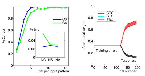
Example simulation of general structure model. Left panel: model performance on transfer task. Qualitative results are similar to C-TS model predictions. Right panel: average attentional weights. During the training phase, no structure is a better predictor of outcomes. However, the model infers the C-TS structure over the test phase.

We proposed a high level model to study the interaction of cognitive control and learning of context-task-set hidden structure, and for re-using this structure for generalization. This model does not however address the mechanisms that support its computations (and hence it does not consider whether they are plausibly implemented), nor does it consider temporal dynamics (and hence reaction times). In the next section, we propose a biologically detailed neural circuit model which can support, at the functional level, an analogous learning of higher and lower level structure using purely reinforcement learning. The architecture and functionality of this model is constrained by a wide range of anatomical, physiological data, and it builds on existing models in the literature. We then explore this model’s dynamics and its internal representations, and relate them to the hidden structure model described above. This allows us to make further predictions for human behavioral experiments described thereafter.

4 Neural network implementation

Our neural model builds on an extensive literature of the mechanisms of gating of motor and cognitive actions and reinforcement learning in corticostriatal circuits, extended here to accommodate hidden structure. We first describe the functionality and associated biology in terms of a single corticostriatal circuit for motor action selection, before discussing extensions to structure building and task-switching. All equations can be found in the appendix.

In these networks, the frontal cortex “proposes” multiple competing candidate actions (e.g., motor responses), and the basal ganglia selectively gates the execution of the most appropriate response via parallel re-entrant loops linking frontal cortex to basal ganglia, thalamus and back to cortex (Alexander & DeLong, 1986; Mink, 1996; Frank & Badre, 2011). The most appropriate response for a given sensory state is learned via dopaminergic reinforcement learning signals (Montague et al., 1996) allowing networks to learn to gate responses that are probabilistically most likely to produce a positive outcome and least likely to lead to a negative outcome (Doya, 2002; Houk, 2005; Frank, 2005; Maia, 2009; Dayan & Daw, 2008). Notably, in the model proposed below, there are two such circuits, with one learning to gate an abstract task-set (and to cluster together contexts indicative of the same task-set), and the other learning to gate a motor response conditioned on the selected task-set and the perceptual stimulus. These circuits are arranged hierarchically, with two main “diagonal” frontal-BG connections from the higher to the lower loop striatum and subthalamic nucleus. The consequences are that: (i) motor actions to be considered as viable are constrained by task-set selection; (ii) conflict at the level of task-set selection leads to delayed responding in the motor loop, preventing premature action selection until the valid task-set is identified. As we show below, this mechanism not only influences local within-trial RTs, but also renders learning more efficient across trials by effectively expanding the state space for motor action selection and thereby reducing interference between stimulus-response mappings across task-sets.

The mechanics of gating and learning in our specific implementation (Frank, 2005, 2006) are as follows (described first for a single motor loop). Cortical motor response units are organized in terms of “stripes” (groups of interconnected neurons that are capable of representing a given action; see Figure 3). There is lateral inhibition within cortex, thus supporting competition between multiple available responses (e.g. Usher & McClelland, 2001). But unless there is a strong learned mapping between sensory and motor cortical response units, this sensory-to-motor cortico-cortical projection is not sufficient to elicit a motor response, and alternative candidate actions are all noisily activated in PMC with no clear winner. However, motor units within a stripe also receive strong bottom-up projections from, and send top-down projections to, corresponding stripes within the motor thalamus. If a given stripe of thalamic units becomes active, the corresponding motor stripe receives a strong boost of excitatory support relative to its competitors, which are then immediately inhibited via lateral inhibition. Thus, gating relies on selective activation of a thalamic stripe.

Figure 3. Neural network models.

Top: Schematic representation of a single loop corticostriatal network. Here, input features are represented in two separate input layers. Bottom: schematic representation of the two loop corticostriatal gating network. Color context serves as input for learning to select the TS in the first PFC loop. The PFC TS representation is multiplexed with the shape stimulus in the parietal cortex, the representation of which acts as input to the second motor loop. Before the TS has been selected, multiple candidate TS representations are active in PFC. This TS-conflict results in greater excitation of the subthalamic nucleus in the motor loop (due to a diagonal projection), thus making it more difficult to select motor actions until TS conflict is resolved. PMC: Premotor cortex; STN: subthalamic nucleus; Str: Striatum; Thal: Thalamus; GPe: Globus Pallidus external segment; GPi: Globus Pallidus internal segment.

Critically, the thalamus is under inhibition from the output nucleus of the basal ganglia, the globus pallidus internal segment, GPi. GPi neurons fire at high tonic rates, and hence the default state is for the thalamus to be inhibited, thereby preventing gating. Two opposing populations of neurons in the striatum contribute positive and negative evidence in favor of gating the thalamus. These populations are intermingled and equally represented, together comprising 95% of all neurons in the striatum (Gerfen & Wilson, 1996). Specifically, the “Go” neurons send direct inhibitory projections to the GPi. Hence, Go activity in favor of a given action promotes inhibition and disinhibition of the corresponding stripes in GPi and thalamus respectively, and hence gating. Conversely, the “NoGo” neurons influence the GPi indirectly, via inhibitory projections first to the external segment of the globus pallidus (GPe), which in turn tonically inhibits GPi. Thus, whereas Go activity inhibits GPi and disinhibits thalamus, NoGo activity opposes this effect. The net likelihood of a given action to be gated is then a function of the relative difference in activation states between Go and NoGo populations in a stripe, relative to that in other stripes.

The excitability of these populations are dynamically modulated by dopamine: whereas Go neurons express primarily D1 receptors, NoGo neurons express D2 receptors, and dopamine exerts opposing influences on these two receptors. Thus, increases in dopamine promote relative increases in Go vs. NoGo activity, whereas decreases in dopamine have the opposite effect. The learning mechanism leverages this effect: positive reward prediction errors (when outcomes are better than expected) elicit phasic bursts in dopamine, whereas negative prediction errors (worse than expected) elicit phasic dips in dopamine. These dopaminergic prediction error signals transiently modify Go and NoGo activation states in opposite directions, and these activation changes are associated with activity-dependent plasticity, such that synaptic strengths from corticostriatal projections to active Go neurons are increased during positive prediction errors, while those to NoGo neurons are decreased, and vice-versa for negative prediction errors. These learning signals increase and decrease the probability of gating the selected action when confronted with the same state in the future.

This combination of mechanisms has been shown to produce adaptive learning in complex probabilistic reinforcement environments using solely reinforcement learning (e.g. Frank, 2005). Various predictions based on this model, most notably using striatal dopamine manipulations, have been confirmed empirically (see e.g., Maia & Frank (2011) for recent review). Moreover, an extension of the basic model includes a third pathway involving the subthalamic nucleus (STN), a key node in the BG circuit. The STN receives direct excitatory projections from frontal cortical areas and sends direct and diffuse excitatory projections to the GPi. This ‘hyperdirect’ pathway bypasses the striatum altogether, and in the model supports a ‘global NoGo’ signal which temporarily suppresses the gating of all alternative responses, particularly under conditions of cortical response conflict (Frank (2006); see also Bogacz (2007)). This functionality provides a dynamic regulation of the model’s decision threshold as a function of response conflict (Ratcliff & Frank, 2012), such that more time is taken to accumulate evidence among noisy corticostriatal signals to prevent impulsive responding and to settle on a more optimal response. Imaging, STN stimulation, and electrophysiological data combined with behavior and drift diffusion modeling are consistent with this depiction of frontal-STN communication (Aron et al., 2007; Frank et al., 2007a; Wylie et al., 2010; Isoda & Hikosaka, 2008; Cavanagh et al., 2011; Zaghloul et al., 2012). Below we describe a novel extension of this mechanism to multiple frontal-BG circuits, where conflict at the higher level (e.g. during task-switching) changes motor response dynamics.

4.1 Base network - No structure

We first apply this single corticostriatal circuit to the problems simulated in the more abstract models above (Fig 3, top). Here, the loop contains two input layers, encoding separately the two input dimensions (eg. color and shape). The premotor cortex layer contains four stripes, representing four motor actions available. Each premotor stripe projects to a corresponding striatal ensemble of 20 units (10 Go and 10 NoGo) encoding a distributed representation of input stimuli, and which learn the probability of obtaining (or not obtaining) a reward if the corresponding action is gated. Input-striatum weights are initialized randomly, while input projections to premotor cortical (PMC) units are uniform. Only input-striatum synaptic weights are plastic (subject to learning) (see appendix for weight update equations). This network is able to learn all basic tasks presented using pure reinforcement learning (i.e. using only simulated changes in dopamine, without direct supervision about the correct response) in very efficient time. However, it has no mechanisms for representing hidden structure and is thus forced to learn in a ‘flat’ way, binding together the input features, similar to the flat computational model. Thus it should not show evidence of transfer or structure in its pattern of errors or RTs.

4.2 Hidden structure network

We thus extended the network to include two nested corticostriatal circuits. The anterior circuit initiates in the prefrontal cortex (PFC), and actions gated into PFC provide contextual input to the second posterior premotor cortex (PMC) circuit (fig 3 bottom, fig 4). The interaction between these two corticostriatal circuits is in accordance with anatomical data showing that distinct frontal regions project preferentially to their corresponding striatal region (at the same rostrocaudal level), but that there is also substantial convergence between loops (see Haber, 2003; Calzavara et al., 2007; Draganski et al., 2008; Nambu, 2011). Moreover, this rostrocaudal organization at the level of corticostriatal circuits is a generalization of the hierarchical rostrocaudal organization of the frontal lobe (Koechlin et al., 2003; Badre, 2008). A related neural network architecture was proposed in Frank & Badre (2011), but we modify it here to accommodate hidden structure, to include BG gating dynamics including the STN and GP layers, and pure reinforcement learning at all levels.⁴

Figure 4. Neural network model.

Top: Detailed representation of the two-loop network. See text for detailed explanation of connectivity and dynamics. Parametrically manipulated projection strengths are highlighted: (1) connectivity between color input and PFC (fully connected vs. one-to-one organized C-PFC mapping, which increases the likelihood that the network assigns distinct PFC states to distinct contexts); (2) STN to GPi strength (modulating the extent to which motor action selection is inhibited given conflict at the level of PFC task-set selection); (3) diagonal PFC to pStr connection strength (modulating task-set motor action preparation); (4) pStr learning rate. PFC: Prefrontal cortex; PC: Parietal cortex; PMC: Premotor cortex; STN: subthalamic nucleus; Str: Striatum; Thal: Thalamus; GPe: Globus Pallidus external segment; GPi: Globus Pallidus internal segment; SNc: Substancia nigra pars compacta. a and p indicate anterior and posterior loops. Bottom Example of the time course of PFC activations (for chosen and other TS), average STN activity and chosen motor output unit activity in correct stay and switch trials. In switch trials, co-activation of PFC stripes results in stronger STN activation, thus preventing action selection in the motor loop until conflict is resolved, leading to increased reaction times.

As in the Bayesian C-TS model, we do not consider here the learning of which dimension should act as context or stimulus, but assume they are given as such to the model and investigate the consequential effects on learning. We extend and discuss this point further down in the paper. Thus, only the context (eg. color) part of the sensory input projects to PFC, whereas the stimulus (eg. shape) projects to posterior visual cortex. The stimulus representation in parietal cortex (PC) is then contextualized by top-down projections from PFC. Weights linking the shape stimulus inputs to parietal cortex are predefined and organized (top half of layer reflects shape 1 and bottom half shape 2). In contrast, projections linking color context inputs to PFC are fully and randomly connected with all PFC stripes, such that PFC representations are not simply frontal “copies” of these contexts; rather they have (initially) no intrinsic meaning, but as we shall see, come to represent abstract states that contextualize action selection in the lower motor action selection loop.

There are three PFC stripes, each subject to gating signals from the anterior striatum, with dynamics identical to those described above for a single loop – but with PFC stripes reflecting abstract states rather than motor responses. When a PFC stripe is gated in response to the Color context, this PFC representation is then multiplexed with the input Shape stimulus in the parietal cortex (PC), such that PC units contain distinct representations for the same sensory stimulus in the context of distinct (abstract) PFC representations (Reverberi et al., 2011). Specifically, while the entire top half (all three columns) of the PC layer represents shape 1 and the bottom half shape 2, once a given PFC stripe is gated, it provides preferential support to only one column of PC units (and the others are suppressed due to lateral inhibition). Thus the anterior BG-PFC loop acts to route information about a particular incoming stimulus to different PC “destinations”, similar to a BG model proposed by Stocco et al. (2010). In our model, the multiplexed PC representation then serves as input to the second PMC loop for motor action selection. The PMC loop contains 4 stripes, corresponding to the 4 action choices, as in the single circuit model above.

Dopaminergic reinforcement signals modify activity and plasticity in both loops. Accordingly, the network can learn to select the most rewarding of four responses but will do so efficiently only if it also learns to gate the different input Color contexts to two different PFC stripes. Note, however, that unlike for motor responses, there is no single a priori “correct” PFC stripe for any given context – the network creates its own structure. Heuristically, PFC stripes represent the hidden states the network gradually learns to gate in response to contexts. The PMC gating network learns to select actions for a stimulus in the context of a hidden state (via their multiplexed representation in parietal cortex), thus precisely comprising the definition of a task-set. Consequently, this network contains a higher level PFC loop allowing for the selection of task-sets (conditioned on contexts, with those associations to be learned), and a lower level MC loop allowing for the selection of actions conditioned on stimuli and the PFC-task-sets (again with learned associations). In accordance with the role of PFC for maintaining task-set in working memory, we allow PFC layer activations to persist from the end of one trial to the beginning of the next.

4.2.1 Cross-loop “diagonal” projections

We include two additional new features to the model whereby the anterior loop communicates along “diagonal” projections with the posterior BG (Nambu, 2011, e.g.,). First, it is important that motor action gating in the second loop does not occur before the task set has been gated in the first loop. Indeed, this would lead to action selection according only to stimulus, neglecting task-set. This is accomplished by incorporating the STN role as implemented in Frank (2006), but here where STN in the motor loop detects conflict in PFC from the first loop, instead of just conflict between alternative motor responses. Indeed, PFC to STN projection is structured in parallel stripes, so that coactivation of multiple PFC stripes elicits greater STN activity, and thus a stronger global No-Go signal in the GPi. Thus, early during processing, when a task-set has not yet been selected, there is co-activation between multiple PFC stripes, and gating of motor actions is prevented by the STN until conflict is resolved in the first loop (i.e., a PFC stripe has been gated). See specific dynamics in figure 4, bottom.

Second, we also include a diagonal input from the PFC to the striatum of the second loop, thereby contextualizing motor action selection according to cognitive state (see also Frank & Badre, 2011). This projection enables a task-set preparatory effect: the motor striatum can learn associations from the selected PFC task-set independently of the lower level stimulus, thus preferentially preparing both actions related to a given task-set. As discussed earlier, these features are in accordance with known anatomy: indeed, although the cortico-basal ganglia circuits involve parallel loops, there is a degree of transversal overlap across parallel loops, as required by this diagonal PFC-lower loop striatum projection, as well as influence of first loop conflict on second loop STN (Draganski et al., 2008).

It should be emphasized that the tasks of interest are expected to be difficult to learn by such a structured network without explicit supervision and using only reinforcement learning across 4 motor responses, especially due to credit assignment issues. Indeed, initially, both TS and action gating are random. Thus, feedback is ambiguously applied to both loops: an error is interpreted both as an inappropriate TS selection to the color context and incorrect action selection in response to the shape stimulus within the selected TS. However, this is the same problem faced by human participants, who do not receive supervised training and have to learn on their own how to structure the representations.

5 Neural network results

Although such networks include a large number of parameters pertaining to various neurons’ dynamics and their connectivity strengths, the results presented below are robust across a wide range of parameter settings. We validate this claim below.

5.1 Neural network simulations: initial clustering benefit

As for the C-TS model, we first assess the neural network’s ability to cluster contexts onto task-sets when doing so provides an immediate learning advantage. We do so in a minimal experimental design permitting assessment of the critical effects. We ran 200 networks, from which 3 were removed from analysis due to outlier learning. Simulation details are found in appendix and figure 5.

Figure 5. Neural Network Simulation 1.

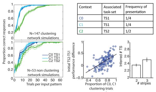
Top Right: Experimental design summary Left Learning curves for different conditions. Top: 75% of networks adequately learned to select a common PFC representation for the two contexts corresponding to the same rule, and thus learned faster (clustering networks). Bottom: the remaining 25% of the networks created two different rules for C0 and C1, and thus showed no improved learning. Bottom Middle Performance advantage for the clustering networks was significantly correlated with the proportion of trials in which the network gated the common PFC representation. Bottom Right Quantitative fits to network behavior with the C-TS model showed a significant increase in inferred number of hidden TS for clustering compared to non-clustering simulations.

Rapid recognition of the fact that two contexts C0 and C1 are indicative of the same underlying TS should permit the ability to generalize stimulus-response mappings learned in each of these contexts to the other. As such, if the neural network creates one single abstract rule that is activated to both C0 and C1, we expect faster learning in contexts C0 and C1 than in C2, which is indicative of a different TS. Indeed, figure 5 (left) shows that the network’s learning curves were faster for C0 and C1 than they are for C2 (initial performance on first 15 trials of all stimuli: t = 7.8 ; p < 10⁻⁴).

This performance advantage relates directly to identifying one single hidden rule associated to contexts C0 and C1. Because the network is a process model, we can directly assess the mechanisms that give rise to observed effects. For each network simulation, we determined which PFC stripe is gated in response to contexts C0, C1 and C2 (assessed at the end of learning, during the last 5 error-free presentations of each input). All networks selected a different stripe for C2 than for C1 and C0, thus correctly identifying C2 as indicative of a distinct task-set. Moreover, 75% of networks (147) learned to gate the same stripe for C0 and C1, correctly identifying that these corresponded to the identical latent task-set. The remaining 25% (50) selected two different stripes for C0 and C1, thus learning their rules independently – that is, like a flat model.

Importantly, the tendency to cluster contexts C0 and C1 into a single PFC stripe was predictive of performance advantages. Learning efficiency in C0/C1 was highly significantly improved relative to context C2 for the clustering networks (figure 5 top left, N = 147; t = 9.4 ; p < 10⁻⁴) whereas no such effect was observed in non-clustering networks (figure 5 bottom left, N = 50; t = 0.3; p = 0.75). Directly contrasting these networks, clustering networks performed selectively better than non-clustering networks in C0/C1 (t = 4.9; p < 10⁻⁴), with no difference in C2 (t = −0.94; p = 0.35).

Within the clustering networks, we compute the proportion of trials in which the network gated the common stripe for TS1 in contexts C0 and C1, as a measure of efficiency in identifying a common task-set. This proportion correlated significantly with the increase in C0/C1 performance (figure 5 bottom middle, r = 0.72 ; p < 10⁻⁴), with no relation to C2 performance (r = −0.01; p = 0.89).

5.2 Neural network simulations: structure transfer

5.2.1 Neural network dynamics lead to similar behavioral predictions as C-TS model

This second set of simulations investigate structure transfer after learning, as described above for the C-TS model. Recall that these simulations include two consecutive learning phase, labeled training phase followed by a test phase. During the training phase, interleaved inputs include two contexts (C1 and C2) and two stimuli (S1 and S2). During the test phase, new contexts are presented to test transfer of a previously used TS (C3-Transfer), or learning of a new TS (C4-new).

The two-loop nested network was able to learn the task, with mean time to criterion 22.1(±2.6) repetitions of each of the four inputs.⁵

Moreover, as in the C-TS model, a clear signature and potential advantage of structure became clear in the test phase. First, learning was significantly faster in the C3 transfer condition than in the C4-new condition, thus positive transfer (fig 6a). Second, the repartition of error types was similar to that expected by the C-TS model (and as we shall see below, exhibited by human subjects). In particular, the network exhibited more errors corresponding to the wrong TS selection (NC) than other errors, especially in the new condition (figure 6i). As explained earlier, this is a sign of negative transfer – the tendency to reapply previous task-sets to situations that ultimately require creating new task-sets.

Figure 6. Neural network results.

Top a-c): test phase results, for Transfer (blue), New-overlap (green) and New-incongruent (red) conditions. Left: Proportion of correct trials as a function of input repetitions, inset: proportion of NC, NS and NA errors. Positive transfer is visible in the faster Transfer than New learning curves; Negative transfer is visible in the interaction between condition and error types and in the slower slope in New-overlap than New-Incongruent conditions. Right: Proportion of task-set TS1 (b), and blank TS (c) hidden state selections as a function of trials, for all conditions. Positive transfer is visible in the reuse of TS1 stripe in the transfer condition, and negative transfer in the reduced recruitment of the new TS stripe for new-overlap compared to new-incongruent conditions. Bottom: Asymptotic learning phase results. d): reaction-time switch-cost; e) error type and switch effects on error proportions. f): slower reaction-times for neglect L than neglect H errors.

To further investigate the source of negative transfer, we also tested networks with a third test condition, “C5-new-incongruent”, which was new but completely incongruent with previous stimulus response associations. While both C4 and C5 involved learning new task-sets, in the C5 test-condition the task-set did not overlap at all with the two previously learned task-sets: if either was gated into PFC, it led to incorrect action selection for both stimuli. This situation contrasts with that for C4, in which application of either of the previous task-sets leads to correct feedback for one stimulus and incorrect for the other, making inference about the hidden state more difficult. Indeed, networks were better able to recruit a new stripe in the C5 compared to C4 test condition (p < 0.02, t > 2.4, fig 6 b, c), leading to more efficient learning. Although initial performance was better in the C4 overlap condition (t = 3.7, p = 5 10⁻⁴, fig 6a), due to the 0.5 probability of reward resulting from selection of a previous task-set, subsequent learning curves were steeper in the C5 condition, due to faster identification of the necessity for a new hidden state.

Again, we can directly assess the mechanisms that give rise to these effects. Similarly to the previous simulations, for each network simulation, we determined which PFC stripe is gated in response to contexts C1 and C2 at the end of learning, corresponding to TS1 and TS2. We then assessed during the test phase which of the three stripes was gated for each transfer condition.

This analysis largely confirmed the proposed mechanisms of task-set transfer. In the C3 transfer condition (fig 6b), more than 70% of the networks learned to reselect stripe TS1 in response to the new context, thus transferring TS1 stimulus-action associations to the new situation, despite the fact that the weights from the units corresponding to C3 were initially random. The remaining 30% of networks selected the third previously unused (“blank”) TS stripe, and thus relearned the task-set as if it were new. In contrast, in the C4 new test condition (fig 6c), ≈90% of networks appropriately learned to select the blank TS stripe. The remaining 10% of networks selected either the TS1 or TS2 stripes, due to overlap between these task-sets and the new one, leading to negative transfer. In this small number of cases, rather than creating a new task-set networks simply learned to modify the stimulus-action associations linked to the old task-set; eventually performance converged to optimal in all networks.

To confirm the presumed link between the generalization advantage in the C3 transfer condition and the gating of a previously learned task-set, we investigated the correlation between performance and the proportion of blank TS stripe selection. This analysis was conducted over the wide array of simulations, including those designed to explore the robustness of the parameter space (fig 7). The selection of the blank stripe was highly significantly (both p’s < 10⁻¹³) anti-correlated with C3 transfer performance (r = −0.11), and positively correlated with C4 new-overlap performance (r = 0.55).⁶

Figure 7. Neural Network parameter robustness.

Exploration of systematic modulations of key network parameters across a wide range. For each parameter, the significance values are plotted for each of five main behavioral effects (see descriptions in main text), from top to bottom: 1) Transfer versus new-overlap performance difference; 2) asymptotic learning phase error repartition effect; 3) asymptotic learning phase error reaction times NH < NL; 4) Test-phase old > new PFC stripe selection for the transfer condition; 5) Test phase new > old PFC stripe selection for the new condition. Simulations were conducted 100 times each, in each case with the other 4 parameters fixed to the corresponding white bar value, and 1 parameter varied along a wide range. 1st line: Cortico-striatal learning rate (here fixing learning rates to be the same for both loops); 2nd line: motor-cortex striatum learning rate; 3rd line: PFC-striatum learning rate; 4th line: Diagonal PFC-posterior striatum relative projection strength; 5th line: STN to 2nd loop GPi relative projection strength. Results across all five effects were largely robust to parameter changes.

Thus, these first analyses show that the neural network model creates and re-uses task-sets linked to contexts as specified by the high level C-TS computational model. Below we provide a more systematic and quantitative analysis showing how each level of modeling relates to the other. But first, we consider behavioral predictions from the neural model dynamics.

5.2.2 Neural network dynamics lead to behavioral predictions: switch costs, RTs, and error repartition

While we have shown that the neural network affords similar predictions as the C-TS structure learning model, in terms of positive and negative transfer, it also allows us to make further behavioral predictions most notably related to dynamics of selection. We assess these predictions during the asymptotic learning phase.

The persistence of PFC activation states from the end of one trial to beginning of next (a simple form of working memory), resulted in performance advantage for task-set repeat trials, or conversely, a switch-cost, with significantly more errors (fig 6e) and slower reaction times (fig 6d) in switch trials. This is because in a switch trial, gating of a different PFC stripe than that in the previous trial took longer than simply keeping the previous representation active. This longer hesitation in PFC layer led to three related effects.

First, it initially biased the PC input to the second loop to reflect the stimulus in context of the wrong task-set, thus leading to an increased chance of an error if the motor loop responds too quickly, and hence an accuracy switch-cost (and a particular error type).

Second, when the network was able to overcome this initial bias and respond correctly, it was slower to do so (due to the additional time associated with updating the PFC task-set and then processing the new PC stimulus representation), and hence a reaction-time switch-cost.

Third, and counter-intuitively, the error repartition favored NS errors over NC errors, over NA errors (fig 6e). This pattern arose because the hierarchical influence of PFC onto posterior (motor) striatum led to a task-set preparatory effect, where the two actions associated with the TS were activated before the stimulus was itself even processed. Thus, actions valid for the task-set (but not necessarily the stimulus) were more likely to be gated than other actions, leading to more NS errors. In contrast, NC errors resulted from impulsive action selection due to application of the previous trial’s task-set (particularly in switch trials). Indeed, during switch trials, error reaction-times were significantly faster for NC errors than NS errors (fig 6f). If these dynamics are accurate, we thus predict a very specific pattern of errors by the end of the learning phase:

• presence of an error and reaction time switch cost when c_t ≠ c_t+1, but not s_t ≠ s_t+1

• prevalence of within task-set errors (neglect of the stimulus), rather than perseveration errors (neglect of the context) on switch trials

• faster within than across task-sets errors

We also ensured that all the behavioral predictions are robust to parameter manipulation of the network. In particular, we show in figure 7 that the majority of predicted effects hold across systematic variations in key parameters, including corticostriatal learning rates and connection strengths between various layers, including PFC-striatum and STN-GPi. The main results presented above were obtained with parameters representative from this range.

6 Linking levels of modeling analysis

In this section we show that the approximate Bayesian C-TS formulation provides a good description of the behavior of the network, and moreover, that distinct mechanisms with the neural model correspond to selective modulation of parameters within the higher level model. To do so, we quantitatively fit the behavior generated by the neural network simulations (including both experimental protocols) with the C-TS, by optimizing the parameters of the latter model that maximizes the log likelihood of networks’ choices given the history of observations Frank & Badre (2011). Parameters optimized include the clustering parameter α, the initial Beta prior strength on task-sets n₀ (potentially reported as i₀ = 1/n₀ for a positively monotonous relationship with a learning rate equivalent), and a general action selection noise parameter, the softmax β. For comparison, we also fit a flat model, including parameters n₀ and β, taking model complexity into account by evaluating fits using the Akaike Information Criterion (AIC; Akaike, 1974), as well as exceedance probability on AIC (Stephan et al., 2009).

6.1 Simulation 1: Initial clustering benefit

First, the C-TS structure model fit the networks’ behavior significantly better than a flat model (t = 5.45; p < 10⁻⁴, exceedance probability p = 0.84), for both clustering networks (t = 5.06; p < 10⁻⁴) and non-clustering networks (t = 2.17; p = 0.035), with no significant difference in fit improvement between groups (t = 0.49, ns).⁷ Correlation between empirical and predicted probabilities choice (grouped in deciles) over all simulations was high: r² = 0.965, p < 10⁻⁴. Mean pseudo-r² value comparing the likelihood of the precise sequence of individual trials to chance was also strong, at 0.46.

Given that the fits were reasonable, we then assessed the degree to which network tendencies to develop a clustered gating policy corresponded to inferred number of task-sets from the C-TS structure model. If a gated PFC stripe corresponds to use of an independent task-set, then the clustering networks (which by definition use fewer PFC stripes) should be characterized by lower inferred number of latent task-sets in the fits. As expected, the inferred number of task-sets was significantly lower for the clustering networks compare to non-clustering ones (figure 5 bottom right, t = 2.28, p = 0.023). Within the clustering networks, the proportion of common final TS1 stripe use for C0 and C1 was significantly correlated with the fitted number of task-sets inferred by the models (p = 0.027, r = −0.18).

Notably, there were no differences in the prior clustering parameter α across the two groups of networks, as expected from their common initial connectivity structure. Rather, differences in clustering were produced by random noise and choices leading to different histories of action selection which happen to sometimes reinforce a common stripe gating policy or not. Due to its approximate inference scheme, C-TS is also sensitive to specific trial order. We investigate systematically the effect of priors below by manipulating the connectivity. The fact that the hidden structure C-TS model can detect these differences in clustering due to specific trial history (without having access to the internal PFC states) provides some evidence that the two levels of modeling use information in similar ways for building abstract task-sets while learning from reinforcement. This claim is reinforced by subsequent simulations below.

6.2 Simulation 2: Structure transfer

We applied the same quantitative fitting of network choices with the C-TS model for the second set of simulations for the structure transfer task. Again, the C-TS structure model fits better than a at model, penalizing for model complexity (t = 5:8, p < 10⁻⁶, true for 46 out of 50 simulations, exceedance probability p = 1:0). Moreover, these fits indicated that networks were likely to re-use existing task-sets in the C3 transfer condition, whereas networks were more likely to create a new task-set in C4 and C5. Indeed, the inferred number of additional task-sets created in the transfer phase (beyond the two created for all simulations during the learning phase), was E(N) = 0:05 for C3 vs 0:84 for C4; p < 10⁻⁴ ; t = −13:8). Networks were even more likely to create a new task-set for the C5 new-incongruent condition (E(N) = 0.99; significantly greater than C4; p = 0.0009 ; t = −3.53).

Together with the previous simulation, this result establishes a link between the gating of a PFC stripe – with no initial meaning to that stripe – to the creation (or re-use) of a task-set, as formalized in the C-TS model. The C-TS model has no access to the latent PFC states of the network, but based on the sequence of choices can appropriately infer the number of stripes used. A strong prediction of this linking is that if we do give access to the C-TS model of the PFC state selected by the network in individual trials, the fit to network choices should improve. Indeed, model fits improved significantly when we condition predicted choice probabilities not only on the past sequence of inputs, action choices and rewards (as is typically done for RL model fits to human subjects), but also on the sequence of model-selected PFC stripes (p = 0.0025 ; t = −3.2). The reason for this improvement is that when the network gates an unexpected PFC stripe (which can happen due to network dynamics including random noise), the predicted motor response selected by the network now takes into account the corresponding TS, thus allowing the model fits to account for variance in types of errors.

6.3 Parametric manipulations on NN mechanisms are related to parametric influences on specific C-TS model computations

Thus, we have shown the C-TS model can mimic functionality of the nested corticostriatal circuit. This analysis provides the basis for exploring whether and how specific mechanisms within the neural model give rise to the higher level computations. To do so, we parametrically manipulated specific neural model parameters and studied their impact on both behavior and the fitted parameters within the C-TS model framework.

We report below the links investigated, but refer the readers to the appendix for a more detailed analysis.

1. PFC-STN diagonal projection: conditionalizing actions by task-sets. A fundamental aspect of the C-TS model is that action values are conditionalized not only by the stimulus but by the selected higher level task-set choice Q(s, a_k) = E(r∣s_t, a_k, TS_t). When implemented in a dynamic process model, how does the lower level corticostriatal motor loop ensure that its action values are properly contextualized by TS selection? As described earlier, the diagonal projection from PFC to motor-STN is critical for this function, preventing premature responding before task-sets are selected and shaping the structure that is learned. In particular, when the STN is lesioned in the network, learning is slowed to 37 ± 2.3 input iterations to criterion (as opposed to 22.1 ± 2.6 with the STN (see appendix). To investigate this effect we parametrically manipulated the efficacy of STN projections and examined its effect on fitted C-TS model parameters. We predicted that STN efficacy would affect the reliability of task-set selection (i.e. lower STN projection strengths would lead to ignorance of the selected task-set during motor action selection). Indeed, we observed a strong correlation between neural network STN projection strength and fitted parameter β_TS (figure 8 left, r = 0.62, p = 0.01), but no effect on other parameter values (r < 0.33, p > 0.2) . That is, despite the fact that STN strength influences learning speed, the C-TS model recovers this effect by correctly assigning it to variance in task-set selection and hence more interference in learning, rather than in learning rate or in noise in motor action selection.

2. PFC-striatum diagonal projection: task-set action preparation. Similarly, the C-TS model proposes that once a TS is selected, the available actions are constrained by that TS, such that any errors are more likely to compose of within-TS errors (actions that are valid for that TS but ignoring the lower level stimulus). We investigated how the PFC-motor striatum diagonal projection is involved in preparing actions according to the selected task set, and hence can lead to errors of this type. Indeed, parametric manipulations of the strength of this projection yielded a very strong correlation with the fitted within-TS noise parameter ∊_TS (r = 0.97, p = 3.10⁻⁴, figure 8 right). Thus PFC biasing of motor striatum increases action preparation within task-sets, leading to a specific type of error, namely those associated with neglecting the stimulus (NS errors).⁸

3. Organization of context to PFC projections: clustering. Another key component within the C-TS model is the tradeoff in the decision of whether to build a new TS when encountering a new context, or whether to cluster it into an existing TS. In the neural network, the tendency to activate a new PFC state or re-use an existing one can be altered by varying the organization of projections from the context layer to PFC. We parametrically manipulated the connectivity from contextual inputs to PFC, from full-random connectivity (enabling clustering by allowing multiple contexts to activate common PFC representations) to one-to-one (where networks are encouraged to represent distinct contexts in distinct PFC stripes)⁹. We hypothesized that differential scaling of these two connectivities would modulate the tendency to cluster contexts and hence correspond to an effect on the α clustering parameter in the C-TS model fits. Indeed, fig 9 shows that stronger priors were associated with a greater tendency to select the new stripe in the transfer test conditions (r = 0.68, p = 0.001, fig 9 bottom), which coincides with a decrease in transfer performance (r = −0.59, p = 0.007, fig 9 top), and increase in new-overlap performance (r = 0.86, p < 10⁻⁴, fig 9 top). This effect on transfer performance is analogous to the result displayed earlier with the C-TS computational model, in which we found a similar relationship with Dirichlet α (fig 2). Thus, as predicted, we observed a strong correlation between the network manipulated parameter and C-TS fitted α (r = 0.76, p < 2.10⁻⁴, figure 8 middle left). Multivariate linear regression of network parameter against fitted parameters showed that only Dirichlet α accounted significantly for the variability.

4. Motor corticostriatal learning rate: stimulus-action learning. Finally, the C-TS model includes a free parameter n₀ affecting the degree to which stimulus-action associations are updated by new outcome information. In the neural model this corresponds to the learning rate within the lower motor corticostriatal projections. We thus parametrically manipulated this learning rate and assessed the degree to which it affected the recovered n₀ parameter. Multivariate linear regression of network learning rate against the four fitted parameters showed that only n₀ accounted significantly for the variability. More specifically, we looked at i₀ = 1/n₀ as a marker of learning speed, and found a significant positive correlation between fit i₀ and motor striatal learning rate (r = 0.85, p = 0.0008, figure 8 middle right). This contrasts with the above effects of STN strength, which affected overall learning speed without impacting the learning rate parameter, due to its modulation of structure and interference across task-sets.

Figure 8. Linking corticostriatal neural network to C-TS model.

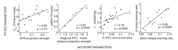
Mean C-TS fitted parameters are plotted against manipulated neural network parameters used for corresponding simulations. Diagonal PFC-STN projection strength was related to noise in TS selection; diagonal PFC-striatum was related to within-TS noise. C-PFC connectivity was related to clustering prior; Motor striatal learning rate was related to action learning rate parameter.

Figure 9. Effects of context-PFC prior connectivity.

50 neural network simulations per C-PFC prior parameter value. The C-PFC parameter scales the weight of the organized (one-to-one) context input to task-set PFC layer projection relative to the fully connected uniform projection. a) Mean (standard error) performance and b) Proportion of new stripe selection on the transfer (blue) and new-overlap (green) test conditions as a function of C-PFC prior parameter. The stronger the prior for one-to-one connectivity, the more likely the network is to select a new stripe for new contexts 50 in the test phase, thereby suppressing any difference in performance between the three test conditions. Conversely, a greater ability to arbitrarily gate contexts into PFC stripes allows networks to re-use stripes when appropriate.

In summary, the fittings described in this section revealed that the C-TS model can be approximately implemented in a nested two-loop cortico-basal gating neural network. Although we do not argue that the two levels of modeling execute the exact same computations (see discussion), we argue that the neural network represents a reasonable approximate implementation of the formal information manipulations executed by the high level computational model. Indeed both levels of modeling behave similarly at the action selection level, as shown by similar qualitative predictions and by quantitative fits. Fits also reveal a good concordance between hidden variables manipulated by the functional model (abstract task-sets), and their equivalents in the neural network model (abstract prefrontal stripes). Finally, these simulations verified that the fitting procedure can appropriately recover parameters such as α for simulated subjects in which we explicitly manipulate the likelihood of visiting new TS states.

The two levels of modeling make distinct but concordant predictions about the nature and dynamics of task-set selection and switching. In the following section we present two behavioral experiments designed to test some of these predictions.

7 Experiments

The models make a key prediction that subjects conditionalize action selection according to task-sets, and that a predisposition to use this strategy may exist even when it is not immediately necessary, as revealed in various measures of transfer and error repartition. The reasoning for this possibility is discussed in the introduction. We thus tested this prediction by using the structure transfer paradigm simulated by the models above, in which there is no immediate advantage to creating and learning structure. In the following, we first describe the precise experimental procedure, then summarize the models’ predictions and develop alternative models predictions, then present experimental results and model fits validating our theory.

7.1 Experimental paradigm: Experiment 1

The experiment (Fig 10) consisted of two sequential learning phases. Both phases required learning correct actions to two-dimensional stimuli from reinforcement feedback, but for convenience we refer to the first phase as the learning phase and the second phase as the test phase. The first phase was designed such that there would be no overt advantage to representing structure in the learning problem. The second test phase was designed such that any structure built during learning would facilitate positive transfer for one new context, but negative transfer for another. Note also that we define these phases functionally for the purpose of the experimental analysis; to the subject these phases transitioned seamlessly one after the next with no break or notification.

Figure 10. Experimental protocol.

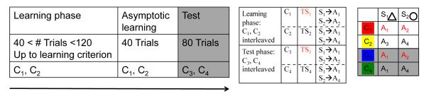
Left: experimental phases. The learning phase is comprised of pseudo-randomly intermixed colored shapes (in this example), comprising shapes S1 and S2, and colors C1 and C2. Each input combination is presented up to a fixed learning criterion, followed by a 10 trial (per input) asymptotic learning phase. Next, the test phase comprises 20 trials per four new inputs, comprising previous shapes in new colors. There is no break in between phases. Middle: Correct input-action associations. Right: Example of correct input-action associations with colors and shapes as context and stimuli. Note that correct actions for red shapes in the learning phase can be re-applied to the blue shapes in the test phase. Thus we refer to the blue condition as ‘transfer’. In contrast, in the ‘new’ green condition, there is no single previous task-set that can be re-applied (one shape-action taken from red and the other from yellow), thus a new task-set. Colors and shapes are used here for simplicity of presentation, but other visual dimensions could play the role of C or S, in a counter-balanced across subjects design. Associations between fingers and actions was also randomized.

Specifically, during the initial training phase, subjects learned to choose the correct action in response to four two-dimensional visual input patterns. Inputs varied along two features, taken from pairs (colored texture), (number in a shape), (letter in a colored box). Because the role of the input features was counter-balanced across subjects (in groups of 6) and their identity didn’t affect any of the results¹⁰ , we subsequently refer to those features as color (C) and shape (S), which also conveniently correspond to context (or cue) and stimulus, without loss of generality. Thus the initial phase involved learning the correct action – one of four button presses – for four input patterns, consisting of two colors and two shapes.

After input presentation, subjects had to respond within 1.5 seconds by selecting one of four keys with index or middle fingers of either hand. Deterministic audio-visual feedback was provided indicating whether the choice was correct (ascending tone, increment to a cumulative bar) or incorrect (descending tone, decrement to a cumulative bar) 100ms after response. If they did not respond in time, no feedback was provided. Subjects were encouraged not to miss trials, and to respond as fast and accurately as possible. Inter-trial interval was fixed at 2.25 s.

The learning phase comprised a minimum of 10 and a maximum of 30 trials for each input (for a total of 40 to 120 trials), or up to a criterion of at least 8 of the last 10 trials correct for each input. An asymptotic performance period in which we assessed switch costs (due to changes in color or shape from one trial to the next) ensued at the end of this learning phase, comprised of 10 additional trials per input (40 trials total). Sequence order was pseudo-randomized to ensure identical number of trials in which color (or shape) remained identical (C stay trial or S stay trial), or changed (C switch trial or S switch trial) across successive inputs.

After the asymptotic performance period, a test phase was administered to test for prior structure building and transfer. Subjects had to learn to select actions to four new inputs, consisting of two new colors, but the same shapes as used in the original learning phase. The test phase comprised 20 trials of each new input (80 trials total), pseudo-randomly interleaved with the same constraint of equal number of stay and switch on both dimensions.

As a reminder (see modeling section for details), the pattern of input-action associations to be learned was chosen to test the incidental structure hypothesis: learning of the training phase could be learned in a structured C-TS way, but could also be learned (at least) as efficiently in a flat way. However, the test phase provided an opportunity to assess positive transfer based on C-TS learning in the C3 condition (corresponding to a learned task-set) and negative transfer in the C4 condition (corresponding to a new task-set overlapping with previously learned task-sets).¹¹

Sample

38 subjects participated in the main experiment. 5 subjects failed to attend to the task (as indicated by a large number of non responses) and were excluded from analysis. Final sample size was N=33 subjects (17 female) aged 18 to 31 (mean 22). Subjects were screened for neurological and psychiatric history. All subjects gave written informed consent and the study was approved by Brown University ethics committee.

7.2 Model Predictions

Although we made general predictions above, we recapitulate them here for the specific purpose of this experimental paradigm, and contrast them to those from other models.

We considered three different families of computational models representing different ways in which the experiment could be learned, and which make qualitatively distinct predictions about transfer and error types. Models are confronted with the exact same experimental paradigm as experienced by the subjects.

7.2.1 Flat Models

The first class of model is “full-flat”, described earlier as a benchmark for comparison of the structure model. With appropriate parametrization, this full flat model is able to behave optimally during the learning phase, learning the correct actions for each input in a maximum of four trials. For the test phase, it predicts that learning is independent for each input (ie. each combination of color and shape comprises a new conjunctive state), so that performance and learning curves should be identical in both C3 and C4 conditions (fig 11b).

We also considered a second form of flat models (see Fig 11c, details in the appendix). This model takes into account individual dimensions (color or shape) of inputs separately in different experts, as well as their conjunction. This model is also able to learn near optimally during the initial phase. It could show an advantage during test phase over the basic flat model, because the shape-expert can apply correct actions for the stimuli learned during the training phase to the test phase, and decrease the need for exploration. However, since that advantage is equated across C3 and C4, this model predicts no transfer effects. The use of previously valid actions for similar stimuli is manifested in less NS and NA errors than NC errors (neglect color) for both C3 and C4 (fig 11d inset).

7.2.2 TS Model

We now revisit models that (in contrast to the above models) incorporate hidden structure, formalized above by the C-TS model, denoted here as C-TS(s), indicating that colors C cue task-sets TS which operate on shape S.

As described earlier, the C-TS(s) model included one of the input dimensions (color) as the context cuing the task-sets, and the other (shape) acting as stimulus to be linked to an action according to the defined task-set. However, the model could equally have chosen shape as the higher order context dimension, defining the S-TS(c) model (fig 11e). Because we only introduce new colors (with old shapes) in the test phase, the predictions for this structure are different. Indeed, for the S-TS(c) model the new colors C3 and C4 are interpreted as new stimuli to be learned within the existing task-sets cued by shapes S1 and S2. Thus, this variant of the structure model does not predict a difference in C3 compared to C4 performance, because in both cases the particular stimulus-action associations have yet to be learned (fig 11d). However, this model predicts more NC errors than NS or NA errors across both colors C3 and C4. In particular, because the model assumes that TS is determined by shape, it favors actions that applied previously for the same shapes, without discriminating between the two previously unseen colors. This tendency results in more NC errors for both new colors. The generalized structure model presented earlier, comprising both structures, makes similar qualitative predictions to the C-TS model because it can infer during the test phase that the C-TS structure is more relevant (see appendix, fig 16).¹²

We also tested other models making alternative assumptions about hidden states. None of these models made predictions that similarly matched subjects’ qualitative pattern of behavior, and none afforded a better quantitative fit. For example, it is possible that contextual information does not signal a task-set but instead an ‘action-set’ - i.e. that specific actions that are used together in a given context tend to be reused together. Although this particular model did predict better C3 than C4 performance (because the correct actions for C4 were never used together in the learning phase), it predicted a qualitatively different pattern of errors than the one indicative of negative transfer previously described.¹³

Moreover, as noted earlier, the C-TS model makes specific predictions about the patterns of learning, generalization and error types that are distinguishable from those of alternative reasonable models. Next, we present experimental results testing these key predictions in human participants.

7.3 Experiment 1 results

Subjects were able to learn the task adequately: it took them on average 18.6(±1) trials to reach a criterion maximum 2 errors in the last 10 instantiations of each input (so an average of 74.4±4). Note that this is of the same order as the 22.1 trials needed by the networks to reach optimal asymptotic performance (defined as no errors on the following 5 trials of each input pattern).

Across all subjects, the pattern of results in the test phase confirmed predictions from the C-TS(s) model (fig 11f,g). First, we observed moderately but significantly faster learning in the transfer (C3) condition relative to the new (C4) condition (t = 2.37, p = 0.024, fig 12a; measured as difference in mean accuracy in first 5 trials of each input pattern for C3 compared to C4, but results remain significant for other measures, in particular, separately for S1 and S2 stimuli, and very early (first 2 or 3 trials)). Furthermore, we observed the predicted pattern in terms of the distribution of errors, as evidenced by main effects of error type and color condition (F = 8.22, p < 10⁻³; F = 4.99, p = 0.027, fig 12a inset) as well as an interaction between the two factors (F = 3.58, p = 0.03). In particular, only in the new (C4) condition, subjects made significantly more NC errors than either NS or NA errors (both t’s > 4, p’s < 3.5 10⁻⁴ ; all others t < 1.1, p > 0.28), indicating that their C4 errors were preferentially related to an attempt to reuse a previous task set. Indeed, as described above, C4 was designed such that the re-application of a previous task-set would support correct actions for one of the two shapes, but then a specific error for the other shape: it would correspond to selecting an action that would be valid if that shape was presented in the other color (hence NC errors). These two results (generalization and error distributions) are predicted by the C-TS model, which assumes subjects use the C-dimension as a context to infer hidden states that determine which task-set is valid on each trial.

Figure 12. Test-phase behavioral results.

(a,c-e): Proportion of correct responses as a function of input repetition. Insets: proportion of errors of type neglect color (NC), neglect shape (NS) or neglect all (NA). Blue: C3 transfer condition; green: C4 new condition. a) Whole group results (N=33). As predicted by C-TS(s) model, there was faster learning in the transfer condition, and a significant interaction between error type and condition. b) Color minus Shape switch-cost difference is predictive of performance differences between transfer and new conditions across the first 10 trials. Switch-costs are normalized sums of reaction-time and error switch-cost, in arbitrary measure. c) Group1 (N=11 highest C-switch-cost subjects). There was a significant positive transfer effect on learning curves, and negative transfer effect on error types, as predicted by the C-TS(s) model. d) Group2 (N=11) Again, significant positive transfer effect on learning curves, though non significant negative transfer effect. e) Group3 (N=11 highest S-switch-cost subjects) No positive transfer effect, and main effect of error type on error proportions, as predicted by the S-TS(c) model.

However, recall that during learning phase, C and S input dimensions are arbitrary: input dimensions (taken from color, geometrical shape, character or texture) were orthogonalized across subjects to serve as C or S dimension, to ensure that no effect was observed due to one dimension being more salient than another. Thus, even if all subjects were building hidden structures, we should only expect half of them to carry C-TS(s) structure, thus showing positive and negative transfer effects, while the other half would build S-TS(c) structure, consequently showing no transfer effects. We investigated these individual differences further by assessing an independent measure during the learning phase to probe whether subjects were likely to use the C or the S dimension as higher order.

In particular, if subjects indeed learn task-sets initially, the asymptotic learning phase corresponds to a self-instructed task-switching experiment. Thus, depending on which dimension is used as a context for the current task-set, we should expect to see corresponding switch costs (Monsell, 2003) when this dimension changes from one trial to the next (as predicted by the neural network model, see figure 6 bottom left). We assessed these switch costs during the asymptotic learning phase period, when subjects have potentially already learned the stimulus-action associations, and are thus effectively performing a self-instructed task-switching experiment. We computed two different switch-costs, first assuming a C-TS(s) structure, and then assuming a S-TS(c) structure. The first switch-cost was defined as the difference in reaction times between trials in which the input color changes from one trial to the next, relative to when it stays the same. The second switch-cost was defined analogously, where switch is determined along the shape dimension rather than color. Thus, subjects building C-TS(s) structure should have greater C-switch cost than S-switch cost and should show transfer effect during the test phase where new colors were introduced. In contrast, those building the opposite S-TS(c) structure would show greater S-switch cost than C-switch cost and show no transfer effect. Indeed, we observed a significant positive correlation between performance improvement in C3 compared to C4 and the difference between these two switch-cost measures (r = 0.39, p = 0.019, fig 12b). Thus, the reaction time switch-cost during asymptotic learning phase was indicative of the nature of the structure built during learning and predicted subsequent transfer of learned task-sets. Similar results held for switch-cost assessed by error rates rather than RT (data not shown).

In order to further investigate these individual differences, we separated subjects into three equal-sized groups according to their reaction-time switch-costs. Group 1 and 3 comprised the 11 subjects with greatest C- and S-switch costs, respectively, and group 2 comprised the remaining 11 subjects with less differentiable switch-costs. Intuitively, groups 1 and 3 should thus be expected to have built TS structure with color and shape respectively serving as contexts, while group 2 might be expected to have not built any structure. Accordingly, group 1 subjects showed significantly greater C- than S-switch cost (t = 7.8, p < 10⁻⁴), and thus should be expected to correspond to subjects building C-TS(S) structure, and behave according to the C-TS(S) model. Similarly, group 3 subjects showed significantly greater S- than C-switch cost (t = 6.18, p = 10⁻⁴), and thus should be expected to correspond to subjects building S-TS(c) structure and behave according to the S-TS(c) model. Finally, group 2 showed no significant difference between switch costs (t = 0.4,p = 0.7), which could indicate either that they did not build any structure, or that we were simply not able to detect it from switch-cost measures.

Consistent with these predictions, for group 1, performance was significantly better in the C3 transfer condition than in the C4 new condition (t = 2.42, p = 0.036, fig 12c). Furthermore, the error repartition showed the predicted interaction between condition and error type (F = 4.99, p = 0.01, fig 12c inset), reflecting negative task-set transfer in the new condition, with significantly more NC errors than NS and NA errors (both t’s > 2.44, p’s/R> < 0.035). Conversely, for group 3, performance in the transfer condition was not significantly better than in the new condition (t = −0.99, p = 0.35, fig 12e). Furthermore, as predicted, there was no interaction between condition and error type (F < 0.57, p > 0.45, fig 12e inset) but a main effect of error type (F = 10.8, p < 10⁻³) indicating a greater amount of NC errors than NS or NA across both C3 and C4 conditions (both t > 2.64, p < 0.025) just as in the S-TS(c) model (see above). Surprisingly, group 2 subjects (fig 12d) also showed significantly better transfer than new performance (t = 2.53, p = 0.029), although no significant effects of error repartition (p’s > 0.07).

Error repartition during the asymptotic learning phase (in addition to that in the transfer phase described above) was also predicted by the nature of the structure built, in terms of switch-costs. For both group 1 and group 3, we could identify a higher level (H) input dimension that served as a context for task-sets (color and shape respectively for group 1 and 3) as well as a lower level (L) input dimension, serving as stimulus (shape and color respectively). Because NC and NS errors should have opposite roles for both groups, we reclassified learning phase errors as NH or NL – neglect higher dimension (corresponding to NC for group 1 and NS for group3), or lower dimension (the opposite). Similarly, a change in color from one trial to the next should be indicative of a task-set switch for group 1, but not for group 3. Thus, we also reclassified switch vs stay trials according to each subject’s H dimension (SwitchH versus StayH) or L dimension (SwitchL versus StayL). We then performed a 2 (group 1 vs group 3) by 3 (error type NH, NL, NA) by 2 (switchH vs StayH) by 2 (switchL vs stayL) ANOVA on the proportion of errors exhibited by the 22 subjects in groups 1 and 3 (fig 13). Group factor didn’t interact with any other factor (p > 0.22), thus we collapsed across groups and only report further effects of a 3 by 2 by 2 ANOVA including both switch factors and error type factor. All effects reported below remain true when the ANOVA is conducted separately on each group.

Figure 13. Asymptotic learning phase errors.

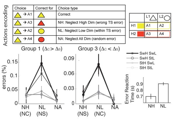
Top-left One-to-one encoding of chosen actions as Correct, NH, NL or NA, as a function of trial input. Top-right Correct actions table for asymptotic learning phase, represented here with color as high dimension context, and shape as low dimension stimulus. Bottom-left, middle proportion of trials as a function of error types, for high and low dimension switch trials (swH and swL) or stay trials (stH and stL), for C-Structure (left) and S-Structure (middle) goups. Bottom-right High dimension switch error reaction-times were faster than those for low dimension switches.

There was a main effect of switch vs stay on the high input dimension H, as expected for an accuracy-based switch-cost (F = 17.65, p < 10⁻³). There was also main effect of error type (F = 27.43, p < 10⁻³), with more NL errors than NH errors (t = 4.57, p < 10⁻⁴) and more NH errors than NA errors (t = 2.21, p = 0.03). Furthermore, these two components to errors (switch vs error type) interacted (F = 11.55, p < 10 − 3): while the effect of errors remained significant both for high dimension switch and stay trials (F = 29.7, p < 10⁻⁴; F = 4.2, p = 0.021 respectively), the increase in errors due to switches on the higher dimension were selectively associated with increased neglect of the lower dimension (t = 5.6, p < 10⁻⁵; other errors p > 0.24). Note that this effect cannot be interpreted as purely driven by attention due to the dimensional switch: such an account would predict a similar effect of switches on the lower dimension leading to neglecting the higher dimension, but this was not observed. Instead, further data (see next paragraph) allow us to understand this result as indicating that subjects correctly update the task-set from one trial to the next based on the higher order dimension, but that they sometimes fail to properly apply it – thus leading to within set errors, rather than perseverative errors. Note that this pattern of errors is predicted correctly by the neural network model. Although it is not directly predicted by the structure model C-TS, it can be accounted for by within-TS noise parameter ∊_TS, as shown earlier in the section linking modeling levels.

Finally, we analyzed reaction times in error trials to provide a clue as to whether higher and lower dimensions might be processed in temporal sequence as predicted by the structured models. We found that on a high dimension switch, NH errors were significantly faster than corresponding NL errors (t = 4.08, p < 10⁻⁴, fig 13). This pattern supports the view that NH errors reflect the impulsive application of the previous trial’s task-set, whereas NL errors occur after the time consuming process of (successful) task-switch. Again, this behavioral result was predicted by the neural network model.

Next, we fit models to subjects behavior to determine whether they are well captured by the C-TS model. Later, we show that the array of qualitative patterns of behavior observed here is robust, by replicating it in a second experiment.

7.4 C-TS Model Fittings

We first focused on comparing the flat model to the two variants of TS-structure model, C-TS(s) and S-TS(c). Model fittings were accomplished by selecting parameters that maximized the likelihood of observed sequence of choices, given the model and past trials. Fits were evaluated using pseudo-r² (assessing the proportion of improvement in likelihood relative to a model predicting chance on all trials; (Camerer & Hua Ho, 1999; Daw & Doya, 2006; Frank et al., 2007a). For models with different numbers of parameters we evaluated fit with Akaike’s Information Criterion (AIC), which penalizes fit for additional model parameters (Burnham & Anderson, 2002; Akaike, 1974). Because alternative models predict nearly identical behavior in initial learning, we restricted the trials considered for the likelihood optimization to the asymptotic learning phase and test phase, without loss of generality.

The flat model included 3 parameters: n₀, the strength of the beta prior p₀ = P(r = 1∣(c, s), a), p₀ ~ Beta(n₀, n₀) played the role of learning speed (since updates to reward expectations are reduced with stronger priors); an inverse temperature softmax parameter (β) and an undirected stimulus-noise parameter ∊. TS-structure models also included 3 parameters: the clustering α parameter, the softmax β parameter and the undirected stimulus-noise parameter ∊. We checked that inclusion of all 3 parameters provided better fit of the data than any combination of 2 of them (fixing the third to canonical values ∊ = 0 or n₀ = 1, and β to the mean fit over the group), again controlling for added model complexity using AIC. For the C-TS model, we also confirmed that inclusion of a supplementary softmax parameter on TS selection did not improve fits and hence use greedy selection of the most likely TS.

Comparing model fit across the 3 models and the 3 groups yielded no main effect of either factor (both F’s < 1.85, p’s > 0.17, ie. there was no overall differences in model fits across the group, or in average fits between groups), but a strong interaction between them (F = 10.6, p < 1.5 10⁻⁶). Post-hoc tests confirmed what is expected from all three groups: indeed, for group 1 and 3, TS-structure models fit significantly better than the flat model (both t’s > 2.2, p = 0.05, fig 6 top), which was not the case for group 2 (t = 0.15, p = 0.88). Furthermore, for group 1, C-TS(s) structure fit significantly better than S-TS(s) structure (t = 2.75, p = 0.02) while the contrary was true for group 3 (t = 4.76, p = 7 10⁻⁴) (see fig 14 top).

Figure 14. Model-fitting.

Top Left: Difference in pseudo-r2 fit value between C-TS(s) vs. S-TS(c) structure model, and overall structure vs. flat models. Group 1 and 3 are better fit by structure than flat, respectively by C and S- TS structure models. Differences in fit values are small because model prediction differences are limited to few trials mostly in the beginning of the test phase. Top Right: Predicted hybrid model probabilities using individual subject-fitted parameters against observed probabilities. Bottom: mean attentional for the 3 experts in competition within a single model confirm results from the separate fits.

The above model fits made a somewhat unrealistic assumption that each group had a learning method fixed at the onset of the experiment, including which input dimension should be used as a context in the structured case. We therefore also considered the possibility that all three options are considered in parallel, in a mixture of three experts, and weighted against each other according to estimated initial priors in favor of each expert and their prediction capacities (cf. Frank & Badre, 2011). This model was presented earlier as the generalized structure mixture model.

Controlling for added model complexity with AIC, we found that this model fit better than any of the three experts embedded within. Mean pseudo-r² was 0.58. We then confirmed previous results by exploring the relative mean fitted weights over the test phase assigned to each expert by each group. Again, we observed no main effects, but a significant interaction between group and expert (F = 3.06, p = 0.023, fig 14 bottom). Interestingly, group 2 subjects had significantly stronger flat expert weights than both other groups (t = 2.24, p = 0.03). Furthermore, within structure weights, the preference for C-TS(s) was significantly stronger for group 1 than for group 3 (t = 2.56, p = 0.019).

Thus, model fitting results confirmed that group 1 and 3 seemed to build TS structure according to Color and Shape respectively. It should be noted that this is not a trivial result: the assignment of subjects to groups was not determined by their performance in the transfer phase, but rather by their reaction time switch-cost during the asymptotic learning phase, to which the model fitting procedure had no access (RTs are not used for fitting). Nevertheless, the results for group 2 remain ambiguous: although it seems that they rely more on flat expert than other two groups, consistent with their low switch-cost on either dimension, the flat model did not fit significantly better than structured models, and structured weights remained significantly positive, as could be expected from the presence of a transfer effect for group 2.

Fitted parameters between groups differed only in the initial priors assigned to each expert. For group 1, the prior for C-TS(s) structure was significantly greater than the other groups (t = 2.7, p = 0.01). Conversely, for group 2, the prior for flat structure was significantly greater than the other groups (t = 2.23, p = 0.03). All other parameters showed no group effects (F’s < 0.84, ns), except for a non-significant trend for parameter ∊ (p = 0.07). Of note, there was no group effect on parameter α (mean α = 4.5; F = 0.57, ns), suggesting that individual differences in transfer were not due to differential tendencies to revisit previous task-sets, but instead seem to reflect differences in the prior tendencies.

7.5 Experiment 2: replication and extension

This replication experiment was similar to that in experiment one, with the following changes.

• Most significantly, given that we had some success in predicting the nature of transfer according to RT switch cost during the learning phase of experiment one, in experiment two we assessed the switch cost during the experiment itself, and used that information to decide which visual input dimension should be considered context. Specifically, if color switch cost was greater than shape switch cost, the test phase inputs corresponded to two new colors and old shapes. This procedure allows us to test whether subjects would generalize their knowledge in the test phase to new contexts regardless of which one they chose to be ‘higher’ dimension during learning, and commits to the switch-cost metric for assessing structure.

• Visual input dimensions were color and shape for all subjects.

• Motor responses were given with four fingers of the main hand.

• We controlled the task sequence in the transfer phase such that the first correct response of the two new contexts associated with stimulus S1 was defined as C3. This allowed us to test transfer without regard for a possible higher level strategy participants could apply. Specifically, some subjects may assume a one-to-one mapping between the 4 possible actions and the 4 different inputs during each experimental phase. This strategy can cause subjects to be less likely to repeat action A1, even though it actually applies to both C3 and C4, which would reduce the likelihood in observing transfer if they happened to respond correctly to C4 first. Of course if analyzed as such there would be a bias favoring transfer because C3-S1 performance is by definition better early during learning than C4-S1. To avoid this bias, we limit all assessment of transfer to the S2 stimuli. Task-set generalization is thus expected to improve performance on S2 for C3 but not C4 without being influenced by S1 stimuli.

• The experiment was repeated three times (with different shapes/colors) for each subject.

7.6 Sample

40 subjects participated in the replication experiment. Technical software problems occurred for two subjects, and three subjects failed to attend to the task (as indicated by a large number of non responses) and were thus excluded from analysis. Final sample size was N=35 subjects.

7.7 Experiment 2 results

First, it should be noted that half of the subjects (N = 18), utilized color as the context dimension as assessed by the switch-cost comparison procedure, while the other half utilized shape, thus confirming our earlier findings that (at least in this experimental protocol) there was no overall bias to treat one dimension or another as context or higher order.

Moreover, this replication experiment confirmed most of the previously described results. Positive transfer, defined as early performance improvement in transfer test condition C3 compared to new test condition C4, was significantly positive (p = 0.036, t = 2.12, restricted to first iteration of the experiment: p = 0.034, t = 2.2). Although the interaction typical of negative transfer is not significant, we get a similar trend: subjects make significantly more NH errors in the C4 condition than in C3 (p = 0.048, t = 2.05), while the difference for NL or NA errors is not significant. This pattern especially holds if restricted to the first iteration of the experiment for each subject (NC p = 0.01 and NS p = 0.4749; interaction p = 0.1).

We also replicate the asymptotic learning phase error effects. In particular, there was a strong main effect of switch H vs stay H on error proportion (t = 6.13,p < 10⁻⁴), consistent with an error switch cost associated to the reaction time switch cost used to define dimension H. While there was also a main effect of switch L (p = 0.005, t = 3), this effect was significantly weaker than the switch H effect (p = 0.025, t = 2.34). Most importantly, the effect of switch vs stay H, but not L, interacts with error type. NL errors are significantly more important than NH errors for switch H (p = 0.0001, t = 4.52), but not for stay H (p = 0.82, difference t = 4.8, p < 10⁻⁴). Conversely, for the low dimension, NL errors are overall more numerous than NH errors, irrespective of switch or stay L (both p’s< 0.01, difference p = 0.74). This is the exact same pattern we obtained in the main experiment. Furthermore, switch H NH errors are significantly faster than switch L NL errors, again replicating main experiment results (first iteration p = 0.0024, all data p = 0.0038).

8 Discussion

In this paper, we have confronted the interaction between learning and cognitive control during task-set creation, clustering and generalization from three complementary angles. First, we developed a new computational model, C-TS, inspired by nonparametric Bayesian methods (approximations to Dirichlet process mixtures allowing simple online and incremental inference). This model specifies how the learner might infer latent structure and decide whether to re-use that structure in new situations (or across different contexts), or to build a new rule. This model leverages structure to improve learning efficiency when multiple arbitrary contexts signal the same latent rule, and also affords transfer even when structure is not immediately evident during learning. Second, we developed a neurobiologically plausible neural network model that learns the same problems in a realistic time frame and exhibits the same qualitative pattern of data indicative of structure building across a wide range of parameter settings, while also making predictions about the dynamics of action selection and hence response times. We linked these neural mechanisms to the higher level computations by showing that the C-TS model mimics the behavior of the neural model and that modulation of distinct mechanisms were related to variations in distinct C-TS model functions. Third, we designed an experimental paradigm to test predictions from both of these models. In particular, we assessed whether human subjects spontaneously build structure into the learning problem when not cued to do so, whether evidence of this structure is predictive of positive and negative transfer in subsequent conditions, and whether the pattern of errors and reaction times are as predicted by model dynamics. We showed across two experiments that the C-TS model provided a good quantitative fit to human subject choices and that dynamics of choice were consistent with the mechanisms proposed.

We thus proposed a new computational model that accounts for the observed behavioral findings. This model learns discrete abstract hidden states that contextualize stimulus-action-feedback contingencies, corresponding to the abstract construct of task-sets. Crucially, task-set representations cannot be substituted with the contexts that predict them (contrary to some models of other tasks, e.g., Frank & Badre (2011)). Rather, the probabilistic link between specific contexts and task-sets is learned over time and used for task-set selection on each trial via a priori inference of the hidden state. This feature is essential for further generalization, since it allows new contexts to potentially be clustered with existing task-sets as diagnostic of a previously learned task-set, rather than automatically assigned to a distinct state. Although this abstract hidden state representation of a task-set feature is present in the model of Collins & Koechlin (2012), that model relied on the assumed episodic stability of external contingencies for task-set inference. Thus to our knowledge the model presented here is the first to allow for simultaneous learning of multiple abstract task-sets in an intermixed procedure that facilitates subsequent generalization.

8.1 Behavioral patterns and model fits indicate incidental structure building

Indeed, the behavioral results robustly indicated that subjects apply cognitive control in a simple learning problem, using one input feature as a higher level context indicative of a task-set, and the other feature as the lower level stimulus. Transfer of these task-sets to new situations led to improved performance when generalization was possible, but also over-generalization and negative transfer in ambiguous new contexts. Moreover, at the individual level, the degree to which these transfer effects were observed was predicted by the nature of the structure built by each subject as inferred by an independent measure (reaction-time switch-costs during the learning phase). This same inferred structure was also predictive of the repartition of error types during both learning and transfer phase, strengthening their validity for identifying the specific hidden structure built by each subject.

In the first experiment, subject groups 1 and 3, who had clearly differentiable switch-costs, showed unambiguous results in favor of the notion that subjects learn hidden structure. Indeed, predictions were confirmed regardless of whether the structure incidentally built turned out to be favorable (group 1), or unfavorable (group 3) to subsequent generalization in the transfer phase of the experiment. Model-fittings also confirmed that subjects from these groups seem to be learning by building hidden task-set structures. However, results for group 2 were more ambiguous, and leave open the question as to whether all subjects tend to infer structure when learning. Indeed, group 2 subjects were identified as those in which we could not detect a reliable difference in reaction-time switch-costs between input dimensions, which is requisite if one serves as higher level context and the other as stimulus. Surprisingly, these subjects nevertheless showed some evidence for positive transfer, and a non-significant but numerical trend towards negative transfer. Two distinct explanations are possible for these seemingly paradoxical results. The first explanation might be that group 2 subjects actually belong to group 1 or 3, but that the RT switch cost measure was not sensitive enough to detect it. This would explain the presence of transfer effects, and would imply that all groups tended to build hidden structure during the learning phase. Alternatively, group 2 subjects might indeed not have built any structure during the learning phase, instead learning in a flat way, as suggested by switch cost and model-fitting results. However, to account for observed transfer effects, we would then have to suppose that during the test phase, subjects build a posteriori structure retrospectively, performing backwards inference and reorganizing learning phase observations as a consequence of test phase observations (evidence for backward inference, although on simpler schemes, is abundant even in infants; Sobel & Kirkham (2007)). Relatedly, it is possible that these subjects kept track of different possible structures during learning, including both flat and structured experts and then adjusted their attentional weights toward structured expert during transfer when the evidence supported C-TS structure over the others, as was the case in the generalized structure model presented above. These different possibilities cannot easily be discriminated based on the current findings, but may be addressed in future research.

Group 2 findings notwithstanding, we showed that most subjects tend to build hidden structure in a simple learning paradigm that does not require or even benefit from it during acquisition. We replicated this finding in a second experiment in which, by design, all subjects were in group 1 or 2 (that is, they were all afforded the potential to transfer task-set knowledge defined by the structure they most likely built). We emphasize again that when viewed only from the perspective of the acquisition phase in this particular task, the tendency to create structure does not seem optimal, in terms of quantity of information to be stored and complexity of the model needed to represent structure. Regarding quantity, building task-sets requires formation of six links (two context-task-sets links, two stimulus-action links per task-set), while learning in a flat way requires only four (one per input). As for the complexity, building structure complicates the credit assignment problem: it requires the agent to disambiguate the hidden state associations and involves wasting some information when an event is assigned to the incorrect hidden state. Indeed, structured models show slightly less efficient initial learning compared to flat models in this task (in contrast to the other task in which there is a benefit to initial clustering). This was especially evident in the neural network, in which we found that the flat single loop neural model acquired the learning contingencies more rapidly than the structured two loop model (but the latter model showed more similar learning speeds to human subjects). The important question thus remains: why do subjects recruit cognitive control to structure learning in simple reinforcement learning problems even if they don’t afford an obvious advantage, and even comes with a computational cost? We propose several directions for this question.

One possibility is that building structure, while apparently unnecessary during learning, may provide an advantage for potential subsequent generalization (despite the fact that subjects were not aware of the ensuing transfer phase). If the potential to generalize learned structure is common in the environment, it might be optimal in the long run to attempt to build structure when learning new problems. Such an incidental strategy for building structure during learning may have therefore developed throughout learning or even evolution in terms of the architecture of cognitive action planning. Indeed, recent neuroimaging and model-fitting experiments suggested that subjects’ tendency to apply hierarchical structure in a task in which there was an advantage to doing so was related to greater activations in more anterior fronto-striatal loops at the outset of the task – as if they search for structure by default (Badre et al., 2010; Badre & Frank, 2011). Indeed, rather than showing increases in such activations with learning, these studies revealed that subjects learned not to engage this system in conditions where it was detrimental to do so, as evidenced by declining activation as a function of negative reward prediction errors (Badre & Frank, 2011). At the behavioral level, this is the same line of argument as proposed by Yu & Cohen (2009) for subjects’ “magical thinking”, or inference of sequential structures in random binary sequences (see also Gaissmaier & Schooler (2008) who demonstrated that seemingly suboptimal probability matching is related to the tendency to search for patterns). This interpretation raises the question of whether structure building is unique to humans or primates, and/or whether deficiencies in the associated mechanisms may relate to developmental learning disabilities involving poor generalization, such as autism (Stokes, 1977; Solomon et al., 2011).

A second possible explanation resides in the nature of input representations. Indeed, when we have described the flat ideal learner we have assumed perfect pattern separation of the four inputs into four states. Because each of these inputs constitutes overlapping two-dimensional images, there may be some interference between them at either perceptual or working memory stages (e.g., proactive interference; Jonides & Nee (2006)). In our task, recalling the actions that have been selected for a given colored shape could be rendered more difficult by the presentation of other intervening and conflicting colored shapes. Thus, learning in a flat way would incur a cost to resolving the interference between the input representations. That cost may be absent in the structured representations: depending on the task-set selected, the same stimulus may be assigned a distinct representation. Thus, learning structure might be helpful in separating conflicting representations of the task, apart from its potential advantage in further generalization.

A third possible explanation for why subjects create structure is that learning in a flat way requires identifying which of the four inputs and which of the four actions is currently relevant. Learning in a structured way, however, cuts these four-way decisions into two successive two-way decisions: first identifying which of the two contexts and hence which task-set is applicable, then which of the two stimuli and hence which action is appropriate. Learning in a hierarchical structure might then be seen as a way to transform one difficult decision problem into two simpler sequential decisions, or “divide and conquer” strategy. This issue is of particular interest in light of the debate on the functional organization of prefrontal cortex, which is crucially involved in cognitive control and task-set selection, with more posterior premotor areas involved in simple stimulus-action selection. Indeed, the rostro-caudal axis has been known to encode a gradient of representations for cognitive control, with the nature of this gradient being at the heart of the debate. There have been arguments for a pure level of policy abstractness gradient (Badre, 2008), for a pure temporal gradient (Fuster, 2001), or for a mixture of both (Koechlin et al., 2003). While task-set selection may typically be considered structure abstraction, in our models it also involves a sequential decision making process and thus also involves a temporal gradient.

Our data provide one argument in favor of this sequential interpretation. When task-switching fails, the nature of errors depended on the speed with which subjects (and networks) responded, with the pattern implying an initial time-consuming task-set selection process followed by action selection within the task-set. Specifically, fast errors corresponded to an impulsive re-application of the previously selected (but now incorrect) task-set. In contrast, slow errors reflected correct task-set updating but then a mis-identification of the lower level stimulus. Note that the vast majority of the task-switching literature has made it impossible to separate these types of errors, due to the use of two-response tasks (so that an error always corresponds to a single response). The error switch-cost has been mostly attributed to two mechanisms: the persistence of the previous task-set, and the reconfiguration of the new task-set (Monsell, 2003; Sakai, 2008). We show here that errors following task-set switches more often result from inappropriate application of the task-set to the current stimulus than to perseveration of the previous trial’s task-set. ¹⁴

8.2 Model sub-optimality and limitations

Although the C-TS model is inspired by the optimal non-parametric Bayesian approach (specifically, Dirichlet process mixtures), we do not claim that optimal computation of the defined probabilistic model of the environment. Indeed, the model includes several non-Bayesian approximations, which also makes it more similar to the neural implementation. The main approximation consists of a discrete and definitive inference of the hidden state, by taking the mode of the distribution (as has been done in similar clustering models of category learning, (e.g. Anderson, 1991; Sanborn et al., 2006)). We adopted this approach both a priori for selecting a task-set (and hence an action selection strategy), and a posteriori for using feedback information to update structure-dependent stimulus-action contingencies. More exact inference requires keeping track of the probability distribution over the partitions of contexts into hidden states, and the hyperparameters defining structure-dependent stimulus-action-outcome probabilities. This highly complex inference is computationally very costly. We found that our simple approximation resulted in the same overall qualitative pattern of predictions as the more exact version, and is largely sufficient to afford computational advantage in learning efficiency when multiple contexts signify the same task-set (though it would possibly fail in much more complex situations). One limitation of the approximation is the inability to retrospectively go backwards in time and reassign a particular trial to a different hidden state when subsequent experiences indicate this should be the case (as is one hypothesis for group 2), as might be done – in a probabilistic sense – by exact inference.

Another limitation in the model is in the absence of sequential structure. We make two assumptions of temporal nature. First, on a large scale, we assume a stable environment with non-varying associations between contexts and task-sets. This assumption can be seen as a first-order approximation, and more work is required to deal with non-stationary relation between contexts and task-sets. Second, on a smaller time scale, we assume no trial-to-trial dependence on action selection (so that the model, in this form, cannot account for working memory tasks such as 12AX O’Reilly (2006), for example). Indeed, while the selection of task-sets on each trial is dependent on its learned value, it is independent of the identity of the previous trial’s context or inferred task-set (unlike the neural model which has persistent activation states making previous trial task-sets more efficiently re-used on the current trial and hence accounting for RT effects). Certainly one could modify the C-TS model specification to accommodate this probability, but that would require also confronting the normative reasons for doing so, of which there are several possibilities that are beyond the scope of this paper.

8.3 Neural network and relationship between levels of modeling

We related the algorithmic modeling level to mechanisms embedded within a biologically inspired neural network model. Although (as we discuss at the end of this section) there are some differences between the core computations afforded by the two levels of modeling, at this stage we have focused on the complementary ways of accomplishing similar goals and consider them largely two levels of description that both account for our novel experimental data, rather than as competing models.

The neural network structure relies on the well studied cortico-basal ganglia loops that implement gating mechanisms and unsupervised dopamine-driven reinforcement learning. The network’s functional structure accords with recent evidence showing that the basal ganglia play a crucial role not only in reinforcement learning, but also in modulating prefrontal activity in various high level executive functions, including task-switching (van Schouwenburg et al., 2010; Moustafa et al., 2008) and working memory (O’Reilly & Frank, 2006; Cools et al., 2007; Baier et al., 2010). Similarly to Frank & Badre (2011), and in accordance with the functional organization of corticostriatal circuits, we embedded the learning/gating architecture into two nested loops, with the input of the second loop (both striatum and STN) constrained by the output of the first. However, the specific contribution of the model is in the nature of representations learned. Indeed, the prefrontal loop learns to gate an abstract, latent representation, that only carries “meaning” in the way it influences the second, premotor loop – via the parietal cortex – for the selection of actions in response to stimuli. This function generalizes that in the Rougier et al. (2005) model, which showed how PFC units can come to represent a particular abstract construct (e.g., color rule units) through learning and development. In that case, color rule neurons supported the selection of actions pertaining to specific colors according to task demands. In the current network, PFC units came to represent an entire task-set policy in a hierarchical fashion, dictating how actions should be selected in response to other stimulus dimensions. Also, unlike the Rougier model, our network does not require repeated presentation of the same task rule in blocks of trials for latent representations to develop. The network only created these representations as needed, thus inferring not only the identity of the current hidden task-set, but also the unknown quantity of possible task-sets, and assignment of specific contexts to those relevant task-sets. When new contexts are presented, the network can gate an existing task-set representation which is then reinforced if it is valid. Thus the task-sets are context-independent as found in the literature (Reverberi et al., 2011; Woolgar et al., 2011). Moreover, unlike previous BG-PFC gating models (O’Reilly & Frank, 2006; Frank & Badre, 2011; Reynolds & O’Reilly, 2009; Rougier et al., 2005) which relied on reinforcement learning for gating PFC representations but supervised learning at the level of motor responses, the current model relied on reinforcement learning at all levels (after all, there is no overt supervised feedback in the experiments), making it more challenging. Nevertheless, networks learned in similar number of training experiences as did human subjects. Finally, the quantitative fits of the C-TS model to the BG-PFC networks confirmed that the gating of distinct PFC states corresponded well to the creation, clustering and re-use of task-sets.

The current model relies crucially on diagonal projections across loops¹⁵ While large-scale cortico-basal ganglia loops were originally characterized as parallel and segregated, there is now ample evidence of integration between circuits (Haber, 2003). Here, we included a projection from anterior frontal regions to the motor STN and motor striatum (Nambu, 2011; Haber, 2003). The diagonal STN projection plays a important role in regulating gating dynamics to ensure that motor action selection is prevented until the appropriate task-set is selected. While this slows responding somewhat, it parametrically improves learning efficiency by reducing interference, and (unlike the algorithmic model) naturally accounted for the pattern of RTs across different error types. Variations in this projection strength were captured in the C-TS model fits by a parameter affecting noise in task-set selection in response to contexts. In contrast, the diagonal striatum projection facilitates preparation of actions concordant with the selected task-set independent of the stimulus, and accounts for the greater proportion of within task-set (NL or NS) than across task-set (NH or NC) errors during learning. Accordingly, variations in this projection strength was captured in the C-TS model fits by a parameter affecting within task-set noise.

Overall, we showed that the full pattern of effects exhibited by subjects and captured by this model were robust to wide range of variations in key parameters (figure 7).

The different levels of modeling bring different ways of understanding human behavior and neural mechanisms thereof. On one hand, the computational C-TS model affords quantitative predictions and fits to subject behavior from a principled perspective. On the other hand, the neural network, aside from its clear links to neuroscience data, naturally captures within-trial dynamics, including reaction times, as well as qualitative predictions on larger time scale dynamics. We showed that the clustering of contexts onto PFC states in the neural model was related to benefit in initial learning when task structure was present, and to generalization during transfer. Quantitative fits showed that the behavior of the more complex neural model was well captured by the C-TS model (see also Frank & Badre (2011); Ratcliff & Frank (2012) for similar approaches), with roughly the same fit as that to human subject choices. Moreover, the latent variables inferred by C-TS corresponded well to the PFC state selected by the neural network, and the effects of biological manipulations were captured by variations in distinct parameters within the C-TS framework. For example, parametric manipulations of the prior tendency to represent distinct contexts as distinct PFC states were directly related to the fitted α parameter, suggesting that this tendency can be understood in terms of visiting new states in a Dirichlet process mixture. In this task context, thus, the nested gating neural network might be understood as implementing an approximate inference in a Dirichlet process mixture.

However, although the neural model was well fitted by the C-TS model across multiple tasks and manipulations, there remain some significant functional differences. Most notably, the C-TS model is able to infer a posteriori the nature of the hidden state regardless of the state that it selected for that trial a priori (by computing likelihoods given both selected and non selected task-sets), and uses that inference to guide learning. In contrast, the neural network only learns the value of the PFC task-sets (and motor actions) that have been gated in each trial, and does not learn about unselected task-sets. To examine this difference more carefully, we conducted an auxiliary simulation in which the C-TS model mimicked this more restricted network capacity, so that there was only a posteriori updating of the a priori selected task-set and action. This simulation produced only slightly less efficient behavior, and provided very similar fitting results to human subjects’ behavior. This result suggests that human learning is well captured by approximations to Bayesian computations consistent with the implementation in our neural network. However, it is entirely possible that our task paradigm was not sensitive enough to differences in the two forms of learning and other paradigms may show that human learning and inference capacities may exceed that of the neural network. Another difference resides in the specific prior for clustering contexts within task-sets, which we implemented in the simplest way possible in the network, since it was not critical for the simulated experiments. An interesting avenue for further experimental and modeling research is to test whether subjects indeed rely on the assumed Dirichlet process prior for building task-sets (i.e., do they attempt to re-use them in proportion to their popularity across multiple contexts). Such a finding would motivate the use of simple mechanisms to build this prior into the neural network.

Finally, the neural model also allows us to make specific predictions for future experiments with neurological populations, pharmacological manipulations, and neuroimaging. For example, probabilistic tractography can be used to assess whether projections from PFC to STN are predictive of individual differences in the RT differences between NH and NL errors, as predicted by our model.

8.4 Relationship to hierarchical reinforcement learning

The models can be seen as a hierarchical model for learning cognitive control structure. Indeed, stimulus-action selection at the lower level is constrained by its parallel higher level context-task-set selection. Apart from the models already discussed, specifically aimed at learning task-set hierarchy, other models have focused on hierarchical reinforcement learning (Botvinick, 2008). This framework augments standard RL by allowing the agent to select not only “primitive” motor actions, but also higher level “options” that constrain primitive action selection (in the same way that task-sets do). However, the crucial distinction between this hierarchical framework and the one we propose here relies in the nature of the hierarchy considered. Indeed the options framework builds a sequential hierarchy: it transforms a Markov decision process into a semi-Markov decision process, by allowing entire sequences of actions to be selected as an option. The hierarchy here thus lies in the temporal sequencing and resolution of the decision process. In our case however, the hierarchical structure is present within each trial and does not affect sequential strategy (see also Frank & Badre (2011) for more discussion on the potential overlap with the options framework at the mechanism level). Thus, these models address different aspects of hierarchical cognitive control. Nevertheless, if we extend our TS paradigms to situations in which the agent’s action affects not only the outcome but the subsequent state (i.e. the transition functions are non-random), then the selection of a TS is similar to the selection of an option policy. Indeed, in preliminary simulations not presented here, we found that the C-TS model provides a similar advantage to the options framework in learning extended tasks with multiple sub-goals needed to reach an end goal (the “rooms” grid-world problem discussed in Botvinick (2008)) ¹⁶. In contrast, the options framework does not consider structure in the state space for determining which policy applies (it focuses on structure within hierarchical sets of actions). Thus, it has no mechanism to allow clustering contexts indicative of the same option – its ability to generalize options applied toward larger goals relies on observing the identical states in the subgoals as observed previously.

8.5 Relationship to category learning

As noted in the introduction, our approach also borrows from clustering models in the category learning literature (Anderson, 1991; Sanborn et al., 2006). Whereas category learning typically focuses on clustering of perceptual features onto distinct categories, our model clusters together contextual features indicative of the same latent more abstract TS. Thus the clustering problem allows identification of the correct policy of action selection given states, where the appropriate policies are likely to be applicable across multiple contexts.

Note that the similarity between different contexts can only be observed in terms of the way the set of stimulus-action-outcome contingencies, as a group, are conditioned by these contexts. Thus, whereas in category learning experiments a category exemplar is present on each trial, in the TS situation only one ‘dimension’ of a latent TS is observed on any one trial (i.e. only one of the relevant stimuli is presented, and only one action selected). Thus whereas category learning models address how perceptual features may be clustered together to form a category rule, potentially even inferring simultaneously different relevant structures as we do (Shafto et al., 2011), here we address how higher level contextual features can be clustered together in terms of their similarities in identifying the applicable rule. Furthermore, unlike in perceptual category learning, the identity of the appropriate task-set is never directly observable by subjects through feedback: feedback only directly reinforces the appropriate action, not the overarching task-set. For the same reasons, subjects’ beliefs about which task-set applies are not directly observable to experimenters (or models).

Other category learning models focus on the division of labor between BG and PFC in incremental procedural learning vs rule-based learning, but do not consider rule clustering. In particular, the COVIS model (Ashby et al. (1998)) involves a PFC component that learns simple rules based on hypothesis testing. However, COVIS rules are based on perceptual similarity, and focus on generalization across stimuli within rules, rather than generalization of rules across unrelated contexts. Thus although COVIS could learn to solve the tasks we study (in particular, the flat model is like a conjunctive rule), it would not predict transfer of the type we observe here to other contexts. Other models rely on different systems (such as exemplar, within category clusters, and attentional learning) to allow learning of rules less dependent on similarity (Kruschke, 2011; Love et al., 2004; Hahn et al., 2010). Again, these models do not allow generalization of rules across different contexts, but only potentially across new stimuli within the rules.

8.6 Conclusion

Cognitive control and learning behavior are mostly studied separately. However, it has long been known that they implicate common neural correlates, including prefrontal cortex and basal ganglia. Furthermore, they are strongly intermixed in most situations: learning, in addition to slow error driven mechanisms, implicates executive functions in a number of ways, including working memory, strategic decisions, exploration, hypotheses testing, etc. Reciprocally, cognitive control relies on abstract representations of tasks or rules, that often take a hierarchical structure (Badre, 2008; Botvinick, 2008; Koechlin & Summerfield, 2007) that need to be learned. It is thus crucial to study both simultaneously. We have proposed a computational and experimental framework that allowed us to make strong predictions on how cognitive control and learning interact. Results confirm model predictions, and show that subjects have a strong tendency to apply more cognitive control than immediately necessary in a learning problem: subjects build abstract representations of task-sets preemptively, and are then able to identify new contexts to which they can generalize them. This tendency to organize the world affords advantages when the environment is organized, but potential disadvantage when it is ambiguously structured. We explored a potential brain implementation of this interaction between cognitive control and learning, with predictions to be investigated in future research.

Figure 15. Generalized structure model.

In the above depiction we considered models for representing different sorts of structure, C-TS, S-TS, or flat. The generalized structure model represents all of these as potential descriptors of the data, and infers which one is more valid. We considered two ways to approach this issue: the first uses a mixture of experts architecture in which each expert learns assuming a different sort of structure, and then weights them according to their inferred validity for action selection. The second strategy considers all of the potential structures within the generative model itself. Both models produced similar behavior and predictions.

Appendix

9 Appendix: Algorithmic models details

9.1 C-TS model details

For all TS_i in the current TS space {1, … , n_TS(t)}, and all contexts c_j experienced up to time t, we keep track of the probability that this task-set is valid given the context p(TS_i∣c_j), implicitly conditionalized on past trial history. The most probable task-set TS_t in context c_t at trial t is then used for action selection: TS_t = argmax_i=1…nTS(t) P(TS_i∣c_t).

Specifically, action selection is determined as a function of the expected reward values of each stimulus action pair given the selected task-set TS_t, Q(s_t, a_k) = E(r∣s_t, a_k, TS_t). The policy function as a function of Q can be a softmax action choice (see equation 4), but is detailed in the section 9.4.

Belief in the applicability of all latent task-sets is updated after observation of reward outcome r_t. Specifically, the estimated posteriors for all TS_i ∈ [i = 1 … n_TS(t)] are updated to:

$$P_{t+1}({\mathit{TS}}_i\mid c_t)=\frac{P(r_t\mid s_t,a_t,{\mathit{TS}}_i)\times P({\mathit{TS}}_i\mid c_t)}{\sum _{j=1\dots N_{\mathit{TS}}\left(t\right)}P(r_t\mid s_t,a_t,{\mathit{TS}}_j)\times P({\mathit{TS}}_j\mid c_t)]},$$ (5)

where N_TS(t) is the number of task-sets created by the model up to time t (see details below). We then determine, a posteriori, the most likely task-set associated to this trial: TS’_t = argmax_i=1…nLS(t) P_t+1(TS_i∣c_t). This determines the single task-set for which state-action learning occurs in this trial ¹⁷ : P(r∣s_t, a_t, TS’_t) ~ Bernoulli(θ), θ ~ Beta(n₀+n_t+1(TS’_t, s_t, a_t), m0+m_t+1(TS’_t, s_t, a_t)), where (n₀, m₀) correspond to the prior initialization on the task-set’s Bernoulli parameter, and (n_t, m_t) are numbers successes (r = 1) and failures (r = 0) observed before time t for (TS’_t, s_t, a_t), such that we increment n_t+1(TS’_t, s_t, a_t) = n_t(TS’_t, s_t, a_t) + r_t, and m_t+1(TS’_t, s_t, a_t) = m_t + (1 − r_t).

For each new (first encounter) context c_n+1, we increase the current space of possible hidden TS by adding a new TS_new to that space. This task-set is blank in that it is initialized with prior belief outcome probabilities P(r∣s_i, a_i) ~ Bernoulli(θ), θ ~ Beta(n₀, m₀), with n₀ = m₀. We then initialize the prior probability that this new context is indicative of TS_new or whether it should instead be clustered to any existing TS, as follows.

$$P({\mathit{TS}}^{\ast }=.\mid c_{n+1})=\{\begin{array}{ccc}\hfill P({\mathit{TS}}^{\ast }={\mathit{TS}}_{\mathit{new}}\mid c_{n+1})& \hfill =\hfill & \alpha ∕A\hfill \\ \hfill \forall i\ne \mathit{new},P({\mathit{TS}}^{\ast }={\mathit{TS}}_i\mid c_{n+1})& \hfill =\hfill & \sum _{j}P({\mathit{TS}}_i\mid c_j)∕A\hfill \end{array}\phantom{\}}$$ (6)

Here, α determines the likelihood of visiting a new TS state (as in a Dirichlet / Chinese restaurant process), and A is a normalizing factor: A = α + ∑_i,j P(TS_i∣c_j).

9.2 Flat model

The most common instantiation of a flat model is the delta learning rule (equivalent to Q-learning in a first order Markovian environment). Here, the “state” comprises the conjunction of stimulus and context (e.g., shape and color), and the expected value of each state-action pair is updated separately in proportion to reward prediction error:

$$Q\left(\right(c_t,s_t),a_t)=Q\left(\right(c_t,s_t),a_t)+\text{learning rate}\times [r_t-Q((c_t,s_t),a_t\left)\right].$$ (7)

For coherence when comparing with more complex models, we instead implement a Bayesian version of a flat learning model: for each input-action pair, we model the probability of a reward as a belief distribution P(r_t∣(c_t, s_t), a_t) ~ Bernoulli(θ), with prior θ ~ Beta(n₀+n_t, m₀+m_t). Each positive or negative outcome is treated as an observation, allowing straightforward Bayesian inference on the beta distribution, with n_t and m_t indicating the number of positive and negative outcomes observed up to trial t, and n₀ and m₀ defining the prior.

Policy is determined by the commonly used softmax rule for action selection as a function of the expected reward for each action, as defined in equation 4 in main text.

9.3 Generalized structure model

The mixture of experts includes a C-TS(c) expert, a S-TS(c) expert and a flat expert (similar to Frank & Badre, 2011). All experts individually learn and define policies as specified previously. Learning and choice contributions are weighted in proportion to expert reliability, as follows:

$$p\left(a\right)=w_{\mathit{flat}}\times p_{\mathit{flat}}\left(a\right)+w_{C-\mathit{TS}\left(s\right)}\times p_{C-\mathit{TS}\left(s\right)}\left(a\right)+w_{S_{T}S\left(c\right)}\times p_S\left(a\right),$$ (8)

where weights reflect the probability that each expert is valid, as inferred using learned likelihoods of observed outcome after each trial (learning for each expert is similarly weighted by their reliability). For example, w_C−TS(s)(t + 1) ∝ w_C−TS(s)(t) × P(r_t∣s_t, a_t, TS_t). Weights were initialized with initial estimated parameters with constraint that they sum to 1, so that w_flat(0) = w_F, w_C−TS(s)(0) = (1 − w_F) × w_C, and w_S−TS(c)(0) = (1 − w_F) (1 − w_C). We also allowed for forgetting in the update of weights to make them tend to drift towards initial prior (allowing for the possibility that the correct expert describing the task structure may have changed) so that at each trial,

$$w_{\text{expert}}\left(t\right)=\tau \times w_{\text{expert}}\left(t\right)+(1-\tau )\times w_{\text{expert}}\left(0\right).$$ (9)

Finally, for model-fitting purposes we assumed the possibility of differential learning speed between flat and TS-expert models, given that the flat (conjunctive) expert includes more individual states (Collins & Frank, 2012).

To implement the generalized structure within the generative model itself, we mixed predicted outcomes from each potential structure into a single policy, rather than mixing policies from distinct experts. This model considers the predicted outcome given each of the potential structures, P(r∣a, I), where information I indicates stimulus and most likely task-set for each of the structures, or the (C,S) conjunctive pair for the flat model. In this formulation, a global expected outcome is predicted by mixing these expected outcomes according to uncertainty w in the validity of which structure applies. A single softmax policy is then used for action selection based on this integrated expected outcome. This version is a different approximation to the mixture of experts implementation, but both lead to very similar behavior in simulations. We give an example simulation in figure 16.

9.4 Noise and interindividual variations

To account for suboptimal behavior and individual differences when we fit this model to human and neural network models, we allow for 3 natural levels of noisy behavior. Recall that in the model described above, the most likely task-set was always selected prior to action selection. We replace this greedy task-set selection with a softmax choice rule, with parameter β_TS: the probability of selecting TS_i is

$$\pi \left({\mathit{TS}}_i\right)=\frac{{\beta }_{\mathit{TS}}P({\mathit{TS}}_i\mid c_t)}{\sum _{j=1\dots n_{\mathit{TS}}}{\beta }_{\mathit{TS}}P({\mathit{TS}}_j\mid c_t)}.$$

Learning about the task-sets is then also weighed by their likelihood.

Given the selected task set, we include noisy/exploration processes on action selection. In addition to the usual action exploration through softmax as a function of Q(s, a_k) = E(r∣s_t, a_k, TS_t) we also allow for noise in the recognition of the stimulus on which the task-set is applied:

$$p(a_k\mid s_t,{\mathit{TS}}_t)=∊\times \mathit{softmax}(a_k\mid {\mathit{TS}}_t,s\ne s_t)+(1-∊)\times \mathit{softmax}(a_k\mid {\mathit{TS}}_t,s_t),$$ (10)

where ∊ estimates noise in stimulus classification within a task-set (or noise in task-set execution), and allows for a small percentage of trials in which the stimulus is misidentified while the task-set is selected appropriately.

Finally, we parameterize the strength of initial priors on the new task-sets’ Bernoulli parameter, by setting them to Beta(n₀, n₀). A non-informative prior would be set with n₀ = 1, but we allow n₀ to vary, thus effectively influencing the learning rate for early observations. It is reported as i₀ = 1/n₀, to be positively correlated with a learning speed.

9.5 Flat model variant: Mixture of dimension experts

In this model, we allow for the specific nature of input states to be taken into account, namely their representation as two-dimensional variables. Action selection results from a mixture of three flat “experts” (fig 11c): a conjunctive (C-S)-expert, identical to the previously described flat model, a C-expert and an S-expert. Both single dimensional experts are identical to the full flat expert, except that the input state (c_t, s_t) is replaced by the appropriate single dimensional input c_t or s_t respectively. Action selection is determined by a weighted mixture of the softmax probabilities (equation 4) defined by all three experts:

$$p\left(a\right)=w_{\mathit{flat}}\times p_{\mathit{flat}}\left(a\right)+w_C\times p_C\left(a\right)+w_S\times p_S\left(a\right).$$ (11)

Weights reflect the estimated probability of each expert being valid, inferred using learned outcome likelihoods: for example, w_C(t + 1) ∝ w_C(t) × P(r_t∣c_t, a_t).

Depending on the parameters chosen, this model is also able to learn near optimally during the initial phase. During the transfer phase, the S-expert should initially predict outcomes better than the full flat expert, because valid actions are taken from the actions previously valid for similar shapes (ie., visuomotor bias). It thus predicts that the S-expert should contribute more to action selection in the test phase. Since that advantage is identical in both C3 and C4 conditions, the model predicts no difference in learning curve between them(fig 11d). However, the preponderant role of the S-expert can be observed in that more errors corresponding to the S-correct actions for the other color are committed than other errors. Specifically, this model predicts more NC errors (neglect color) than NS or NA errors for both C3 and C4 (fig 11g inset).

10 Appendix: Neural model implementational details

The model is implemented using the emergent neural simulation software (Aisa et al., 2008), adapted to simulate the anatomical projections and physiological properties of BG circuitry in reinforcement learning and decision making (Frank, 2005, 2006). Emergent uses point neurons with excitatory, inhibitory, and leak conductances contributing to an integrated membrane potential, which is then thresholded and transformed to produce a rate code output communicated to other units. There is no supervised learning signal; reinforcement learning in the model relies on modification of corticostriatal synaptic strengths. Dopamine in the BG modifies activity in Go and NoGo units in the striatum, where this modulation of activity affects both the propensity for overall gating (Go relative to NoGo activity), and activity-dependent plasticity that occurs during reward prediction errors (Frank, 2005; Wiecki et al., 2009). Both of these functions are detailed below.

The membrane potential V_m is updated as a function of ionic conductances g with reversal (driving) potentials E according to the following differential equation:

$$\begin{array}{cc}\hfill C_m\frac{{\mathit{dV}}_m}{\mathit{dt}}=& g_e\left(t\right){\stackrel{‒}{g}}_e(E_e-V_m)+\hfill \\ \hfill & g_i\left(t\right){\stackrel{‒}{g}}_i(E_i-V_m)+\hfill \\ \hfill & g_l\left(t\right){\stackrel{‒}{g}}_l(E_l-V_m)+\hfill \\ \hfill & g_a\left(t\right){\stackrel{‒}{g}}_a(E_a-V_m)+\hfill \\ \hfill & \dots ,\hfill \end{array}$$ (12)

where C_m is the membrane capacitance and determines the time constant with which the voltage can change, and subscripts e, l, i and a refer to excitatory, leak, inhibitory and accommodation channels respectively (and “..” refers to the possibility of adding other channels implementing neural hysteresis). The reversal or equilibrium potentials E_c determine the driving force of each of the channels, whereby E_e is greater than the resting potential and E_l and E_i are typically less than resting potential (with the exception of tonically active neurons in GPi and GPe, where leak drives current into the neuron; Frank (2006)). Following electrophysiological convention, the overall conductance for each channel c is decomposed into a time-varying component g_c(t) computed as a function of the dynamic state of the network, and a constant $\overline{g_c}$ that controls the relative influence of the different conductances. The excitatory net input/conductance g_e(t) is computed as the proportion of open excitatory channels as a function of sending activations times the weight values:

$$g_e\left(t\right)=\langle x_i{w}_{\mathit{ij}}\rangle =\frac{1}{n}\sum _i{x}_i{w}_{\mathit{ij}}$$ (13)

For units with inhibitory inputs from other layers (red projections in Figure 4), predominant in the basal ganglia, the inhibitory conductance is computed similarly, whereby g_i(t) varies as a function of the sum of the synaptic inputs. Dopamine also adds an inhibitory current to the NoGo units, simulating effects of D2 receptors. (See below for a simplified implementation of within-layer lateral inhibition). Leak is a constant.

Activation communicated to other cells (y_j) is a thresholded (Θ) sigmoidal function of the membrane potential with gain parameter γ:

$$y_j\left(t\right)=\frac{1}{\left(1+\frac{1}{\gamma {\left[V_m\right(t)-\Theta ]}_{+}}\right)}$$ (14)

where [x]₊ is a threshold function that returns 0 if x < 0 and x if X > 0. (Note that if it returns 0, we assume y_j(t) = 0, to avoid dividing by 0). As it is, this function has a very sharp threshold, which does not fit real spike rates. To produce a less discontinuous deterministic function with a softer threshold, more like that produced by spiking neurons, the function is convolved with a Gaussian noise kernel (μ = 0, σ = .005), which reflects the intrinsic processing noise of biological neurons:

$$y_j^{\ast }\left(x\right)={\int }_{-\infty }^{\infty }\frac{1}{\sqrt{2\pi }\sigma }{e}^{-z^2∕\left(2{\sigma }^2\right)}{y}_j(z-x)\mathit{dz}$$ (15)

where x represents the [V_m(t) − Θ]₊ value, and $x_j^{\ast }\left(x\right)$ is the noise-convolved activation for that value.

10.1 Inhibition Within Layers

For within layer lateral inhibition, Leabra uses a kWTA (k-Winners-Take-All) function to achieve inhibitory competition among units within each layer (area). The kWTA function computes a uniform level of inhibitory current for all units in the layer, such that the k+1th most excited unit within a layer is generally below its firing threshold, while the kth is typically above threshold. Activation dynamics similar to those produced by the kWTA function have been shown to result from simulated inhibitory interneurons that project both feedforward and feedback inhibition (O’Reilly & Munakata, 2000), and indeed other versions of the BG model use explicit populations of striatal inhibitory interneurons, in addition to inhibitory projections from striatum to GPi/GPe, etc (e.g., Wiecki et al., 2009). Thus, the kWTA function provides a computationally effective and efficient approximation to biologically plausible inhibitory dynamics.

kWTA is computed via a uniform level of inhibitory current for all units in the layer as follows:

$$g_i=g_{k+1}^{\Theta }+q(g_k^{\Theta }-g_{k+1}^{\Theta })$$ (16)

where 0 < q < 1 (.25 default used here) is a parameter for setting the inhibition between the upper bound of $g_k^{ϴ}$ and the lower bound of $g_{k+1}^{ϴ}$. These boundary inhibition values are computed as a function of the level of inhibition necessary to keep a unit right at threshold:

$$g_i^{\Theta }=\frac{g_e^{\ast }{\stackrel{‒}{g}}_e(E_e-\Theta )+g_l{\stackrel{‒}{g}}_l(E_l-\Theta )}{\Theta -E_i}$$ (17)

where $g_e^{\ast }$ is the excitatory net input.

Two versions of kWTA functions are typically used. In the kWTA function used in the Striatum, $g_k^{ϴ}$ and $g_{k+1}^{ϴ}$ are set to the threshold inhibition value for the kth and k + 1th most excited units, respectively. Thus, the inhibition is placed to allow k units to be above threshold, and the remainder below threshold.

Cortical layers use the average-based kWTA version, where $g_k^{ϴ}$ is the average $g_i^{ϴ}$ value for the top k most excited units, and $g_{k+1}^{ϴ}$ is the average of $g_i^{ϴ}$ for the remaining n − k units. This version allows for more flexibility in the actual number of units active depending on the nature of the activation distribution in the layer and the value of the q parameter (which is set to default value of .6). This flexibility is generally used for units to have differential levels of activity during settling.

10.2 Connectivity

The connectivity of the BG network is critical, and is thus summarized here (see Frank, 2006 for details and references). Unless stated otherwise, projections are fully connected (that is all units from the source region target the destination region, with a randomly initialized synaptic weight matrix). However the units in PFC, PMC, Striatum, GPi/GPe, Thalamus and STN are all organized with columnar structure. Units in the first stripe of PFC/PMC represent one abstract task-set/motor action and project to a single column of each of Go and NoGo units in their corresponding Striatum layer, which in turn projects to the corresponding columns in GPi/GPe and Thalamus. Each Thalamic unit is reciprocally connected with the associated column in PFC/PMC. This connectivity is similar to that described by anatomical studies, in which the same cortical region that projects to the striatum is modulated by the output through the BG circuitry and Thalamus.

The projection from STN to GPi is fully connected, due to the diffuse projections in this hyper-direct pathway supporting a Global NoGo function. Inputs to the STN are nevertheless columnar, i.e. different PFC task-set units project to different STN columns. In this manner, the total summed STN activity is greater when there are multiple competing task-sets represented, and the resulting conflict signal delays responding in the motor circuit.

Dopamine units in the SNc project to the entire Striatum, but with different projections to encode the effects of D1 receptors in Go neurons and D2 receptors in NoGo neurons. With increased dopamine, active Go units are excited while NoGo units are inhibited, and vice-versa with lowered dopamine levels. The particular set of units that are impacted by dopamine is determined by those receiving excitatory input from sensory (or parietal) cortex and PFC (or PMC). Thus dopamine modulates this activity, thereby affecting the relative balance of Go vs NoGo activity in those units activated by cortex. This impact of dopamine on Go/NoGo activity levels influences both the propensity for gating (during response selection) and learning, as described next.

10.3 Learning

For learning, the model uses a combination of Hebbian and contrastive Hebbian learning. The Hebbian term assumes simply that the level of activation of Go and NoGo units (and their presynaptic inputs) directly determines the synaptic weight change. The contrastive Hebbian component computes a simple difference of a pre and postsynaptic activation product across the response selection and feedback phases, which implies that learning occurs in proportion to the change in activation states from tonic to phasic dopamine levels. (Recall that dopamine influences Go vs NoGo activity levels by adding an excitatory current via simulated D1 dopamine receptors in Go units, and an inhibitory current via simulated D2 dopamine receptors in NoGo units. Thus increases in dopamine firing in SNc dopamine units promote active Go units to become more active, and NoGo units to become less active; vice-versa for pauses in dopamine).

The equation for the Hebbian weight change is:

$${\Delta }_{\mathit{hebb}}{w}_{\mathit{ij}}=x_i^{+}{y}_j^{+}-y_j^{+}{w}_{\mathit{ij}}=y_j^{+}(x_i^{+}-w_{\mathit{ij}})$$ (18)

and for contrastive Hebbian learning:

$${\Delta }_{\mathit{CHL}}{w}_{\mathit{ij}}=\left(x_i^{+}{y}_j^{+}\right)-\left(x_i^{-}{y}_j^{-}\right)$$ (19)

which is subject to a soft-weight bounding to keep within the 0 − 1 range:

$${\Delta }_{\mathit{sbCHL}}{w}_{\mathit{ij}}={\left[{\Delta }_{\mathit{CHL}}\right]}_{+}(1-w_{\mathit{ij}})+{\left[{\Delta }_{\mathit{CHL}}\right]}_{-}{w}_{\mathit{ij}}$$ (20)

The two terms are then combined additively with a normalized mixing constant k_hebb:

$$\Delta w_{\mathit{ij}}=∊\left[k_{\mathit{hebb}}\right({\Delta }_{\mathit{hebb}})+(1-k_{\mathit{hebb}}\left)\right({\Delta }_{\mathit{sbCHL}}\left)\right]$$ (21)

Here we set k_hebb = 0.1, implying a stronger importance of hebbian learning compared to contrastive Hebbian learning than usual. Learning is limited to projections from color input to anterior striatum, and from PFC and Parietal cortex to posterior striatum.

Striatal Learning Function

Synaptic connection weights in striatal units were learned using pure reinforcement learning. In the response phase, the network settles into activity states based on input stimuli and its synaptic weights, ultimately gating one of the motor actions. In the feedback phase, the network resettles in the same manner, with the only difference being a change in simulated dopamine: an increase of SNc unit firing for positive reward prediction errors, and a decrease for negative prediction errors (Frank, 2005; O’Reilly, 2006). This change in dopamine during the feedback phase modifies Go and NoGo activity levels which in turn affects plasticity, as seen in equations 18 and 19 above.

Here, because feedback is deterministic and exact value learning is not crucial, we simplified the dopamine prediction error to a simple deterministic feedback corresponding to the binary reward. Learning rate ∊ in equation 21 is one of the crucial parameters explored systematically, and separately, for the three different plastic projections to striatum.

10.4 Network specificities

10.4.1 Layer specificities

PFC

We simulated a very simple form of persistent working memory activity in the PFC by carrying forward the final activity states at the end of one trial to the beginning of the next. This is in opposition to all other layers in which activity is not maintained from one trial to the next

STN

In the STN neurons, we also implemented an accommodation current (see equation 13), which ensures that significant build-up of STN activity eventually subsides, even if conflict is not resolved, thus allowing gating of an action in the second loop and preventing “choice paralysis” before learning has occurred.

10.4.2 C-TS prior projection

In the primary simulations, the color input to PFC projection was fully connected with uniform random connectivity, so that networks could learn arbitrary associations between colors and different task-set representations (in the different stripes). However, we also manipulated this ability for the purpose of demonstrating the impact on structured representations (estimated by clustering parameter α in the C-TS model). To that effect, we added a second structured projection, such that the input units corresponding to each color would project to a single unique PFC stripe (i.e., the color to PFC stripe mapping was one-to-one). We then manipulated the relative weight of this projection compared to the fully connected one in order to produce a continuum. The relative weight of the added projection was set to zero in all simulations except the one explicitly manipulating it.

10.4.3 Noise

Gaussian noise is added to membrane potential of each unit in PFC and PMC, producing temporal variability in the extent to which each candidate response is activated before one of them is gated by the BG. During learning and test phase, noise is small to ensure a balance of exploitation and exploration during learning (μ = 0.0005, σ² = 0.001).

To explore the nature of the model’s errors after learning, we simply increase PFC and PMC noise (μ = 0.0015, σ² = 0.01), as well as striatal noise (μ = 0.0015, σ² = 0.0015), which makes it more likely for networks to make errors, hence giving us sufficient errors to analyze the types that are more likely to occur. This procedure simply captures the tendency for participants to be less vigilant after they have learned the task.

10.4.4 ReactionTimes

As previously (Frank et al., 2007b; Wiecki et al., 2009; Ratcliff & Frank, 2012), network reaction times are defined as the number of processing cycles until a motor response is gated by the thalamus (activation of a given thalamic unit reaches 50% maximal firing rate, but because this activity is ballistic once gating occurs the precise value is not critical). To convert to time scale of seconds, cycles are arbitrarily multiplied by ten which gives similar magnitude RTs as human subjects (the same scaling was applied to examined detailed RT distributions in Ratcliff & Frank (2012)).

10.4.5 Details

For more detailed network parameters, the network is available by contacting the authors, and simulations will be made available in our repository at the following link http://ski.clps.brown.edu/BG_Projects/.

10.5 Neural network simulations: initial clustering benefit

These simulations assess the neural network’s ability to cluster contexts corresponding to the same task-set when doing so provides an immediate learning advantage. We do so in a minimal experimental design permitting assessment of the critical effects. Note that the C-TS model also shows robust clustering effects on this design, but we presented an expanded form of it in the main text using a larger number of contexts, stimuli and actions, such that the benefit of clustering is more clear.

Specifically, inputs corresponded to three contexts C0, C1 and C2, and two stimuli S1 and S2, presented in randomized order (see figure 5 top right). C0 and C1 both indicated task-set TS1 (S1 → A1, S2 → A2), while C2 indicated a different, non-overlapping TS2 (S1 → A3, S2 → A4). C2 was presented twice as often as C0 and C1, such that TS1 and TS2 were valid equally often, as were all motor action A1-A4s. We simulated 200 networks. Learning occurred in an average of 11.86 ± 0.54 epochs. Three networks were outliers for learning speed (they didn’t reach learning criterion in 100 epochs) and were removed from further analysis.

10.6 Neural network simulations: structure transfer

The structure transfer simulations include two consecutive learning phase, labeled training phase followed by a test phase. During the training phase, interleaved inputs include two contexts (C1 and C2) and two stimuli (S1 and S2). The contexts determined two different, non overlapping task-sets TS₁ and TS₂. Subsequent test phases include inputs composed of new contexts C3, C4, or C5, but old stimuli S1 and S2.

The correct input-action associations across all phases were identical to those described for the C-TS model (and used for subjects’ experimental design, see figure 10), including a C3 transfer test condition corresponding to an already learned task-set and a new C4 condition corresponding to a new task-set, controlling for low-level stimulus-action bias (“new-overlap”). We also added a third baseline test-condition (“new-incongruent”), in context C5, corresponding to a new task-set for which stimulusaction associations were both incongruent with previously learned task-sets (S1 → A2, S2 → A3). The learning phase proceeded up to a criterion of 5 correct responses in a row for each input. Time to criterion is then defined as the number of trial repetitions to the first of those 5 correct in a row. After the learning phase, the different test phase conditions were tested separately, each time beginning with the learned network weights from the end of the learning phase. The reason for this separate testing is simply that the main neural network model used has three PFC stripes which is sufficient to represent a maximum of three task-sets. Hence testing one new context at a time allows the network to continue to represent the two learned task-sets and to either re-use one or to build a new one in the third stripe. Note that we also tested an expanded four PFC stripe version of the model that allowed us to test two interleaved new contexts simultaneously, without biasing TS selections. Results presented in the text all held. We nevertheless executed most simulations on the 3-stripe version (because it was constructed first and to speed-up computations).

10.7 Parametric linking between Neural Network and C-TS model

Across the range of explorations below, we simulated a minimum of 50 and a maximum of 200 networks with different initial random weights per parameter value (depending on the specific network parameter manipulated and the number of parameter values explored in each simulation). Across all simulations, fits of the network by the C-TS model were good (pseudo-r² range 0.44-0.47; in the same range as fits to human subject choices).

10.7.1 Diagonal PFC-motor STN connectivity is related to structure building/learning: C-TS task-set selection β_TS

We investigated the role the STN plays in supporting the conditionalization of action selection according to task-sets (see fig 4 bottom, projection 2). Recall that the STN prevents the second loop from selecting an action until conflict at the level of task-sets in PFC is resolved. This mechanism does not directly affect learning (there is no plasticity), but nevertheless its presence can improve learning efficiency by preventing interference of learned mappings across task-sets. Indeed, when we “lesioned” the STN (removed from processing altogether), networks retained their ability to learn and perform correctly, but took considerably longer to do so, reaching criterion in 37 ± 2.3 input repetitions (as opposed to 22.1 ± 2.6 with the STN). The presence of the STN ensured that gating of motor actions in the second loop occurred more frequently after gating had finished in the first loop. This functionality ensures that the motor loop consistently takes into account the selected task-set, thereby reducing interference in learned stimulus-response weights in the motor loop (because the same stimulus is represented by a different effective ‘state’ once task-set has been chosen). Indeed, in intact networks, parametric increases in the relative STN projection strengths were associated with much longer response times (mean switch reaction time 1.2s compared to 0.7s for strong compared to weak STN strength), but significantly more efficient learning (reductions in epochs to criterion; r = −0.2, p = 2.10⁻⁶).

To more directly test whether STN affects the degree to which selected actions are conditionalized by TS selection, we fitted the C-TS model to the behavioral choices of the neural network, parametrically varying STN strength and estimating the effect on the reliability with which task-sets are selected in the C-TS model according to the softmax decision β_TS parameter. To remain unbiased, we also allowed other parameters to vary freely, including clustering α, TS prior strength n₀, and motor action selection softmax β. We hypothesized that weaker STN strength should be accounted for by noisier selection of task-set, rather than noisier action selection or slower learning parameter.

Note that fits were better with β_TS than without, indicating that the neural network was better represented by a less greedy action choice rule than strict MAP choice.

10.7.2 Diagonal PFC to motor striatum connectivity and action set preparation: C-TS within task-set noise ∊_TS

In contrast to the PFC-STN projection, which inhibits action selection in the motor loop, the diagonal projection from PFC to motor striatum (see fig 4, projection 3) is facilitatory and plastic. Specifically, once a PFC task-set is selected, the motor striatum can rely on this projection to learn which actions tend to be reinforced given the selected task-set. Thus this projection serves to prepare valid actions associated to task-sets even before the specific stimulus is processed. This same function can also lead to errors in task-set application, by selecting actions in accordance with the task-set but ignoring the lower level stimuls. In the C-TS model, this functionality is summarized by noise in within-task-set stimulus identification. In particular, whereas noise in TS selection is governed by β_TS softmax, noise in stimulus identification given a task set is captured by ∊_TS.

We thus investigated the relationship between this parameter and the PFC-striatum diagonal projection, while also allowing α, β_TS, n₀, and ∊ to vary freely.

10.7.3 Structured vs random context-PFC connectivity: C-TS clustering α

Next, we tested the key mechanism influencing the degree to which the neural network creates new PFC states vs. clusters new contexts onto previously visited states. More specifically, we added a projection between the Color context input layer and the PFC layer in which there was a one-to-one mapping between an input context and a PFC stripe – as opposed to the fully connected and random connections in the standard projection (see fig 4, projection 1). We then parametrically manipulated a weight scaling parameter modulating the influence of this new organized projection relative to the fully connected one. This allowed us to model an a priori bias to represent distinct contexts as distinct hidden states, represented by this C-PFC prior parameter. A strong initial prior would render the network behavior similar to a flat network, since each context would be equated to a task-set.

Multivariate linear regression of network parameter against fitted parameters showed that only Dirichlet α accounted significantly for the variability.

10.7.4 Corticostriatal motor learning rate: C-TS effective action learning rate n₀

Recall that the STN mechanism above affected learning speed without affecting the learning rate parameter, due to its modulation of structure and preventing interference in stimulus-response mappings across task-sets. It is important to investigate also whether mechanisms that actually do affect action learning rates in the neural model are then recovered by the corresponding learning rate paramters of the C-TS model. Although the C-TS model uses Bayesian learning rather than RL, the prior parameter n₀ affects the degree to which new reward information will update the action value posteriors, and hence roughly corresponds to a learning rate parameter. We thus parametrically varied the learning rate of the corticostriatal projection in the motor loop, which directly affects the degree to which synaptic weights associated with selecting motor actions are adjusted as a function of reinforcement.

Fittings again included the same four parameters as previously (α, β_TS, β, and n₀).

References

- Acuña DE, Schrater P. Structure learning in human sequential decision-making. PLoS computational biology. 2010;6(12):e1001003. doi: 10.1371/journal.pcbi.1001003. [DOI] [PMC free article] [PubMed] [Google Scholar]
- Aisa B, Mingus B, O’Reilly R. The emergent neural modeling system. Neural networks: the official journal of the International Neural Network Society. 2008;21(8):1146–52. doi: 10.1016/j.neunet.2008.06.016. [DOI] [PubMed] [Google Scholar]
- Akaike H. A new look at the statistical model identification. IEEE Transactions on Automatic Control. 1974;19(6):716–723. [Google Scholar]
- Aldous D. Exchangeability and related topics. École dÉté de Probabilités de SaintFlour XIII 1983. 1985;1117(2):1–198. [Google Scholar]
- Alexander G, DeLong M. Parallel organization of functionally segregated circuits linking basal ganglia and cortex. Annual review of neuroscience. 1986 doi: 10.1146/annurev.ne.09.030186.002041. [DOI] [PubMed] [Google Scholar]
- Anderson JR. The adaptive nature of human categorization. Psychological Review. 1991;98(3):409–429. [Google Scholar]
- Aron AR, Behrens TE, Smith S, Frank MJ, Poldrack RA. Triangulating a cognitive control network using diffusion-weighted magnetic resonance imaging (MRI) and functional MRI. The Journal of neuroscience : the official journal of the Society for Neuroscience. 2007;27(14):3743–52. doi: 10.1523/JNEUROSCI.0519-07.2007. [DOI] [PMC free article] [PubMed] [Google Scholar]
- Ashby FG, Alfonso-Reese L. a., Turken a. U., Waldron EM. A neuropsychological theory of multiple systems in category learning. Psychological review. 1998;105(3):442–81. doi: 10.1037/0033-295x.105.3.442. [DOI] [PubMed] [Google Scholar]
- Badre D. Cognitive control, hierarchy, and the rostro-caudal organization of the frontal lobes. Trends in cognitive sciences. 2008;12(5):193–200. doi: 10.1016/j.tics.2008.02.004. [DOI] [PubMed] [Google Scholar]
- Badre D, Doll BB, Long NM, Frank MJ. Rostrolateral prefrontal cortex and individual differences in uncertainty-driven exploration. Neuron. 2012;73(3):595–607. doi: 10.1016/j.neuron.2011.12.025. [DOI] [PMC free article] [PubMed] [Google Scholar]
- Badre D, Frank MJ. Mechanisms of Hierarchical Reinforcement Learning in Cortico-Striatal Circuits 2: Evidence from fMRI. Cerebral cortex (New York, N.Y. : 1991) 2011:1–10. doi: 10.1093/cercor/bhr117. [DOI] [PMC free article] [PubMed] [Google Scholar]
- Badre D, Kayser AS, D’Esposito M. Frontal cortex and the discovery of abstract action rules. Neuron. 2010;66(2):315–26. doi: 10.1016/j.neuron.2010.03.025. [DOI] [PMC free article] [PubMed] [Google Scholar]
- Baier B, Karnath H-O, Dieterich M, Birklein F, Heinze C, Muller NG. Keeping Memory Clear and Stable–The Contribution of Human Basal Ganglia and Prefrontal Cortex to Working Memory. Journal of Neuroscience. 2010;30(29):9788–9792. doi: 10.1523/JNEUROSCI.1513-10.2010. [DOI] [PMC free article] [PubMed] [Google Scholar]
- Behrens TEJ, Woolrich MW, Walton ME, Rushworth MFS. Learning the value of information in an uncertain world. Nature neuroscience. 2007;10(9):1214–21. doi: 10.1038/nn1954. [DOI] [PubMed] [Google Scholar]
- Blei DM, Griffiths TL, Jordan MI, Tenenbaum JB. Hierarchical Topic Models and the Nested Chinese Restaurant Process. Communication. 2004;16(1):106. [Google Scholar]
- Bogacz R. Optimal decision-making theories: linking neurobiology with behaviour. Trends in cognitive sciences. 2007;11(3):118–25. doi: 10.1016/j.tics.2006.12.006. [DOI] [PubMed] [Google Scholar]
- Botvinick MM. Hierarchical models of behavior and prefrontal function. Trends in cognitive sciences. 2008;12(5):201–8. doi: 10.1016/j.tics.2008.02.009. [DOI] [PMC free article] [PubMed] [Google Scholar]
- Botvinick MM. Hierarchical reinforcement learning and decision making. Current Opinion in Neurobiology. 2012 doi: 10.1016/j.conb.2012.05.008. (0), –. [DOI] [PubMed] [Google Scholar]
- Burnham K, Anderson D. Model selection and multimodel inference: a practical information-theoretic approach. 2002. pp. 1–488.
- Calzavara R, Mailly P, Haber SN. Relationship between the corticostriatal terminals from areas 9 and 46, and those from area 8A, dorsal and rostral premotor cortex and area 24c: an anatomical substrate for cognition to action. The European journal of neuroscience. 2007;26(7):2005–24. doi: 10.1111/j.1460-9568.2007.05825.x. [DOI] [PMC free article] [PubMed] [Google Scholar]
- Camerer C, Hua Ho T. Experience-weighted Attraction Learning in Normal Form Games. Econometrica. 1999;67(4):827–874. [Google Scholar]
- Cavanagh JF, Wiecki TV, Cohen MX, Figueroa CM, Samanta J, Sherman SJ, Frank MJ. Subthalamic nucleus stimulation reverses mediofrontal influence over decision threshold. Nature Neuroscience. 2011 doi: 10.1038/nn.2925. [DOI] [PMC free article] [PubMed] [Google Scholar]
- Collins A, Koechlin E. Reasoning, Learning, and Creativity: Frontal Lobe Function and Human Decision-Making. PLoS Biology. 2012;10(3):e1001293. doi: 10.1371/journal.pbio.1001293. [DOI] [PMC free article] [PubMed] [Google Scholar]
- Collins AGE, Frank MJ. How much of reinforcement learning is working memory, not reinforcement learning? A behavioral, computational, and neurogenetic analysis. The European journal of neuroscience. 2012;35(7):1024–35. doi: 10.1111/j.1460-9568.2011.07980.x. [DOI] [PMC free article] [PubMed] [Google Scholar]
- Cools R, Sheridan M, Jacobs E, D’Esposito M. Impulsive personality predicts dopamine-dependent changes in frontostriatal activity during component processes of working memory. The Journal of neuroscience : the official journal of the Society for Neuroscience. 2007;27(20):5506–14. doi: 10.1523/JNEUROSCI.0601-07.2007. [DOI] [PMC free article] [PubMed] [Google Scholar]
- Daw ND, Doya K. The computational neurobiology of learning and reward. Current opinion in neurobiology. 2006;16(2):199–204. doi: 10.1016/j.conb.2006.03.006. [DOI] [PubMed] [Google Scholar]
- Dayan P, Daw ND. Decision theory, reinforcement learning, and the brain. Cognitive, affective & behavioral neuroscience. 2008;8(4):429–53. doi: 10.3758/CABN.8.4.429. [DOI] [PubMed] [Google Scholar]
- Dosenbach NUF, Visscher KM, Palmer ED, Miezin FM, Wenger KK, Kang HC, Burgund ED, Grimes AL, Schlaggar BL, Petersen SE. A core system for the implementation of task sets. Neuron. 2006;50(5):799–812. doi: 10.1016/j.neuron.2006.04.031. [DOI] [PMC free article] [PubMed] [Google Scholar]
- Doshi F. The Infinite Partially Observable Markov Decision Process. Neural Information Processing Systems. 2009 URL http://eprints.pascal-network.org/archive/00006513/ [Google Scholar]
- Doya K. Metalearning and neuromodulation. Neural networks : the official journal of the International Neural Network Society. 2002;15(4-6):495–506. doi: 10.1016/s0893-6080(02)00044-8. [DOI] [PubMed] [Google Scholar]
- Draganski B, Kherif F, Klöppel S, Cook PA, Alexander DC, Parker GJM, Deichmann R, Ashburner J, Frackowiak RSJ. Evidence for segregated and integrative connectivity patterns in the human Basal Ganglia. The Journal of neuroscience : the official journal of the Society for Neuroscience. 2008;28(28):7143–52. doi: 10.1523/JNEUROSCI.1486-08.2008. [DOI] [PMC free article] [PubMed] [Google Scholar]
- Frank MJ. Dynamic dopamine modulation in the basal ganglia: a neurocomputational account of cognitive deficits in medicated and nonmedicated Parkinsonism. Journal of cognitive neuroscience. 2005;17(1):51–72. doi: 10.1162/0898929052880093. [DOI] [PubMed] [Google Scholar]
- Frank MJ. Hold your horses: a dynamic computational role for the subthalamic nucleus in decision making. Neural networks : the official journal of the International Neural Network Society. 2006;19(8):1120–36. doi: 10.1016/j.neunet.2006.03.006. [DOI] [PubMed] [Google Scholar]
- Frank MJ, Badre D. Mechanisms of Hierarchical Reinforcement Learning in Corticostriatal Circuits 1: Computational Analysis. Cerebral cortex (New York, N.Y. : 1991), (2010) 2011:1–18. doi: 10.1093/cercor/bhr114. [DOI] [PMC free article] [PubMed] [Google Scholar]
- Frank MJ, Loughry B, O’Reilly RC. Interactions between frontal cortex and basal ganglia in working memory: a computational model. Cognitive, affective & behavioral neuroscience. 2001;1(2):137–60. doi: 10.3758/cabn.1.2.137. [DOI] [PubMed] [Google Scholar]
- Frank MJ, Moustafa A. a., Haughey HM, Curran T, Hutchison KE. Genetic triple dissociation reveals multiple roles for dopamine in reinforcement learning. Proceedings of the National Academy of Sciences of the United States of America. 2007a;104(41):16311–6. doi: 10.1073/pnas.0706111104. [DOI] [PMC free article] [PubMed] [Google Scholar]
- Frank MJ, Scheres A, Sherman SJ. Understanding decision-making deficits in neurological conditions: insights from models of natural action selection. Philosophical Transactions of the Royal Society of London - Series B: Biological Sciences. 2007b;362(1485):1641–1654. doi: 10.1098/rstb.2007.2058. [DOI] [PMC free article] [PubMed] [Google Scholar]
- Fuster JM. The Prefrontal Cortex, An Update. Neuron. 2001;30(2):319–333. doi: 10.1016/s0896-6273(01)00285-9. [DOI] [PubMed] [Google Scholar]
- Gaissmaier W, Schooler LJ. The smart potential behind probability matching. Cognition. 2008;109(3):416–22. doi: 10.1016/j.cognition.2008.09.007. [DOI] [PubMed] [Google Scholar]
- Gerfen CR, Wilson C. The basal ganglia. In: Swanson L, Bjorkland A, Hokfelt T, editors. Handbook of chemical neuroanatomy. Vol 12: Integrated systems of the CNS. Elsevier; Amsterdam: 1996. pp. 371–468. [Google Scholar]
- Gershman SJ, Blei DM. A tutorial on Bayesian nonparametric models. Journal of Mathematical Psychology. 2012;56(1):1–12. [Google Scholar]
- Gershman SJ, Blei DM, Niv Y. Context, learning, and extinction. Psychological review. 2010;117(1):197–209. doi: 10.1037/a0017808. [DOI] [PubMed] [Google Scholar]
- Green CS, Benson C, Kersten D, Schrater P. Alterations in choice behavior by manipulations of world model. Proceedings of the National Academy of Sciences of the United States of America. 2010;107(37):16401–6. doi: 10.1073/pnas.1001709107. [DOI] [PMC free article] [PubMed] [Google Scholar]
- Gruber AJ, Dayan P, Gutkin BS, Solla SA. Dopamine modulation in the basal ganglia locks the gate to working memory. Journal of computational neuroscience. 2006;20(2):153–66. doi: 10.1007/s10827-005-5705-x. [DOI] [PubMed] [Google Scholar]
- Gureckis TM, Love BC. Direct Associations or Internal Transformations? Exploring the Mechanisms Underlying Sequential Learning Behavior. Cognitive science. 2010;34(1):10–50. doi: 10.1111/j.1551-6709.2009.01076.x. [DOI] [PMC free article] [PubMed] [Google Scholar]
- Haber SN. The primate basal ganglia: parallel and integrative networks. Journal of chemical neuroanatomy. 2003;26(4):317–30. doi: 10.1016/j.jchemneu.2003.10.003. [DOI] [PubMed] [Google Scholar]
- Hahn U, Prat-Sala M, Pothos EM, Brumby DP. Exemplar similarity and rule application. Cognition. 2010;114(1):1–18. doi: 10.1016/j.cognition.2009.08.011. [DOI] [PubMed] [Google Scholar]
- Hampton AN, Bossaerts P, O’Doherty JP. The role of the ventromedial prefrontal cortex in abstract state-based inference during decision making in humans. The Journal of neuroscience : the official journal of the Society for Neuroscience. 2006;26(32):8360–7. doi: 10.1523/JNEUROSCI.1010-06.2006. [DOI] [PMC free article] [PubMed] [Google Scholar]
- Haynes J-D, Sakai K, Rees G, Gilbert S, Frith C, Passingham RE. Reading hidden intentions in the human brain. Current biology : CB. 2007;17(4):323–8. doi: 10.1016/j.cub.2006.11.072. [DOI] [PubMed] [Google Scholar]
- Houk JC. Agents of the mind. Biological cybernetics. 2005;92(6):427–37. doi: 10.1007/s00422-005-0569-8. [DOI] [PubMed] [Google Scholar]
- Imamizu H, Kuroda T, Yoshioka T, Kawato M. Functional magnetic resonance imaging examination of two modular architectures for switching multiple internal models. The Journal of neuroscience : the official journal of the Society for Neuroscience. 2004;24(5):1173–81. doi: 10.1523/JNEUROSCI.4011-03.2004. [DOI] [PMC free article] [PubMed] [Google Scholar]
- Isoda M, Hikosaka O. Role for subthalamic nucleus neurons in switching from automatic to controlled eye movement. The Journal of neuroscience : the official journal of the Society for Neuroscience. 2008;28(28):7209–18. doi: 10.1523/JNEUROSCI.0487-08.2008. [DOI] [PMC free article] [PubMed] [Google Scholar]
- Jonides J, Nee DE. Brain mechanisms of proactive interference in working memory. Neuroscience. 2006;139(1):181–93. doi: 10.1016/j.neuroscience.2005.06.042. [DOI] [PubMed] [Google Scholar]
- Koechlin E, Ody C, Kouneiher F. The architecture of cognitive control in the human prefrontal cortex. Science (New York, N.Y.) 2003;302(5648):1181–5. doi: 10.1126/science.1088545. [DOI] [PubMed] [Google Scholar]
- Koechlin E, Summerfield C. An information theoretical approach to prefrontal executive function. Trends in cognitive sciences. 2007;11(6):229–35. doi: 10.1016/j.tics.2007.04.005. [DOI] [PubMed] [Google Scholar]
- Kruschke J. Models of Attentional Learning. In: Pothos EM, Wills AJ, editors. Formal Approaches in Categorization. Cambridge University Press; 2011. pp. 120–152. chap. 6. [Google Scholar]
- Kruschke JK. Bayesian approaches to associative learning: From passive to active learning. Learning & Behavior. 2008;36(3):210–226. doi: 10.3758/lb.36.3.210. [DOI] [PubMed] [Google Scholar]
- Lewandowsky S, Kirsner K. Knowledge partitioning: context-dependent use of expertise. Memory & cognition. 2000;28(2):295–305. doi: 10.3758/bf03213807. [DOI] [PubMed] [Google Scholar]
- Love BC, Medin DL, Gureckis TM. SUSTAIN: a network model of category learning. Psychological review. 2004;111(2):309–32. doi: 10.1037/0033-295X.111.2.309. [DOI] [PubMed] [Google Scholar]
- Maia TV. Reinforcement learning, conditioning, and the brain: Successes and challenges. Cognitive, affective & behavioral neuroscience. 2009;9(4):343–64. doi: 10.3758/CABN.9.4.343. [DOI] [PubMed] [Google Scholar]
- Maia TV, Frank MJ. From reinforcement learning models to psychiatric and neurological disorders. Nature neuroscience. 2011;14(2):154–62. doi: 10.1038/nn.2723. [DOI] [PMC free article] [PubMed] [Google Scholar]
- Mansouri F. a., Tanaka K, Buckley MJ. Conflict-induced behavioural adjustment: a clue to the executive functions of the prefrontal cortex. Nature reviews. Neuroscience. 2009;10(2):141–52. doi: 10.1038/nrn2538. [DOI] [PubMed] [Google Scholar]
- Meiran N, Daichman A. Advance task preparation reduces task error rate in the cuing task-switching paradigm. Memory & cognition. 2005;33(7):1272–88. doi: 10.3758/bf03193228. [DOI] [PubMed] [Google Scholar]
- Mink JW. The basal ganglia: focused selection and inhibition of competing motor programs. Progress in neurobiology. 1996;50(4):381–425. doi: 10.1016/s0301-0082(96)00042-1. [DOI] [PubMed] [Google Scholar]
- Monsell S. Task switching. Trends in Cognitive Sciences. 2003;7(3):134–140. doi: 10.1016/s1364-6613(03)00028-7. [DOI] [PubMed] [Google Scholar]
- Montague PR, Dayan P, Sejnowski TJ. A framework for mesencephalic dopamine systems based on predictive Hebbian learning. The Journal of neuroscience : the official journal of the Society for Neuroscience. 1996;16(5):1936–47. doi: 10.1523/JNEUROSCI.16-05-01936.1996. [DOI] [PMC free article] [PubMed] [Google Scholar]
- Moustafa AA, Sherman SJ, Frank MJ. A dopaminergic basis for working memory, learning and attentional shifting in Parkinsonism. Neuropsychologia. 2008;46(13):3144–56. doi: 10.1016/j.neuropsychologia.2008.07.011. [DOI] [PubMed] [Google Scholar]
- Nagano-Saito A, Leyton M, Monchi O, Goldberg YK, He Y, Dagher A. Dopamine depletion impairs frontostriatal functional connectivity during a set-shifting task. The Journal of neuroscience : the official journal of the Society for Neuroscience. 2008;28(14):3697–706. doi: 10.1523/JNEUROSCI.3921-07.2008. [DOI] [PMC free article] [PubMed] [Google Scholar]
- Nambu A. Somatotopic organization of the primate Basal Ganglia. Frontiers in neuroanatomy. 2011;5:26. doi: 10.3389/fnana.2011.00026. [DOI] [PMC free article] [PubMed] [Google Scholar]
- Nassar MR, Wilson RC, Heasly B, Gold JI. An approximately Bayesian delta-rule model explains the dynamics of belief updating in a changing environment. The Journal of neuroscience : the official journal of the Society for Neuroscience. 2010;30(37):12366–78. doi: 10.1523/JNEUROSCI.0822-10.2010. [DOI] [PMC free article] [PubMed] [Google Scholar]
- O’Reilly RC. Biologically based computational models of high-level cognition. Science (New York, N.Y.) 2006;314(5796):91–4. doi: 10.1126/science.1127242. [DOI] [PubMed] [Google Scholar]
- O’Reilly RC, Frank MJ. Making working memory work: a computational model of learning in the prefrontal cortex and basal ganglia. Neural computation. 2006;18(2):283–328. doi: 10.1162/089976606775093909. [DOI] [PubMed] [Google Scholar]
- O’Reilly RC, Munakata Y. Computational explorations in cognitive neuroscience: understanding the mind by simulating the brain. MIT Press; 2000. [Google Scholar]
- Ratcliff R, Frank MJ. Reinforcement-based decision making in corticostriatal circuits: mutual constraints by neurocomputational and diffusion models. Neural computation. 2012;24:1186–1229. doi: 10.1162/NECO_a_00270. [DOI] [PubMed] [Google Scholar]
- Redish AD, Jensen S, Johnson A, Kurth-Nelson Z. Reconciling reinforcement learning models with behavioral extinction and renewal: Implications for addiction, relapse, and problem gambling. Psychological Review. 2007;144(3):784–805. doi: 10.1037/0033-295X.114.3.784. [DOI] [PubMed] [Google Scholar]
- Reverberi C, Görgen K, Haynes J-D. Compositionality of Rule Representations in Human Prefrontal Cortex. Cerebral cortex (New York, N.Y. : 1991) 2011:bhr200. doi: 10.1093/cercor/bhr200. [DOI] [PubMed] [Google Scholar]
- Reynolds JR, O’Reilly RC. Developing PFC representations using reinforcement learning. Cognition. 2009;113(3):281–92. doi: 10.1016/j.cognition.2009.05.015. [DOI] [PMC free article] [PubMed] [Google Scholar]
- Rougier NP, Noelle DC, Braver TS, Cohen JD, O’Reilly RC. Prefrontal cortex and flexible cognitive control: rules without symbols. Proceedings of the National Academy of Sciences of the United States of America. 2005;102(20):7338–43. doi: 10.1073/pnas.0502455102. [DOI] [PMC free article] [PubMed] [Google Scholar]
- Sakai K. Task set and prefrontal cortex. Annual review of neuroscience. 2008;31:219–45. doi: 10.1146/annurev.neuro.31.060407.125642. [DOI] [PubMed] [Google Scholar]
- Samejima K, Ueda Y, Doya K, Kimura M. Representation of action-specific reward values in the striatum. Science (New York, N.Y.) 2005;310(5752):1337–40. doi: 10.1126/science.1115270. [DOI] [PubMed] [Google Scholar]
- Sanborn AN, Griffiths TL, Navarro DJ. Rational approximations to rational models: Alternative algorithms for category learning. Psychological review. 2010;117(4):1144–1167. doi: 10.1037/a0020511. [DOI] [PubMed] [Google Scholar]
- Sanborn AN, tom TLG, Navarro DJ. A more rational model of categorization. 2006 URL http://citeseerx.ist.psu.edu/viewdoc/summary?doi=10.1.1.163.3800.
- Shafto P, Kemp C, Mansinghka V, Tenenbaum JB. A probabilistic model of cross-categorization. Cognition. 2011;120(1):1–25. doi: 10.1016/j.cognition.2011.02.010. [DOI] [PubMed] [Google Scholar]
- Simon JR. Reactions toward the source of stimulation. Journal of experimental psychology. 1969;81(1):174–6. doi: 10.1037/h0027448. [DOI] [PubMed] [Google Scholar]
- Sobel DM, Kirkham NZ. Bayes nets and babies: infants’ developing statistical reasoning abilities and their representation of causal knowledge. Developmental science. 2007;10(3):298–306. doi: 10.1111/j.1467-7687.2007.00589.x. [DOI] [PubMed] [Google Scholar]
- Solomon M, Smith AC, Frank MJ, Ly S, Carter CS. Probabilistic reinforcement learning in adults with autism spectrum disorders. Autism research : official journal of the International Society for Autism Research. 2011;4(2):109–20. doi: 10.1002/aur.177. [DOI] [PMC free article] [PubMed] [Google Scholar]
- Stephan KE, Penny WD, Daunizeau J, Moran RJ, Friston KJ. Bayesian model selection for group studies. NeuroImage. 2009;46(4):1004–17. doi: 10.1016/j.neuroimage.2009.03.025. [DOI] [PMC free article] [PubMed] [Google Scholar]
- Stocco A, Lebiere C, Anderson JR. Conditional routing of information to the cortex: a model of the basal ganglia’s role in cognitive coordination. Psychological review. 2010;117(2):541–74. doi: 10.1037/a0019077. [DOI] [PMC free article] [PubMed] [Google Scholar]
- Stokes KS. Planning for the future of a severely handicapped autistic child. Journal of autism and childhood schizophrenia. 1977;7(3):288–302. doi: 10.1007/BF01539005. [DOI] [PubMed] [Google Scholar]
- Sutton R, Barto A. reinforcement learning. vol. 9. MIT Press; 1998. [Google Scholar]
- Teh YW, Jordan MI, Beal MJ, Blei DM. Hierarchical Dirichlet Processes. Journal of the American Statistical Association. 2006;101(476):1566–1581. [Google Scholar]
- Todd MT, Niv Y, Cohen JD. Learning to use Working Memory in Partially Observable Environments through Dopaminergic Reinforcement. Neural information processing systems. 2009 [Google Scholar]
- Usher M, McClelland JL. The time course of perceptual choice: the leaky, competing accumulator model. Psychological review. 2001;108(3):550–92. doi: 10.1037/0033-295x.108.3.550. [DOI] [PubMed] [Google Scholar]
- van Schouwenburg MR, den Ouden HEM, Cools R. The human basal ganglia modulate frontal-posterior connectivity during attention shifting. The Journal of neuroscience : the official journal of the Society for Neuroscience. 2010;30(29):9910–8. doi: 10.1523/JNEUROSCI.1111-10.2010. [DOI] [PMC free article] [PubMed] [Google Scholar]
- Wiecki TV, Riedinger K, von Ameln-Mayerhofer A, Schmidt WJ, Frank MJ. A neurocomputational account of catalepsy sensitization induced by D2 receptor blockade in rats: context dependency, extinction, and renewal. Psychopharmacology. 2009;204(2):265–77. doi: 10.1007/s00213-008-1457-4. [DOI] [PMC free article] [PubMed] [Google Scholar]
- Wilson RC, Niv Y. Inferring relevance in a changing world. Frontiers in human neuroscience. 2011 Jan;5:189. doi: 10.3389/fnhum.2011.00189. [DOI] [PMC free article] [PubMed] [Google Scholar]
- Woolgar A, Thompson R, Bor D, Duncan J. Multi-voxel coding of stimuli, rules, and responses in human frontoparietal cortex. NeuroImage. 2011;56(2):744–52. doi: 10.1016/j.neuroimage.2010.04.035. [DOI] [PubMed] [Google Scholar]
- Wylie SA, Ridderinkhof KR, Bashore TR, van den Wildenberg WPM. The effect of Parkinson’s disease on the dynamics of on-line and proactive cognitive control during action selection. Journal of cognitive neuroscience. 2010;22(9):2058–73. doi: 10.1162/jocn.2009.21326. [DOI] [PMC free article] [PubMed] [Google Scholar]
- Yu A, Cohen J. Sequential effects: Superstition or rational behavior. Advances in neural information processing systems. 2009;21:1873–1880. [PMC free article] [PubMed] [Google Scholar]
- Yu A, Dayan P. Inference, attention, and decision in a Bayesian neural architecture. Advances in neural information processing systems. 2005;17:1577–1584. [Google Scholar]
- Zaghloul KA, Weidemann CT, Lega BC, Jaggi JL, Baltuch GH, Kahana MJ. Neuronal activity in the human subthalamic nucleus encodes decision conflict during action selection. The Journal of neuroscience : the official journal of the Society for Neuroscience. 2012;32(7):2453–60. doi: 10.1523/JNEUROSCI.5815-11.2012. [DOI] [PMC free article] [PubMed] [Google Scholar]